
 ?Mathematical formulae have been encoded as MathML and are displayed in this HTML version using MathJax in order to improve their display. Uncheck the box to turn MathJax off. This feature requires Javascript. Click on a formula to zoom.
Abstract
The study of the similarity matrix of a song has been a particularly efficient technique to characterise song structures. This method transforms a song into a matrix representing the proximity between its different sections and is usually used to automatically detect structural properties such as its verse, its chorus, its tempo, etc. In this paper, these matrix representations are used not to study the inherent structure of a song, but to compare them with each other. This allows to create a metric on songs related to their pattern matrices, on which statistical tools can be applied. This metric is used to create groups of songs with similar structures and leads to interesting observations on patterns commonly used by certain artists, for certain years, and in certain genres. Moreover, this approach also unveils structures used across different features, such as songs from different decades and genres. Finally, this metric on songs is evaluated on classification tasks and shows that its interest lies in its ability to highlight specific behaviours rather than general trends.
Keywords:
1. Introduction
The study of the structure of music is an enduring question that has been addressed in many ways in Music Information Retrieval (MIR) research. A common approach consists of grouping songs according to some dimension, such as genre and year, before analysing repetitions and common patterns in their composition (Simms, Citation1996). This technique usually requires an in-depth analysis and annotation of the songs using music theory; examples of this technique can be found in de Clercq (Citation2012, Citation2017), with the analysis of the structure of rock songs, in Epstein (Citation1986), where the structure of a specific song is being decomposed, or in Osborn (Citation2013), where a general structure is highlighted and corresponding songs are analysed and given as examples. An alternative approach is using mathematical models to analyse song structures (Harkleroad, Citation2006). The appeal of mathematical modelling is the potential of highlighting hidden properties that human-based approaches cannot find (Cope, Citation2009).
When analysing song structures, a common task is the identification of sections within a song. These sections can appear at different levels: local short motifs, verse and chorus, or movements. To solve this task, an early method consists of separating songs into distinct sections by identifying boundary points (Ullrich et al., Citation2014). Since then, new methods have used unsupervised learning applied on sections at various levels of the songs (Buisson et al., Citation2022) or combined the identification of sections with other characterisation tools, such as pre-existing classifications or pre-implemented auto-tagging models, to extract features of the songs (Salamon et al., Citation2021; Wang, Smith, Lu, et al., Citation2021). A recent line of work (Wang, Hung, et al., Citation2022; Wang, Smith, et al., Citation2022) has also been focussed on describing the sections of a song by using a time-function which, for every timestamp of the song, provides one of seven possible categories (intro, verse, chorus, bridge, outro, instrumental, and silence). We refer to Nieto et al. (Citation2020) for a survey on section analysis within songs. Finally, it is worth mentioning the recent development of a structure extracting method applied to symbolic music scores (Jiang et al., Citation2022), where the authors use neural networks to create multi-level groups (such as singleton, pairs, and quadruplets) of bars and help annotate music scores.
One common approach to analyse music structure which shows promising results is to use 2-dimensional similarity matrices to represent songs (Foote, Citation1999). This method is based on transforming a song into a matrix, whose entries correspond to the similarities between the different parts of the song. To compute these matrices, the authors usually use audio files and transform them into sequences of frequencies; they then compare the frequencies between the different frames to compute the similarity matrix. The most common task performed using these matrices is the decomposition of songs into sections (Bartsch & Wakefield, Citation2001, Citation2005; Foote, Citation1999, Citation2000; Paulus & Klapuri, Citation2006, Citation2009); however, they can also be used to extract information from the song (Foote & Uchihashi, Citation2001), such as the tempo, or to distinguish the different signals in the song (Rafii & Pardo, Citation2011, Citation2012), such as background and foreground voices. Similarity matrices have also recently been used to quickly identify different versions of the same song (Silva et al., Citation2018). It is worth noting that, although (Jiang et al., Citation2022) studies the structure of songs using symbolic music scores, and similarity matrices are standard in the analysis of song structure, the combination of these two ideas has not been done so far.
Since the method described in this article defines and studies a similarity metric on songs, it is worthwhile to compare it with other song clustering techniques. While there exists a rich literature on defining a measure of similarity for songs, most of them are based either on a harmonic analysis (Eerola et al., Citation2001), on a motive analysis (Cambouropoulos & Widmer, Citation2000), or a combination of the two (Pienimäki & Lemström, Citation2004). These methods can then be further combined with efficient melodic analysis tools, but none of them base their similarity distances, and hence their resulting clusters, on overall song structures.
The study presented in this paper is based on the use of similarity matrices with two novel approaches. First, songs are analysed not using a music file, but with a direct digital notation score of the music, using partitions of the different instruments. This allows a direct comparison of patterns in the song and could open the door to more complex analysis, for example by combining our method with other tools analysing similarities between chords. Second, the resulting similarity matrices are not used to analyse the structure of a specific song but to make a comparison between each other, calculating the distance on songs based on their patterns. This allows the characterisation of groups of songs with similar structures and highlights common patterns which may arise by artist, years, or genres.
In order to conduct a statistical analysis of patterns of songs based on their digital notation score, a large dataset of songs in that format was required. For this reason, this article and the code provided hereby also contain a new dataset of 4166 popular songs in a digital notation score format (GuitarPro format CitationGuitar Pro, Citationn.d.), along with a set of 6 features for each song, further described below. This dataset and some further information are available on GitHub (Corsini, Citationn.d.).
1.1. 2-dimensional representation of songs
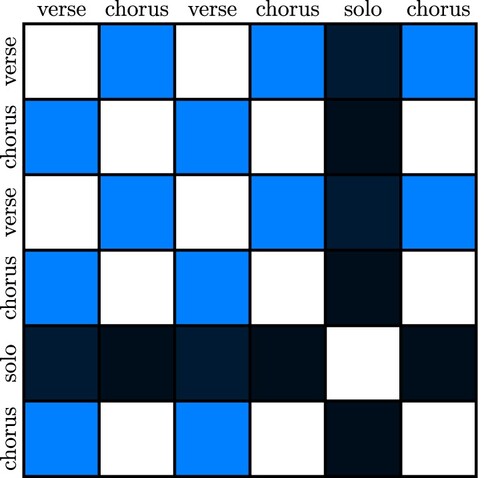
Consider a song whose structure falls into the typical verse-chorus-verse-chorus-solo-chorus progression. If comparing the different sections of the song, one could see that the verses and chorus repeat themselves. Moreover, if possible to quantify the difference between the sections, one could see that the solo is likely to be more different than the verses and the chorus. Representing these observations into a 2-dimensional matrix whose entries correspond to the general similarity between sections, something similar to Figure would be obtained. Now, this representation is not strongly dependent on the song in terms of notes, chords, or tempo, but rather on its general structure, making it a useful tool to compare songs based on their pattern structure.
Figure 1. A possible depiction of a song with the structure verse-chorus-verse-chorus-solo-chorus. White means that the two sections are the same, dark means that they are very different, and a scale of blue is used to interpolate in-between. In most songs, the solo is very different from the rest of the songs, whereas the difference between the verse and the chorus is not as significant. This representation only depends on the structure of the song and not on its notes, tempo, or genre.
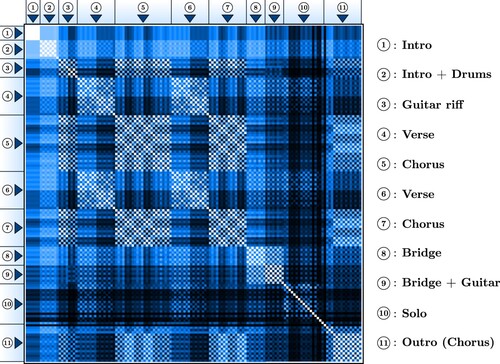
The previous analysis and example use a rather simple approach to divide a song into large sub-sections: verse, chorus, solo, etc. By doing a finer level of analysis, one could hope to highlight these macroscopic behaviours, as well as finer sub-patterns. Overall, the level at which the analysis is done can greatly influence the appearance of the results. In this study, since the representation is obtained from standard musical notation scores, a common subdivision is the bar length. The types of results and figures obtained in this study are summarised in Figure , which transforms the song Beat It by Michael Jackson into a 2-dimensional matrix where each entry describes the similarity between the bars of the song. Observe that the diagonal (top-left to bottom-right) is white since it corresponds to the similarity between the same two bars.
Figure 2. The representation of the song MICHAEL JACKSON – BEAT IT and its structure decomposition. The song can be read in two directions: from left to right or from top to bottom, each square representing the similarity between two bars (see Section 2 for the precise definition of the matrix and Section 3 for its re-normalisation). Lighter squares correspond to smaller entries in the pattern matrix and darker squares correspond to larger entries, making the different sections of the song visible from the variation of shades.
An important property for representing songs into matrices is that it is possible to transform abstract objects (songs) into mathematical objects (matrices), for which standard analysis techniques can be applied. This study uses this observation to define a distance D on songs based on their pattern structure. This distance is meant to express the similarity of patterns between different songs. Using D, it becomes possible to identify groups of songs with similar structures.
Having defined D, this study will next extrapolate the statistical properties of song patterns. In particular, the following questions will be addressed.
Given a song feature, such as year, genre or artist, do there exist specific feature values with a common pattern structure? Given a feature, what are the feature values with the least variability in pattern structures?
Given a group of songs with similar patterns, does there exist a corresponding feature value? Does this group correspond to a specific category of songs?
Finally, this study concludes with an analysis of the ability of D to classify songs based on their features. In particular, we will see that the results obtained in the previous section seem to correspond to specific (yet interesting) cases of song similarities, but that the metric D does not encapsulate further properties of the general feature space of songs and thus provides poor results on classification tasks. This then confirms the goal of this tool and the method developed here: it highlights outliers and extreme behaviours while being, on average, rather uncorrelated with the features of the songs.
1.2. Methodology
This study aims to better understand the pattern structure of popular music, i.e. songs that at any point reached the Billboard Hot 100 chart (CitationBillboard, Citationn.d.). To compute the pattern matrices, all songs were used in the form of Guitar Pro files, which contain a wide range of information on the song, such as key signature, chords, tempo, standard notation scores and tablatures, etc; we provide more details on the transformation of standard music notations into similarity matrices in Section 2 and we refer to the official Guitar Pro website (CitationGuitar Pro, Citationn.d.) as well as the Python library used in this work (CitationAbakumov, Citationn.d.) for more information on the characteristic of the format of files used here. On top of the Guitar Pro file, each song is defined by 6 features:
artist: the artist of the song.
title: the title of the song.
year: the first year the song appeared on the chart.
decade: the decade corresponding to the feature year.
genre: the genre(s) of the song.
type: types of genre, obtained from the feature genre.
The reason for considering the year and decade of first appearance on the chart rather than the actual release date is to focus on the evolution of patterns through popular taste, rather than when the songs were actually written and produced. The last feature, type, corresponds to general genres like ‘rock’, ‘pop’, or ‘hip hop’, as well as genre adjectives, such as ‘experimental’, ‘classical’, or ‘psychedelic’. The full list can be found in Corsini (Citationn.d.) in the file dataset/types.json, while the 10 types corresponding to the most genres can be found in Table ; this table can give an idea of what the values of the feature genre and type look like.
1.3. Dataset
For this article, a new dataset of 4166 songs in their symbolic music scores format along with the 6 previously described features was created. The dataset was collected using the Billboard Hot weekly charts dataset (CitationMiller, Citationn.d.), which includes the first four features. A programme (Corsini, Citationn.d.) went through the songs of this dataset and collected the available Guitar Pro files online (exploring CitationUltimate Guitar, Citationn.d.). The genre feature was computed by searching for the song properties on Wikipedia (CitationWikipedia, Citationn.d.) and the type feature was generated using the genre feature. For more details on how the feature values of type were generated, or about this dataset in general, see Appendix 1 or Corsini (Citationn.d.).
Throughout this process, a lot of automation was used and this dataset may contain noise from any of the following steps:
Errors in the original Billboard Hot dataset.
Wrong song downloaded.
Bad Guitarpro file: fewer instruments, only partial song coverage, not the original version, and mistakes in the writing process.
Mismatched genres.
For each such step, human-based controls were put in place to reduce noise. Among these steps, the one which was the most difficult to control was the third step, related to the direct quality of the files. However, this type of noise should only concern a small portion of songs and will not strongly influence the analysis and the results.
2. The pattern similarity matrix
Let be a song divided into its ordered sequence of b bars:
.Footnote1 The pattern similarity matrix P (or simply pattern matrix) is obtained by defining a distance
on bars, used as the entries of P:
If the song is composed of different instruments, the pattern matrix will be computed by summing the contributions of the different instruments:
where
is the set of instruments of
and
is the kth bar of instrument i.
2.1. Distance of similarity on bars
In order to define , bars need to be transformed. The choice of transformation is to consider them as vectors of size s, where s is the number of time subdivisions in the bar. In other words, a bar
is defined as a sequence
where each element
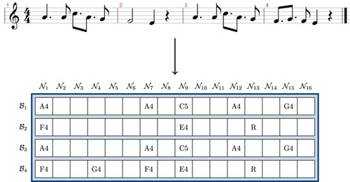
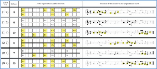
corresponds to the note whose onset is at time t, and s corresponds to the product of the smallest note length (from the whole song) and the ratio of the bar time signature. An example of such representation can be found in Figure , using the main riff of Seven Nation Army by White Stripes.
Figure 3. The representation of the four bars into four vectors of size s = 16. This choice for s follows from the smallest subdivision being a sixteenth note (due to the dotted eighth note) and the bars having a time signature of 4/4, meaning that there is at most
notes in each bar. For each time
, the entry t of the vector corresponds to the onset of the note being played at time t, and is empty otherwise. A special letter,
, is used for a rest.
Let and
be two bars. A definition for
is to count the number of differences between
and
:
where
The reason for this definition of
and δ is that, each time the onset of a note is being played in one of the two bars, it adds one to their distance, except if the same note is being played at the same time in the other bar. From this definition,
, which implies that the range of
is related to the number of notes per bar.
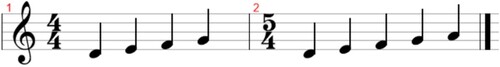
In the definition of , it is assumed that the two bars have the same size s. This does not necessarily follow from the previous definition of s, but can be obtained by normalising the two bars using the smallest note subdivision and the longest time signature ratio. With this definition, if the two bars have different time signatures, then the matrix representation of the bar with a smaller time signature ratio has empty entries past the last time of the bar. This makes every note played at the end of the other bar count as one in the distance
. We provide an example of the computation of
for two bars with different time signatures in Figure .
Figure 4. An example of two bars with different time signatures. If computing for this pair of bars, the result would be 1 since the first four notes are the same and the last note of the second bar corresponds to a time which does not exist in the first bar. This choice comes from the fact that longer bars are usually used to extend a previous pattern (and similarly, shorter bars are usually used to reduce a previous pattern). This choice, however, does not have a significant effect on the results since most of the songs considered here have a classical 4/4 time signatures.
To further illustrate how is computed, we provide in Appendix 2 a few special cases: when the two bars have different time signatures, how rests are dealt with, and how chords are compared to each other. It is worth noting that the definition of
does not depend on s, provided s is large enough to allow
and
to be properly defined (the onset of each note in
and
corresponds to an exact index between 1 and s). Using this remark, when computing the pattern matrix, the same s will actually be used for all bars of the song.
With being defined for any pair of bars, the pattern matrix P of any song can now be computed. As an example, the pattern matrix of the main riff of Seven Nation Army, whose vector representation was given in Figure , can be found in Figure . For the rest of the paper, this exact definition of
is used to compute the pattern matrix of a song. It is worth mentioning however that the images found in Section 4 as well as that of Figure are all re-normalised using ν (defined in Section 3) for clarity.
Figure 5. A representation of the entries of the pattern matrix of the main riff of SEVEN NATION ARMY by WHITE STRIPES. For each row, the first column gives the indices of the two bars being compared, the second column gives the distance between these two bars, the third column gives the two vector representations of the bars obtained in Figure , and the last column gives the original music sheet used to compute the pattern matrix. The notes highlighted in yellow in the third and fourth columns correspond to the differences between the two bars and each yellow square counts as one in the distance of the two bars. From this figure, one can see that the corresponding pattern matrix is given by .
3. Comparing songs
With the pattern matrix of a song defined in Section 2, a distance on pattern matrices can now be computed in order to obtain D, the distance on song structures. This section focuses on the definition of D.
Directly comparing pattern matrices presents a few problems. First of all, they do not necessarily all have the same shape, as P has size , where b is the number of bars of the song. Second, recall that the entries in these matrices are related to the number of notes being played, implying that they can greatly vary between songs. Finally, this link between entries of the pattern matrix and the number of notes played can also create high variability of entries inside a single song, for example, if a sub-section has a much higher density of notes (such as a solo, see Figure ).
For the rest of this section, the goal is to define the function
used to normalise pattern matrices so that they can be easily compared with each other. Here,
is a constant over all songs and
is a normalised pattern matrix and should reflect the pattern structure of P while avoiding the previously raised issues. With ν being defined, the distance over songs D is set as
(1)
(1) where
and
are the pattern matrices of
and
. Here,
is defined as the average
norm; that is, for all A of size
, we have
. The value of p is implied in the definition of D and set to p = 2 for the rest of this study.
It is worth noting that D is actually not a proper metric on the set of songs, but rather a pseudometric: it satisfies all the axioms of a metric except that we might have for two distinct songs
. This property comes from the fact that the pattern matrices of two distinct songs could be the same and that ν is likely not injective (consider the case
for example). The norm
on
however corresponds to a proper metric space.
3.1. Pattern matrix normalisation
Let P be a pattern matrix of size whose entries take values in
. In order to visualise the impact of the different modifications made on P by the normalising function ν, matrices are depicted as in Figure : a white square corresponds to a 0 in the matrix, whereas a black square corresponds to the maximal possible entry, and a scale of blue is used to interpolate values in-between.
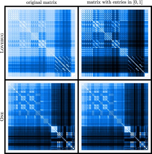
As explained earlier, the entries of P are related to the number of notes being played, which means that these entries can greatly vary between songs. In order to avoid scaling problems when comparing two pattern matrices, their entries have to be taking values in . The importance of this constraint is represented in Figure , where the two songs represented have similar structures but different ranges of entries in their pattern matrices.
Figure 6. Comparison of the songs JONAS BROTHERS – LOVEBUG and METALLICA – ONE before and after normalising their entries between 0 and 1. Each column represents the two pattern matrices on the same scale of blue; the left column corresponds to the original pattern matrices, whereas the right column corresponds to the pattern matrices whose entries have been scaled between 0 and 1. As can be observed from the right column, these two songs have a similar structure. However, if only comparing the values of the two pattern matrices (left column), the entries of the matrix of the METALLICA song are much larger than the entries of the matrix of the JONAS BROTHERS song.
The problem of large entries in pattern matrices does not simply affect comparing two different songs, but can also prevent the matrix of a given song from clearly highlighting its structure. For example, a song with a section denser than the other ones will have very high entries in specific rows and columns of its pattern matrix, making the rest of the entries small in comparison; and this could hide possible sub-patterns of the song. To avoid this issue, the variation of the entries in P is normalised by using the corresponding percentile index rather than the exact value.Footnote2
Write for the sequence of ordered entries of P; in other words,
for
, and
. Let
be the α quantile of
and
be the jth percentile of
. The percentile normalisation function
is defined as
and replaces the entries of P by their corresponding percentile index. An example of the importance of applying
can be found in Figure .
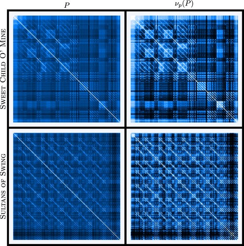
Figure 7. Comparison of the songs GUNS N' ROSES – SWEET CHILD O' MINE and DIRE STRAITS – SULTANS OF SWING with and without applying to their pattern matrices. The left column corresponds to the original pattern matrix and the right column corresponds to its image through
. As can be observed from the left column, a few bars with high distance to the rest of the song tend to make the overall picture uniformly blue, making both of these pattern matrices look similar. However, after applying
, different patterns appear more clearly, showing the diversity in structure of these two songs. This figure also represents the importance of
when representing patterns of songs, since it highlights their patterns.
After applying to a pattern matrix P, the maximal entry is always 100, corresponding to the maximal entries of P. However, the minimal entry might not be 0, for example if there are many 0 in P. In order to avoid this issue, a second normalising function
is applied, forcing the entries of the matrix to take values in
, with 0 and 1 included. More precisely
is defined as
where
. Here,
is used instead of P to highlight the fact that
is supposed to be applied to the image of P through
and not directly to the pattern matrix P. The effect of
on
is depicted in Figure . The changes operated by
are not meant to have a strong impact on the whole process, but give a desired property for the resulting matrix: bars which are the same correspond to entries with value 0, and bars with most differences correspond to entries with value 1.
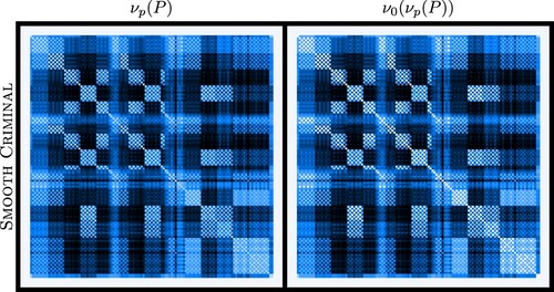
Figure 8. Comparison of and
for the pattern matrix P of the song MICHAEL JACKSON – SMOOTH CRIMINAL. The main difference between these two pictures is that the lightest colour on the left image is not exactly white, meaning that the smallest entries of the matrix are not exactly 0. Even though
does not greatly modify the matrix, the patterns appear slightly clearer on the right.
When applying and then
to a pattern matrix P, it is transformed into a matrix of size
whose entries take values in
. Moreover, the resulting matrix clearly represents the structure of the original song, meaning that it can be used to compare the structure of different songs. Before being completely able to compare songs according to their pattern matrices, it remains to address the variety in sizes b of the matrices. Since b corresponds to the number of bars of the song, it is most likely different from one song to the other.
3.2. Resizing matrices
Consider two normalised pattern matrices and
of respective sizes
and
, obtained as the image of two pattern matrices through
. A straightforward way to compare
and
in spite of their respective sizes is to extend them by repeating each of their entry multiple times. More precisely,
and
are transformed using σ, defined as follows
The image of
through σ is a pair of matrices, whose sizes are both
, and whose entries are related to the entries of
and
repeated multiple times:
times for the entries of
and
for the entries of
. Using σ, let the true distance
of
and
be defined by
where
. Note that this distance also corresponds to a graphon-like approach (Lovász & Szegedy, Citation2006). Indeed, if
and
are transformed into functions
such that
and
, then
is equal to their integral
distance
(2)
(2) This approach reinforces the idea that this should be the true distance between pattern matrices.
The function , although perfectly adapted to compute the distance between normalised pattern matrices, is not computationally feasible since it requires to use matrices of size
; even if replacing bd by the lowest common multiple of b and d, the computation time is unrealistic (see the first column of Table ). To avoid this computational problem, an approximation of
is used.
Table 1. Comparison of with
for
.
Fix an integer and let
be defined as follows
This function, similar to σ, creates a matrix of size
whose entries are related to the entries of
. However, since
might not be a multiple of b, the number of times each entry of
is repeated in
is not necessarily constant, creating a small error in the representation of
. Define now
by
Since
slightly modifies the role of the entries of the matrix
, the distance
is not necessarily going to be equal to
. However, for any pair of matrices
and
, the distance
converges to
as
increases to infinity; if considering the integral definition of
as in (Equation2
(2)
(2) ),
actually corresponds to the Riemann approximation of
using squares of size
.
Computing requires using matrices of size
. This means that the smaller
is, the faster the computation will be. Hence, it is interesting to choose a value for
that balances between the computational time of
and the accuracy compared to the true distance
. Table gives an approximation of the computational time and the accuracy for different values of
. From this table, any
larger than 100 is an appropriate choice since the error rate is less than
. For the rest of this study,
is set to be 500, corresponding to an error rate as small as computation time reasonably allows.
To conclude this section, ν is set to be the combination of the different normalisation functions:
In other words, the image of a pattern matrix P through ν corresponds to transforming P using its percentiles (see Figure ), then forcing its values to span 0 and 1 (see Figure ), and finally resizing it to
. Using the image of ν as a normalised pattern matrix, the pattern structure of songs can be compared by defining the similarity distance on songs D as in (Equation1
(1)
(1) ).
4. Results
With the pattern matrix being defined in Section 2 and the distance D set in Section 3, songs can now be compared according to their pattern structures. In this section, the values given by D are combined with the features of the songs (defined in Section 1.2) to answer the previously asked questions:
Given specific feature values, what can we say about the pattern structures?
Given similar pattern structures, do they have corresponding feature values?
To answer these questions, two scores are defined on groups of songs: the pattern variability score ( score) and the feature variability score (
score).
Let be a group of songs. The
score of
is defined as the average distance between any pair of songs of
:
This score should be interpreted as the amount of variability between the patterns of the songs of this group: groups with a small
score correspond to a set of songs whose patterns are similar.Footnote3
Given this same group of songs , let
be their feature values, corresponding to the feature F taken from the possible choices of features: artist, title, year, decade, genre, or type. The
score of
(with regards to F) is defined in one of the following two ways. If
are real numbers (meaning that
), then the
score is the standard deviation of the values
:
where
. Otherwise, if
are not real numbers, then the
score is defined as the average of the counting process of
. More precisely, let
be such that
,
and
. Then, the
score is defined as
This choice of score can be seen as transforming
into a set of probabilities
, where ℓ is the number of different feature values in
and
is the probability of having the jth most common feature value when sampling a random
. With this approach,
then corresponds to the average popularity of the chosen index. For example, imagine having a group of 10 songs, and consider the three following cases along with their
scores.
All songs have the same feature value; in that case
and
The songs take two possible feature values, separated into two groups of equal sizes; in that case
All songs have different feature values; in that case
In both cases whether are real numbers or not, the
score should be interpreted as the amount of variability between the feature values of the songs of this group: groups with a small
score correspond to a set of songs with a lot of similar features.
With the and the
scores defined, the rest of this section is organised as follows. Section 4.1 uses a feature-based approach and studies the
score when grouping songs according to their feature values. For each feature, this allows a ranking of the feature values according to their variability of patterns. Sections 4.2 and 4.3 create groups of songs according to the distance D and study the
score of these groups. Section 4.2 uses a cluster-based approach and partitions songs into clusters, whereas Section 4.3 uses a neighbour-based approach and focuses on each song's nearest neighbours. These two approaches give similar results and are both efficient in finding underlying properties of features not observable with the approach of Section 4.1. Finally, some extra figures completing those presented in the following sections can be found in Appendix 3
4.1. Pattern variability on features (feature-based approach)
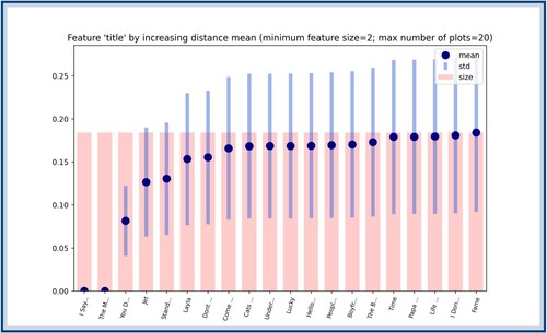
Consider the different features of a song: artist, title, year, decade, genre and type. Each of these features has a set of possible values it can take; for example, all songs of the dataset in this study appeared in the chart for the first time between 1958 and 2019. Now, for each feature value, all corresponding songs can be grouped together and their score can be computed. For example, the first 20 lowest
scores for the feature year are represented in Figure .
Figure 9. The year 1958 to 2019 ordered according to their score (only the first 20 lowest ones are depicted here). The blue dots correspond to the
scores, which are obtained by computing the average distance between songs from a given year. The blue bars show the standard deviation around this average distance. The bars in red represent the number of songs who appeared for the first time the corresponding year. No year has a notably lower score than the next one, but this computation gives a ranking on years according to their variability in pattern structure.
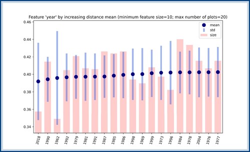
Figure 10. The artists with lowest score according to different threshold on their minimal number of songs. On the left, three figures correspond to the first 20 scores for the feature artist, where the minimal number of songs is set to 2, 5 and 10. On the right, all the normalised pattern matrices of each artist with lowest score. As the number of songs for each feature value increases, so does the variety of patterns, making it more difficult to explain the low score with the pattern matrices.
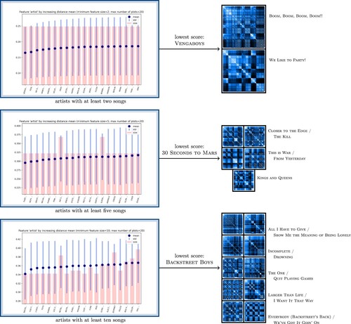
The score of each feature value is a clear and easy-to-interpret metric. However, this score is difficult to combine with the actual pattern matrices, since it reflects a general trend rather than the existence of a unique pattern structure. Indeed, when the number of songs for each feature value is large, then the number of pattern structures tends to be large as well. Figure illustrates this principle by representing the artists with at least 2, 5 and 10 songs and with minimal
score. From this figure, one can see that, as the number of songs considered increases, the number of pattern structures also increases.
A possible explanation for the limited interpretation of , is that it only focuses on the average distance between a given group of songs
. As explained, this means that, as the size of the group increases, the average distance will converge to a standardised distance. Even without a group of large size, issues of interpretation can appear. For example, it is possible for
to be composed of songs having one of two distinct pattern structures; in this case, even though the pattern variability of
would be limited, since patterns of songs in
could be explained by only two types of pictures, the
score of
would be high, because the average distance would be related to the distance between the two distinct patterns. In order to avoid such issues, Sections 4.2 and 4.3 focus on studying the variability in features from groups of songs with similar patterns, rather than considering all songs with the same feature value. These two sections give a better understanding of the structural properties of songs and their relation to features.
The score is limited in its interpretation and might miss interesting underlying properties of the relation between features and patterns. However, this score is a natural approach to studying pattern variability in songs and it gives a metric allowing the direct ranking of feature values. It might require some modification and improvement (see Section 6 for further ideas), but could be used as an interesting metric to study the evolution of variability through years, genres, or artists (see Appendix 3 for the complete set of figures regarding the
score).
4.2. Feature variability on clusters (cluster-based approach)
After considering each feature independently and giving a score for each feature value according to pattern variability, this section applies first the distance on song D to create clusters. Once these clusters are identified, their score is computed, highlighting clusters with repeating feature values.
Since clusters can greatly vary according to the method used, three common clustering algorithms were implemented:
Spectral Clustering (Ng et al., Citation2001);
K-Medians (Park & Jun, Citation2009); and
Agglomerative Clustering (Ward Jr, Citation1963).
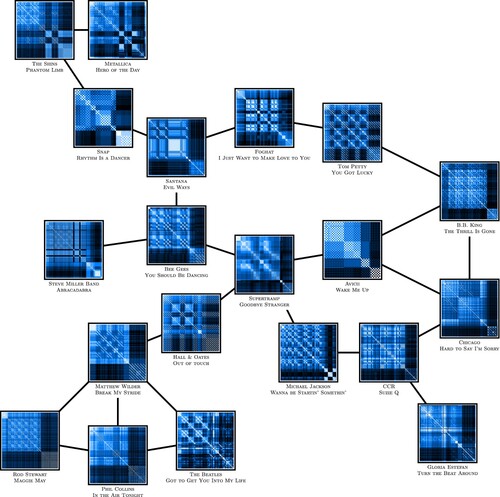
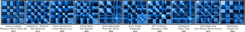
The choice of algorithms was motivated by two constraints. First, these algorithms can be directly applied to a pre-computed distance matrix obtained from D, and do not need to access the embedding space of the songs; this first reason explains why K-Medians was chosen over the more classical K-Means. Second, the number of output clusters is determined by a number given as input; this second reason explains why the classical DBSCAN algorithm is not used here. With these two constraints, Spectral Clustering and K-Medians are standard algorithms. The reason for using Agglomerative Clustering is that it fits the songs into a tree-like structure, which is a good way to interpret song patterns (see Figure ). For this last reason, Agglomerative Clustering gives the best results and all further analysis in this section was obtained using this algorithm (see Appendix 3 for some results on Spectral Clustering and K-Medians).
Figure 11. A representation of the tree-like structure of song patterns. This graph was obtained by connecting songs with their nearest neighbours. From this figure, one can observe that all of the above songs fall into the category of songs with a high outro, represented by darker bands at the bottom and at the right of the figures. From this general pattern structure category, sub-types of patterns can be observed and the connections between these patterns create a tree-like structure.
Since the dataset contains a large number of songs (4166 in total, see Appendix 1), and the size of the clusters should be limited for interpretative reasons, a recursive approach was used. The actual clustering algorithm is described in Algorithm 1 and is based on applying one of Agglomerative Clustering, Spectral Clustering, or K-Medians recursively, to reduce the clusters to a desirable size. The results that follow are all obtained by using Agglomerative Clustering (with output clusters), no limit on the maximal number of iterations (
), and clusters of size at most 15 (
).
Once Algorithm 1 is applied to the set of songs, a similar approach to Section 4.1 is used and clusters are ranked according to their score. A typical outcome of this algorithm can be found in Figure , where clusters are ordered according to their
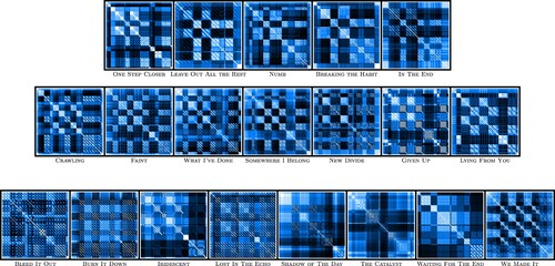
score with regards to the feature year. Once this figure is obtained, it needs to be combined with an analysis of the clusters; the cluster with the lowest score in Figure is represented in Figure .
Figure 12. Clusters ordered according to their score with regards to the feature year (only depicting the 20 lowest scores). The blue dots represent the average year of the cluster, the blue bars represent the standard deviation around this year and the red bars represent the sizes of the clusters. This figure needs to be combined with a representation of the clusters in order to appreciate its results. The cluster with the lowest score is represented in Figure .
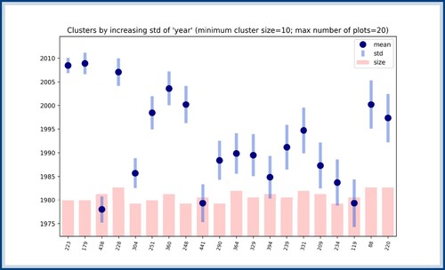
Figure 13. A representation of the cluster with lowest score as found in Figure . As one can see, all songs show a similar pattern and have been released around the same years. Since this cluster was obtained by grouping songs according to their pattern similarities, it also means that this specific pattern is characteristic of the end of the 2000's.
Our interest in using clusters instead of the feature-based approach of Section 4.1 can be understood by considering the results of Figure . Indeed, the feature-based approach considers every feature value independently of each other and then ranks them according to their score. However, in the case of the feature year, for example, feature values can be compared with each other and a notion of proximity can be defined. Using this property, the cluster represented in Figure can be found, where the pattern clearly corresponds to songs around the year 2010. This could not have been unveiled by the feature-based approach in Section 4.1 since it does not compare songs that have different but similar feature values.
The reason for using the cluster-based approach over the feature-based approach is not limited to the notion of proximity on the feature year. As explained in Section 4.1, a possible limitation of the score is that it is not able to detect groups of songs that would be generated from a couple of distinct pattern structures. Clustering methods, however, are able to separate songs according to pattern similarity and then identify groups with repeated feature values. An example of the power of clusters in identifying sub-groups of patterns inside a given feature value is represented in Figure , where the artist Linkin Park shows two commonly used structures. The reason this artist did not appear clearly in the results of Figure is due to the two limitations of the
score explained in Section 4.1: this artist has a lot of songs and a combination of different but repeated pattern structures.
Figure 14. A representation of all the pattern matrices of the artist LINKIN PARK. The top two groups each correspond to a specific type of pattern and the bottom group contains the rest of the songs. This grouping shows that the artist LINKIN PARK commonly uses one of the two top structures. This property is highlighted by clusters but was missed when considering the score on the artist as shown in Figure . Two reasons can explain why this artist does not have a low
score: the large number of songs it has in the dataset, and the fact that they mostly correspond to one of two distinct pattern structures.
Using the score on clusters shows more promising results than using the
score on songs grouped by their feature values, since it is able to highlight finer properties of song patterns. One reason for this improvement is that the cluster-based approach is able to ignore noisy or out of distribution songs and only focuses on groups with similar structures. This leads to a better ability to identify specific pattern structures related to years (Figure ) or artists (Figure ). A few figures showing what happens when considering the features genre and type can be found in Appendix 3.
4.3. Feature variability on neighbourhoods (neighbour-based approach)
The cluster-based approach used in Section 4.2 is useful since it creates a partition of the songs into groups. This approach also implies that groups with low scores can be interpreted as patterns characteristic of the given feature value (as explained in Figure ). However, another possible approach to grouping songs is to consider the set of nearest neighbours for each song.
For each song in the dataset, using the distance D it is possible to identify its neighbourhood, hence creating groups of songs with a centre. With this approach, some songs might appear in more neighbourhoods than others. This remark implies that neighbourhoods cannot be interpreted as characteristic groups, as was the case with clusters; however, this technique allows the definition of a centre song, opening more possibilities with the analysis of features.
Consider computing the 20 nearest neighbours of all the songs. For each of these neighbourhoods, the corresponding score can be computed as in Section 4.2. Furthermore, since neighbourhoods have a centre song, it is now possible to compare the feature of the centre with its neighbours. By applying this idea to the neighbourhoods ordered according to their
score with regards to the feature year, Figure is obtained and compares the neighbours and the centre song years of first appearance in the chart.
Figure 15. Neighbourhoods ordered according to their score with regards to the feature year. The blue dots, blue bars, and red bars respectively represent the average year, the deviation around this average year, and the average distance between songs of the neighbourhoods. The yellow star represents the year of the centre song. This approach allows the identification of songs with early use of patterns (such as the first song, HEART – IF LOOKS COULD KILL), late use of patterns (such as the second song, SIA – THE GREATEST), or on-time use of patterns (such as the third song, JOJO – LEAVE (GET OUT)). A few neighbours of HEART – IF LOOKS COULD KILL are represented in Figure .
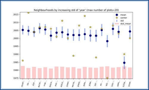
Figure 16. The representation of the song HEART – IF LOOKS COULD KILL, as well as a few chosen neighbours. As it appears from this figure, the pattern shown by HEART – IF LOOKS COULD KILL is borrowed by songs released years later. Moreover, it is interesting to notice that the songs represented below all fall under some genre related to rock and could thus be interpreted as a revival of the original hard rock structure found in the HEART song.
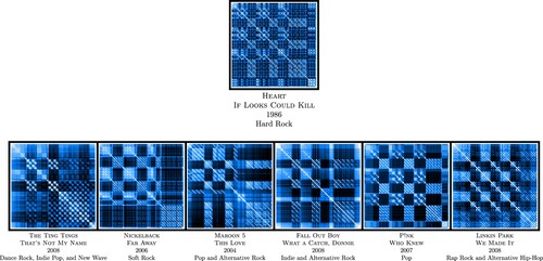
An interesting analysis of the feature year, made possible by neighbourhoods, can be done by classifying song patterns as early, late or on-time (see Figure ). By considering neighbourhoods with the lowest with regards to the feature year, meaning neighbourhoods with the lowest year standard deviation, and comparing the average year of the neighbourhood to the year of the centre song, three behaviours can be identified. Songs can either have pattern structures similar to songs appearing later in the chart, meaning that this pattern was ahead of its time. Similarly, songs can have pattern structures that were commonly used in earlier years, meaning that they could have been inspired by previously released songs. Finally, songs can have pattern structures similar to other songs of the same year. In this last case, it is possible that the cluster-based approach of Section 4.2 would have already identified this relation between pattern and years, whereas the first two cases would tend to be hidden when studying the
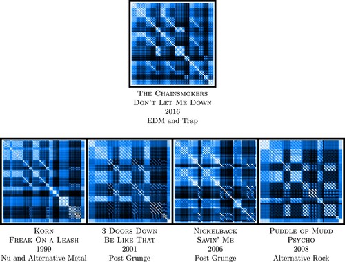
score of the clusters. Two interesting examples of a song with early and late pattern structures can be found in Figures and , where both the features year and genre have interesting behaviours. Indeed, in the case of Figure , the pattern is later borrowed by the neighbours of the Heart song and can be interpreted as a revival of the original song style, whereas in the case of Figure , the strong difference in both years and genre shows the originality of the structure of the The Chainsmokers song.
Figure 17. The representation of the song THE CHAINSMOKERS – DON'T LET ME DOWN, as well as a few chosen neighbours. As it appears from this figure, the pattern shown by THE CHAINSMOKERS - DON'T LET ME DOWN is taken from an early period. Moreover, when comparing the genre of these different songs, it also appears as THE CHAINSMOKERS – DON'T LET ME DOWN does not fit the genres of its neighbours. This is an interesting example of song whose patterns is borrowed from another period of time and style of music.
Overall, the cluster-based approach of Section 4.2 and the neighbour-based approach of this section give similar and complementary results. While the cluster-based approach highlights characteristic patterns corresponding to feature values, the neighbourhood approach can be used to find outliers in pattern structures by showing songs whose features are unrelated to those of their neighbours. These two techniques can also be combined to help understand the general structure of the song patterns. Indeed, by comparing clusters and neighbourhoods, one can observe a possible tree-like structure for song patterns, as highlighted in Figure . This might also explain why the Agglomerative Clustering algorithm shows better results than the two other clustering techniques considered.
5. Evaluation
In order to complete this study, we evaluate the ability of the metric D to classify songs. More precisely, we implement various classical regression and classification algorithms to test whether D can be used to predict the features year, decade, artist, genre, and type.
The problem we are trying to solve can be formally stated as follows. First of all, we have a set of songs which we divide into two sets:
for the train set and
for the test set. In our case, we randomly split
so that
, meaning that the train set is
of the dataset and the test set corresponds to the remaining
. Second, we have a distance D defined on
and, for each song
, we have a feature
(we later explain how the different formats of features are handled). Our goal is to define a classification function
which is constructed using
and so that
The meaning of the ≃ will be later clarified, but should be understood as φ correctly classifies
as having the feature
. We now describe the different algorithms considered to define φ.
All of the regression and classification algorithms considered here come from the scikit-learn (Pedregosa et al., Citation2011) library in Python. In particular, we use the following algorithms.
LinearRegression (LR), from the linear_model module, computing a simple linear regression;
KNeighborsRegressor (KNR) and KNeighborsClassifier (KNC), from the neighbors module, computing a nearest neighbour regression and classification;
SVR (SVR) and SVC (SVC), from the svm module, computing a support vector regression and classification;
GaussianNB (GNB) and BernoulliNB (BNB), from the naive_bayes module, computing two types of naive Bayes' estimations; and
DecisionTreeRegressor (DTR) and DecisionTreeClassifier (DTC), from the tree module, computing a decision tree regression and classification.
We further test two versions of the nearest neighbour regression and classification, using either 10 neighbours (10NR and 10NC) or 20 neighbours (20NR and 20NC). The other parameters of the models were unchanged from their defaults features.
Note that only four of the aforementioned algorithms allow the input to be a pre-computed distance: SVR, SVC, KNR, and KNC. For the other five, we decided to emulate a vector space by splitting the train set using a basis of songs. Let
be a random subset of the training set. Then, we embed the remaining set of songs
along with the distance D as a vector space of dimension
by saying that the coordinates of
are given by
. This thus allows us to apply the remaining algorithms, LR, GNB, BNB, DTR, and DTC, to this vector space. For the rest of this study, we set
so that it corresponds to approximately
of the songs of the train set, chosen at random.Footnote4
Since we want to test different formats for the features, numerical for year and decade, categorical for artist, and multi-categorical for genre and type, we need to set up different evaluation methods. In the case of numerical values, that is when and φ both output numbers, we implement the two metrics
for the average error in classification, and
where
if and only if x = 0, for the number of successes. It is worth noting that a good classification algorithm should output a low
and a high
(in percentage). Running the previous algorithms on our dataset leads to Table .
Table 2. The classification results for the two numerical features, year and decade.
As we can see in Table , the results show that D is not a good metric for characterising the year or decade of a song. Indeed, on average it misclassifies the song by at least 10 years and does not classify songs substantially better than a simple random classification. We now provide the results for categorical feature values, that is for the feature artist. In this case, regression algorithms cannot be applied and the score defined before is not properly defined anymore. However, the SUCC score still makes sense in this context and we thus provide the results of the classification algorithm on the feature artist in Table .
Table 3. The classification results for the categorical feature artist with respect to the SUCC score.
As we expected given the observations from Section 4.1, and in particular the observations made in Figure , the metric D does not properly encapsulate the properties of the artists to characterise them. Furthermore, in the case of the artist features, since it is very diverse (1431 different feature values out of the 4166 entries of the dataset), one cannot expect the training set to cover enough information for the algorithm to be able to properly classify songs of the test set. For this feature, we are actually in the case of the curse of dimensionality and would likely need to greatly increase the size of the dataset while keeping the same number of artists to have a chance to solve this problem. We now conclude this section with the evaluation strategy for multi-categorical feature values.
Recall that, in the case of the features genre and type, and φ are both lists of categorical values. To represent this, we identify
and the output of φ with a distribution on
, where
is the set of feature values (for example ‘alternative rock’, ‘brit pop’, and ‘gangsta rap’ for genre and ‘rock’, ‘alternative’, and ‘art’ for type). More precisely,
is defined by
In particular, this implies that
A similar definition is used for
. In other words, we see
and
as measures of probability on
corresponding to the odds of
to take a specific feature value. We now consider the following evaluation metrics for multi-categorical features. Write
for the function such that
if and only if x>0.
The correctness, corresponding to the fact that any one of the guessed feature in φ is correct:
The precision, corresponding to the ratio of correctly guessed features of
The accuracy, corresponding to the probability of correctly guessing a feature of
The exact matching, corresponding to the number of features exactly evaluated by φ:
To understand better these metrics, let us consider a couple of specific cases.
Imagine that φ always guesses that each song has all possible feature values:
Imagine that φ always guesses a single and correct feature:
With that in mind, a high or
score should be evaluated with the corresponding
and
scores: if the latter ones are low this only means that the classification function gives a lot of features for each song. The evaluation of
with regards to these different metrics on genre and type can be found in Table .
Table 4. The classification results for the two multi-categorical features, genre and type.
Observing the results from Tables , it is clear that D does not provide good results in terms of classification. Indeed, in all the considered cases, the results do not substantially improve a simple random guess. However, this should not fully come as a surprise: D was designed to extract anomalous behaviours from a song dataset and did not intend to provide global properties.
The low classification scores of D can actually be related to the results from Section 4.1. Indeed, we observed there that D did not provide clear rankings of the features and explained that, when considering many songs, the pattern matrices would cover a wide range of behaviours and would thus cancel the effect of D. Thus, in order for D to show its true potential, one need to more precisely analyse relations between smaller groups; we were able to so in Sections 4.2 and 4.3, where we found interesting and surprising relations between specific features and patterns. It is then not surprising that these specific and outlying behaviours do not show in the results of Tables .
6. Discussion
Embedding songs into 2-dimensional similarity matrices is a powerful tool for modelling their underlying structure. Moreover, this embedding can be applied to compare songs with each other according to their pattern structures. This approach allows the definition of precise metrics on groups of songs which helps to unveil underlying commonalities amongst artists, years, or genres. By defining the similarity matrices and the distance on these matrices, one can observe interesting repetitions and commonly used structures over a large set of songs.
6.1. Outcome of present study
A common approach to group songs is according to some known information, such as by artist, or year, before comparing their pattern structures. This leads to the definition of the score and the study of Section 4.1. Although theoretically interesting, this method shows limitations due to the inevitable variety of structures which appear when comparing multiple songs (see the analysis made in Figure ). To minimise such problems, two possible improvements on the
score could be implemented.
The first improvement would be to normalise all groups to the same size. This could be done either by changing the dataset directly or by computing differently the score: for example, instead of summing the average distance over all songs, just consider the N closest songs, with N being fixed over all groups. If N is well-chosen, this could balance the bias towards small groups, observed in Figure , by making large groups more likely to have a small
score. However, this would tend to ignore sub-groups of songs, making this analysis less objective.
The second improvement would be to combine these groups with a clustering algorithm in order to reduce the noise created by outliers. In that sense, this method would be more similar to the cluster-based approach of Section 4.2, but where all the clusters must have the same feature values, and would thus likely only provide small improvements.
The limitation of the feature-based approach, that is sorting features according to their score, pushed for further studies on the relation between D and the song features. This led to the cluster-based approach of Section 4.2 and the neighbour-based approach of Section 4.3. By first using D to create relevant groups of songs and then computing their
score, it is possible to highlight inherent properties that were not observable when simply grouping songs according to their feature values (see Figures and ). Both of these two grouping methods showed similar results as they were able to find groups of songs with repeating feature values that were previously missed. These two methods also complete each other. Since the cluster-based approach creates a partition of the songs, each group can be defined as the representation of a specific pattern structure. Hence, by finding groups with similar feature values, these groups can be interpreted as a typical structure used for this feature value and not elsewhere. Conversely, the neighbour-based approach tends to put some songs into more neighbourhoods than others and cannot be interpreted as typical for the structures. However, it allows the comparison of a song with other similar ones and is able to identify songs with unexpected patterns (see Figures and ).
6.2. Possible follow-up analysis
While the novelty of this study was mainly based on comparing similarity matrices of songs, the full use of the information available in standard symbolic music notation could open the door to further development in music analysis. First, new types of similarity matrices could be defined. For example, if instead of comparing the notes played between bars, the representation was using the position of the notes in the current chord, then the similarity matrices could contain some finer information on the evolution of the song. In this case, a simple pattern being repeated on different scales could be discovered, and this could lead to a better definition of pattern matrices. Second, the full use of standard music notation could also be useful when comparing different songs. Either by directly comparing what is being played or by comparing chord progressions, a new distance on songs D could be defined, not directly related to the pattern structure but rather to the composition structure. Finally, by only considering a subset of the instruments of the song, this method could be used to characterise songs according to specific metrics (for example the drum patterns, or the rhythmic patterns). Using this approach could also lead to representing songs with multiple similarity matrices, according to the different instruments, and then using more complex statistical tools to study their properties.
This study opens the door to further development in music structure analysis, especially in the field of similarity matrix representation. With our newly created dataset, made of standard music notations of songs, new types of similarity matrices can be defined, for example by borrowing methods from music theory. The novel approach of this study, based on comparing similarity matrices rather than analysing them individually, also creates new tools for the analysis of song structure. It is now possible to classify a large number of songs by similarity of patterns and to highlight repeated structures used by artists, years, or genres.
Finally, the grouping methods applied above were able to extract certain groups of songs with interesting behaviour. The outcome of this project could thus be combined with a finer analysis of the properties of some of these songs. For example, one could study in more details the full discography of the artist LINKIN PARK, as it appears to often use similar structures (see Figure ), or compare other properties of the songs from Figures and , such as their chord progression or the structure of the different instruments.
Acknowledgement
This project all started from a discussion with J. Barrett on basic drum beats, where his input made me question the structure of popular songs. I also wish to thank Dr. Addario-Berry for his support on this project, as well as his two colleagues, Dr. Ouzounian and Dr. Hasegawa, for their input in creating the background of this study. I am also very grateful to N. Kauf, T. Voirand, and T. Stokes for proofreading this work and for their advice. Finally, I would like to thank two anonymous referees whose inputs greatly improved the quality of this paper.
Disclosure statement
No potential conflict of interest was reported by the author(s).
Additional information
Funding
Notes
1 It is worth noting that the bar decomposition is not unique; for example, one bar of 4/4 can also be seen as two bars of 2/4. This could be a problem if the file is poorly written and/or if the songs are composed of complex metres, but is mostly irrelevant in the case of popular music, usually encoded by a standard 4/4 time signature.
2 The reason for choosing the percentile index instead of a more common activation function, such as softmax or softmin, comes from the desire to completely remove the bias created by large entries in the matrix, instead of just reducing it.
3 An easy way to better understand the score is by comparing the results of Figure with that of Figure ; indeed, the lowest scores in Figure all correspond to covers of the same song and are thus lower than the lowest scores in Figure .
4 Some extra experiments were implemented using different percentages of the train set for the basis set but mostly provided similar results and we thus decided not to include them for clarity.
References
- Abakumov, S. (n.d.). PyGuitarPro. https://github.com/Perlence/PyGuitarPro.
- Bartsch, M. A., & Wakefield, G. H. (2001). To catch a chorus: Using chroma-based representations for audio thumbnailing. In Proceedings of the 2001 IEEE Workshop on the Applications of Signal Processing to Audio and Acoustics (Cat. No. 01TH8575) (pp. 15–18). IEEE.
- Bartsch, M. A., & Wakefield, G. H. (2005). Audio thumbnailing of popular music using chroma-based representations. IEEE Transactions on Multimedia, 7(1), 96–104. https://doi.org/10.1109/TMM.2004.840597
- Billboard (n.d.). Billboard Hot 100. https://www.billboard.com/charts/hot-100.
- Buisson, M., Mcfee, B., Essid, S., & Crayencour, H. C. (2022). Learning multi-level representations for hierarchical music structure analysis. In International Society for Music Information Retrieval (ISMIR). (pp 591–597).
- Cambouropoulos, E., & Widmer, G. (2000). Automated motivic analysis via melodic clustering. Journal of New Music Research, 29(4), 303–317. https://doi.org/10.1080/09298210008565464
- Cope, D. (2009). Hidden structure: Music analysis using computers. AR Editions, Inc.
- Corsini, B. (n.d.). Gituhub repository.music-patterns, https://github.com/BenoitCorsini/music-patterns
- de Clercq, T. (2012). Sections and successions in successful songs: A prototype approach to form in rock music. University of Rochester.
- de Clercq, T. (2017). Interactions between harmony and form in a corpus of rock music. Journal of Music Theory, 61(2), 143–170. https://doi.org/10.1215/00222909-4149525
- Eerola, T., Järvinen, T., Louhivuori, J., & Toiviainen, P. (2001). Statistical features and perceived similarity of folk melodies. Music Perception, 18(3), 275–296. https://doi.org/10.1525/mp.2001.18.3.275
- Epstein, P. (1986). Pattern structure and process in Steve Reich's ‘Piano Phase’. The Musical Quarterly, 72(4), 494–502. https://doi.org/10.1093/mq/LXXII.4.494
- Foote, J. (1999). Visualizing music and audio using self-similarity. In Proceedings of the Seventh ACM International Conference on Multimedia (Part 1) (pp. 77–80). ACM digital library.
- Foote, J. (2000). Automatic audio segmentation using a measure of audio novelty. In 2000 IEEE International Conference on Multimedia and Expo. ICME2000. Proceedings. Latest Advances in the Fast Changing World of Multimedia (Cat. No. 00TH8532) (Vol. 1, pp. 452–455). IEEE.
- Foote, J., & Uchihashi, S. (2001). The beat spectrum: A new approach to rhythm analysis. In IEEE International Conference on Multimedia and Expo, 2001. ICME 2001 (pp. 224–224). IEEE Computer Society.
- Guitar Pro (n.d.). Software. https://www.guitar-pro.com/.
- Harkleroad, L. (2006). The math behind the music. Cambridge University Press.
- Jiang, J., Chin, D., Zhang, Y., & Xia, G. (2022). Learning hierarchical metrical structure beyond measures. In ISMIR 2022 Hybrid Conference. (pp. 201–209).
- Lovász, L., & Szegedy, B. (2006). Limits of dense graph sequences. Journal of Combinatorial Theory, Series B, 96(6), 933–957. https://doi.org/10.1016/j.jctb.2006.05.002
- Miller, S. (n.d.). Billboard hot weekly charts. https://data.world/kcmillersean/billboard-hot-100-1958-2017.
- Ng, A., Jordan, M., & Weiss, Y. (2001). On spectral clustering: Analysis and an algorithm. Advances in Neural Information Processing Systems, 14, 849–856.
- Nieto, O., Mysore, G. J., Wang, C.-i., Smith, J. B., Schlüter, J., Grill, T., & McFee, B. (2020). Audio-based music structure analysis: Current trends, open challenges, and applications. Transactions of the International Society for Music Information Retrieval, 3(1), 246–263. https://doi.org/10.5334/tismir.78
- Osborn, B. (2013). Subverting the verse–chorus paradigm: Terminally climactic forms in recent rock music. Music Theory Spectrum, 35(1), 23–47. https://doi.org/10.1525/mts.2013.35.1.23
- Park, H.-S., & Jun, C.-H. (2009). A simple and fast algorithm for k-medoids clustering. Expert Systems with Applications, 36(2), 3336–3341. https://doi.org/10.1016/j.eswa.2008.01.039
- Paulus, J., & Klapuri, A. (2006). Music structure analysis by finding repeated parts. In Proceedings of the 1st ACM Workshop on Audio and Music Computing Multimedia (pp. 59–68). ACM Digital Library.
- Paulus, J., & Klapuri, A. (2009). Music structure analysis using a probabilistic fitness measure and a greedy search algorithm. IEEE Transactions on Audio, Speech, and Language Processing, 17(6), 1159–1170. https://doi.org/10.1109/TASL.2009.2020533
- Pedregosa, F., Varoquaux, G., Gramfort, A., Michel, V., Thirion, B., Grisel, O., Blondel, M., Prettenhofer, P., Weiss, R., Dubourg, V., Vanderplas, J., Passos, A., Cournapeau, D., Brucher, M., Perrot, M., & Duchesnay, E. (2011). Scikit-learn: Machine learning in python. Journal of Machine Learning Research, 12, 2825–2830.
- Pienimäki, A., & Lemström, K. (2004). Clustering symbolic music using paradigmatic and surface level analyses. In Proceedings 5th International Conference on Music Information Retrieval.
- Rafii, Z., & Pardo, B. (2011). A simple music/voice separation method based on the extraction of the repeating musical structure. In 2011 IEEE International Conference on Acoustics, Speech and Signal Processing (ICASSP) (pp. 221–224). IEEE.
- Rafii, Z., & Pardo, B. (2012). Music/voice separation using the similarity matrix. In ISMIR (pp. 583–588).
- Salamon, J., Nieto, O., & Bryan, N. J. (2021). Deep embeddings and section fusion improve music segmentation. In ISMIR (pp. 594–601).
- Silva, D. F., Yeh, C. -C. M., Zhu, Y., Batista, G. E., & Keogh, E. (2018). Fast similarity matrix profile for music analysis and exploration. IEEE Transactions on Multimedia, 21(1), 29–38. https://doi.org/10.1109/TMM.2018.2849563
- Simms, B. R. (1996). Music of the twentieth century: Style and structure. Cengage Learning.
- Ullrich, K., Schlüter, J., & Grill, T. (2014). Boundary detection in music structure analysis using convolutional neural networks. In ISMIR (pp. 417–422).
- Ultimate Guitar (n.d.). https://www.ultimate-guitar.com/.
- Wang, J.-C., Hung, Y.-N., & Smith, J. B. (2022). To catch a chorus, verse, intro, or anything else: Analyzing a song with structural functions. In ICASSP 2022–2022 IEEE International Conference on Acoustics, Speech and Signal Processing (ICASSP) (pp. 416–420). IEEE.
- Wang, J.-C., Smith, J. B. L., & Hung, Y.-N. (2022). MuSFA: Improving music structural function analysis with partially labeled data. In Late-Breaking and Demo Session, ISMIR, Bengaluru, India.
- Wang, J.-C., Smith, J. B. L., Lu, W.-T., & Song, X. (2021). Supervised metric learning for music structure features. In Proceedings of the International Society for Music Information Retrieval Conference (pp. 730–737). Online.
- Ward Jr, J. H. (1963). Hierarchical grouping to optimize an objective function. Journal of the American Statistical Association, 58(301), 236–244. https://doi.org/10.1080/01621459.1963.10500845
- Wikipedia (n.d.). https://en.wikipedia.org/wiki/Main_Page.
Appendices
Appendix 1.
Dataset properties
In this appendix, we provide some extra information and properties regarding the dataset created for this work. We remind the reader that the code used for this study as well as more details on the dataset can be found in the dedicated Github repository (Corsini, Citationn.d.). The most general properties of the dataset are summarised in Table and some further information on the features can be found in Table . Below, we explain the process of creating the feature type from genre.
Table A1. A summary of the statistics of the dataset used for this study.
Table A2. A summary of the statistics of the features.
Table A3. The 10 types corresponding to the most genres in decreasing order.
A1.1. Types and genres
To compute the list of feature values considered in type, we used the following strategy. First, each genre was split into its sequence of words: for example ‘rock’ would remain as ‘rock’, but ‘pop rock’ would lead to both ‘pop’ and ‘rock’. Then, all the output words from all genres were combined in a list. Finally, each word of that list contained in at least two different genres was added to the type feature values.
It is interesting to note that very few words appearing in the genres only belong to a single genre. For example, words such as ‘avant’, ‘italo’, or even ‘swamp’ all appear in two genres (respectively ‘avant funk’ and ‘avant pop’, ‘italo dance’ and ‘italo disco’, and ‘swamp pop’ and ‘swamp rock’), and thus belong to the list of types. However, some words such as ‘sunshine’ (from ‘sunshine pop’), ‘viking’ (from ‘viking metal’), or ‘happy’ (from ‘happy hardcore’) only belong to a single genre and thus do not belong to the list of types. Eventually, once this process of choosing words appearing in two different genres was done, some type names were combined, for clarity. For example ‘electronic’ was removed to only keep ‘electro’, ‘doo’ and ‘wop’ were combined as ‘doo wop’, ‘prog’ and ‘progressive’ were combined under the type ‘progressive’, and ‘tex’ was re-labelled ‘texan’. The 10 types with the most corresponding genres can be found in Table while the full list of correspondence can be found in Corsini (Citationn.d., dataset/types.json).
Appendix 2.
Special cases of the bar distance
In this appendix, we provide a few special cases encountered when computing , the distance between two bars, introduced in Section 2. The three cases shown here are distance between chords (Figure ), distance with the presence of a rest (Figure ), and distance regarding onsets (Figure ).
Figure A1. An example of three bars each playing a single chord. While the first two bars seem more similar and the two chords played only differ by one note, the distance between each pair of distinct bars will always be 2 here, since the algorithm simply consider the fact that the notes played are the same or not. A more subtle metric
could be defined but would require to define a more complex distance between chords.
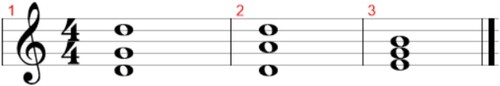
Figure A2. An example of two bars playing the same chord, but with the second one shortening the duration the chord is being played. The distance between these two bars is 1 since the onset of the two chords and the chords are the same, but the rest in the second bar creates a difference between them.
Figure A3. An example of two bars with the same chord played all along but with different onsets. The distance between these two bars is 3 since, even though the same note would be heard all along, the first bar has a unique onset and the second one has four onsets, on the tempo. Thus, the first onset is common to the two bars and does not increase
, but the following three are only found in the second bar and each of them increments the distance by 1.
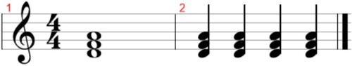
Figure A4. The titles ordered according to their score (only the first 20 lowest ones are depicted here). The blue dots correspond to the
scores, which are obtained by computing the average distance between songs from a given decade. The blue bars show the standard deviation around this average distance. The bars in red represent the number of songs who appeared for the first time in the corresponding decade. One can see that all the lowest scores correspond to song covers, as to be expected.
Appendix 3.
Extra figures
In this appendix, we provide some extra figures to complete the study presented in Section 4. We start by providing the first scores of the different features: title in Figure , decade in Figure , genre in Figure , and type in Figure . We recall that the first
scores for year can be found in Figure while those of artist are showcased in Figure with different limits on the minimal number of songs per artist.
Figure A5. The seven decades available in the dataset ordered according to their score. The blue dots correspond to the
scores, which are obtained by computing the average distance between songs from a given decade. The blue bars show the standard deviation around this average distance. The bars in red represent the number of songs who appeared for the first time in the corresponding decade. Although no decade has a notably lower score than the next one, the decades past the year 2000 have higher score, meaning that they have a (slightly) richer variety of patterns.
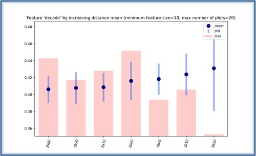
Figure A6. The genres ordered according to their score (only the first 20 lowest ones are depicted here). The blue dots correspond to the
scores, which are obtained by computing the average distance between songs with a given genre. The blue bars show the standard deviation around this average distance. The bars in red represent the number of songs with the corresponding genre. It is worth observing that the second lower
score, corresponding to the genre ‘progressive pop’, has a rather large size compared to the rest of the other genres with low score.
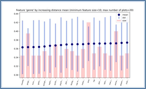
Figure A7. The types ordered according to their score (only the first 20 lowest ones are depicted here). The blue dots correspond to the
scores, which are obtained by computing the average distance between songs with a given type. The blue bars show the standard deviation around this average distance. The bars in red represent the number of songs with the corresponding specific type. Interestingly, most types refer to genre adjectives (such as ‘gothic’, ‘acid’, ‘novelty’) rather than genre categories (such as ‘rock’ or ‘rap’) and two types appear to have a low score but a rather large size (compared to the rest): ‘emo’ and ‘art’.
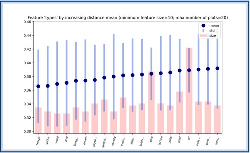
After showing the score for all features, we now show the
scores of our clustering methods (apart from the feature title, for which we do not have enough repetitions to have a meaningful interpretation of the clusters with a low
score). While the first
scores of the feature year can be found earlier, in Figure , we provide here the first
scores of artist (in Figure ), genre (in Figure ), and type (in Figure ). We further show the songs of cluster 471 of our algorithm, which appears as one of the lowest scores in all previous figures.
Figure A8. Clusters ordered according to their score with regards to the feature artist (only depicting the 20 lowest scores). The blue dots represent the average score of the cluster, the blue bars represent the standard deviation around this score and the red bars represent the sizes of the clusters. This figure needs to be combined with a representation of the clusters in order to appreciate its results. The cluster numbered 471 (thus one of the five with the lowest score) is represented in Figure .
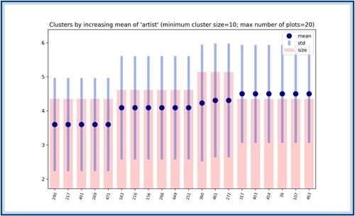
Figure A9. Clusters ordered according to their score with regards to the feature genre (only depicting the 20 lowest scores). The blue dots represent the average score of the cluster, the blue bars represent the standard deviation around this score and the red bars represent the sizes of the clusters. This figure needs to be combined with a representation of the clusters in order to appreciate its results. The cluster numbered 471 (thus the one with the lowest score) is represented in Figure .
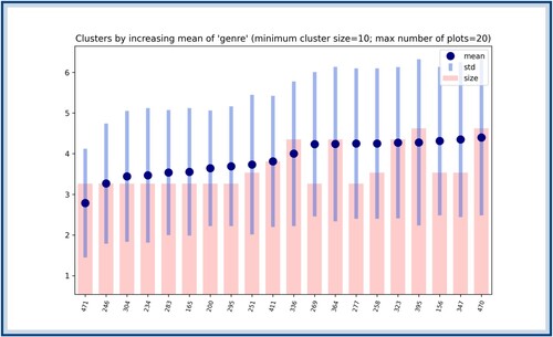
Figure A10. Clusters ordered according to their score with regards to the feature type (only depicting the 20 lowest scores). The blue dots represent the average score of the cluster, the blue bars represent the standard deviation around this score and the red bars represent the sizes of the clusters. This figure needs to be combined with a representation of the clusters in order to appreciate its results. The cluster numbered 471 (thus the one with the second lowest score) is represented in Figure .
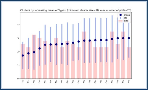
Figure A11. A representation of the cluster numbered 471, having a low score in Figures –. As one can see, all songs have a similar genre (somewhere between ‘pop’ and ‘rock’), however the artist similarity only arises from two of the songs being from HENREY MANCINI. This means that to find finer similarities between songs of the same artist, we need to lower the minimal size of a cluster to less than 10, as it was done in Figure ; in particular, this is how we managed to find the similarity between songs of LINKIN PARK from Figure (note that there are less than 10 songs in the top two clusters).
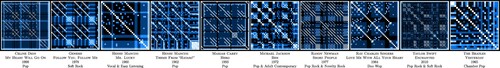
We conclude this appendix with a study on the use of the different clustering algorithms: Agglomerative Clustering, Spectral Clustering, and K-Medians. To do so, we ran two experiments:
we apply each of the clustering algorithms once and output 20 clusters.
we apply each clustering algorithm recursively, as described in Algorithm 1, using the aforementioned parameters (
The general statistics of the clusters in the first experiment are shown in Figure . As one can see, K-Medians seems to be the best algorithm to use in that case since it provides the most balanced clusters, and Spectral Clustering fails to extract relevant information since it basically splits the dataset into one giant cluster and 19 leftover clusters (in fact 17 of these clusters are singleton and do not show in Figure ). The general statistics of the clusters in the second experiment are shown in Figure and are less readable than in the previous case. However, it is worth noting that 419 out of 1047 clusters () are singleton in the case of K-Medians, while only 48 out of 527 clusters (
) are singleton in the case of Agglomerative Clustering. Spectral Clustering outputs 37 singletons out of a total of 516 clusters (
).
Figure A12. A representation of the statistics of the clusters when applying the three algorithms and outputting 20 clusters. The blue dots represent the average distance between songs of a cluster, the blue bars the standard deviation of these distances, and the red bars the sizes of the clusters. At the top is the output when applying the Agglomerative Clustering, the bottom left figure corresponds to the K-Medians clustering and the bottom right figure corresponds to the Spectral Clustering. As one can see, K-Medians provides a balanced set of clusters, none of them being a singleton, while Spectral Clustering provides only three non-singleton clusters and one with almost all the songs. These figures seem to show that K-Medians is the best algorithm, however, when applied recursively to reduce the sizes of the clusters, it tends to create a lot of singleton clusters and provides less interesting results than Agglomerative Clustering (see Figure ).
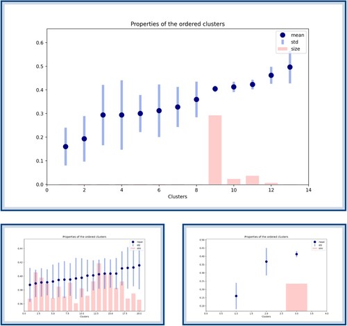
Figure A13. A representation of the statistics of the clusters when applying the three algorithms until all clusters have size at most 15. The blue dots represent the average distance between songs of a cluster, the blue bars the standard deviation of these distances, and the red bars the sizes of the clusters. At the top is the output when applying the Agglomerative Clustering, the bottom left figure corresponds to the K-Medians clustering and the bottom right figure corresponds to the Spectral Clustering. These figures are less readable than those of Figure and it is worth stating another output of the algorithm for each cases, counting the total number of clusters and singletons: 527 clusters including 48 singletons for Agglomerative Clustering, 1047 clusters including 419 singletons for K-Medians, and 516 clusters including 37 singletons for Spectral Clustering. Combinng the above figure with Figure shows that Agglomerative Clustering is the most balanced algorithm to consider here and thus explains our choice in Section 4.2.
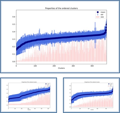
Given the above results, the choice of Agglomerative Clustering came as a desire to balance the output of the two previous experiments and further made sense with regard to the tree-like structure of the songs as shown in Figure .