Who will dominate the global fossil fuel trade?

Abstract

Fossil fuels are not distributed evenly throughout the world, and hence the countries rely heavily on international trade to secure energy supply. Characterization of the energy trade network is needed to conduct long-term assessments of energy security. This study proposes a modeling framework to assess the evolution of energy trade under current conditions as well as under future scenarios up to 2050. The total trade of each country is estimated with trade predictive models (TPMs) using key variables. Subsequently, a matrix-balancing method (RAS) is used to estimate the annual bilateral trades. The projected energy trade network in 2050 varies under each shared socioeconomic pathway (SSP) of the future, with annual fossil fuel global trades among countries ranging between 538 and 215 EJ. Canada, USA, Venezuela, and China are projected to dominate the global trade network, with Canada-USA remaining the most dominant fossil fuel trade link up to 2050.

KEYWORDS:

• Global trade networks
• energy trade modeling
• RAS method
• trade predictive models

1. Introduction

Access to sufficient and affordable energy resources is essential to improve human welfare and raise living standards worldwide. In spite of the current global trend towards renewable energy sources, fossil fuels including oil, natural gas, and coal are still the dominant sources (84.7%) of energy (BP Statistical Review of World Energy, 2019), mainly because of their affordability and availability (Kumar et al., 2011). Since globalization has become a prominent factor in the world economy, global energy trade has played a substantial role in energy supply security by redistributing energy throughout the world (Chen & Chen, 2011). The global energy trade network is a complex system, mainly due to the complexity of the relations among the numerous participants in the market (Gao et al., 2015), and the influence of several controllable and uncontrollable factors on the energy trades. In addition, energy trade policies are subject to political pressures as they are mostly implemented through political processes (Zelby & Groten, 1990) that might limit trade due to, e.g. political sanctions. In addition to concerns about the potential impact of trade barriers and political instability on energy trade, one of the major concerns is the balance between demand increase and resource availability. Therefore, the capability of the international energy market to supply the global demand, in relation to the availability and distribution of resources, might be an important challenge in the near future.

A large body of literature offers an empirical analysis to understand the energy trade network (An et al., 2014; Bale et al., 2015; Fracasso et al., 2018; Gao et al., 2015; Geng et al., 2014; Ji et al., 2014; Lu et al., 2014; Ruzzenenti et al., 2015; Sun et al., 2012; Zhang et al., 2014; Zhong et al., 2014), but it is still less than exhaustive. First, the existing studies usually employ a few select techniques such as complex network theory, which is an effective tool to analyze the features and properties of trade networks, but do not propose a methodology to (i) model the global energy distribution from exporters to importers or (ii) characterize the behavior of energy fluxes over time. Second, the capability of the global market to keep the global energy trade network balanced over time is rarely discussed (Distefano et al., 2020). Third, most studies are carried out only at local or regional scales, without providing country-level details. Fourth, to the best of our knowledge, no studies have been carried out to project the future global energy trade network in a comprehensive country-based and quantitative manner. However, a few studies provide a perspective with respect to the future of the energy market (Feng et al., 2017; Holz et al., 2015; Kumar et al., 2011; Paltsev et al., 2011; Sharmina et al., 2017), but these have a limited scope by focusing on selected countries and do not propose a methodology to investigate bilateral energy trade between countries under future scenarios.

With regard to bilateral international trade, gravity law models (GLMs) have been successful in explaining trade fluxes (Anderson, 1979). GLMs, which are multivariate regression models, are able to estimate the bilateral trade fluxes between two nodes (Tamea et al., 2014) and have been used to estimate trade in a variety of areas in which the main focus has been on modeling node-to-node trade flows. However, when it comes to modeling the global trade network, the node-to-node approach is considerably constrained; one of the main limitations is the negligence of each node’s overall trade potential within the global market. As a result, GLMs may underestimate the total global flows (Tuninetti et al., 2017), and the total inflow-outflow of each node may exceed their trade capacity in an interconnected trade network. Another limitation of the node-to-node approach is the low accuracy of the overall trade distribution in a network, which is mainly an outcome of the first constraint. In fact, by following the node-to-node approach, bilateral trades are estimated regardless of the other multilateral trades of a node. Thus, trade distributions cannot be accurately estimated because the trade’s potential and priorities are not considered. Utilizing input–output (IO) techniques (McDougall, 1999; Parikh, 1979; Toh, 1998) for updating and balancing the global trade, based on the total capacity of exports and imports, could be one solution toward improved understanding of the behavior of trade networks with respect to the node’s overall trade potential. The RAS method is the best known and widely used IO technique, due to its operational simplicity (Toh, 1998), to reconcile the bilateral trade flows for updating the input–output tables (IOTs) (Lahr & De Mesnard, 2004; Wiebe & Lenzen, 2016) with the constraints respected by targeting marginal (node) totals (Jackson & Murray, 2004). Updating an IOT provides the ability to investigate the evolution of a trade network (Dietzenbacher & Hoekstra, 2002; Tarancón & Rio, 2005), analyze trade relationships, and study the development, destruction, and substitution of trade links (Dietzenbacher & Hoekstra, 2002).

Several studies link IO techniques and GLMs (Aichele & Felbermayr, 2015; Caliendo & Parro, 2015; Guilhoto et al., 2015; Noguera, 2012; Sarker & Jayasinghe, 2007; Sartori et al., 2017), where GLMs are sometimes used to estimate the bilateral trades (node-to-node) as the initial inputs of tables (Duarte et al., 2018; Sargento et al., 2012). Recently, Distefano et al. (2020) assessed the performance of GLMs and the RAS method in the estimation of bilateral trades and summarized the pros and cons of each approach. However, a modeling approach is needed for the global energy trade to explain the distributions of energy in the global network and investigate how the network remains balanced when the characteristics of the network and nodes change. This study aims to address the abovementioned issues, and in particular, it contributes to the existing literature the following: (i) development of a novel modeling framework for characterizing the global energy trade network under current and projected future conditions by employing and combining GLM-based regression models (to estimate total energy trade of each node) and RAS method (to estimate the bi-lateral energy fluxes) to benefit from the strengths of both GLM and RAS methods; (ii) a new characterization of the global fossil fuel energy trade networks, along with quantification of the bilateral trades, under future shared socioeconomic pathways (SSPs); and (iii) investigation of the potential evolving communities (clusters) of countries, forming sub-networks within the global trade networks.

2. Data and methods

The overall research methodology is summarized as follows: (i) significant energy trade links were identified in the bilateral trade network. Considering all countries (222) means 49,062 potential trade links; however, preliminary investigations revealed that 90% of the global energy trade from 2000 to 2016 occurred through only 1,185 links. Therefore, the significant exporting and importing countries (network nodes), along with trade links, were identified from historical trade data to construct the trade network. As regression models can generally preserve the mean of the dependent variable, GLMs are better suited to estimate the total flux from (or into) a county to (or from) the rest of the world. However, as the geographical distance (as the friction factor of GLM) is not included in the proposed models formation, we call them the Trade Predictive Model (TPM); (ii) a list of potential factors that affect the global energy trade was prepared based on data availability, as well as prior knowledge from previous food and energy trade modeling studies; (iii) descriptive TPMs were developed for each node to estimate its total annual export to, and import from, the rest of the world using the identified factors as independent model variables (predictors); and (iv) using the predicted total annual exports and imports of each node, the RAS method was used to reconcile the constructed trade matrices and estimate the bi-lateral fluxes of energy of each network node (country). The whole modeling approach was developed based on the historical period (2000–2016) for the baseline analysis, due to the availability of bilateral energy trade data, and the possible futures of the global energy trade were then projected based on selected future global scenarios (details provided in the following sections).

2.1. Data

Global energy trade data were obtained from UN Comtrade (2019) which is the freely accessible United Nations International Trade Statistics Database (http://resourcetrade.earth). Additional data for all countries were also obtained from the U.S. Energy Information Administration (EIA) database (US EIA, 2020), including population, gross domestic product (GDP), energy production, and energy consumption. This study focuses on the primary energy commodities of oil, natural gas, and coal. Energy production, consumption, and trade were converted to gigajoules (GJ) separately for oil, natural gas, and coal so all three primary sources had the same energy units and could be summed up in one quantity. A comprehensive energy conversion calculator tool, EIA Energy Conversion Calculator (2020) was used for the energy conversions. Table 1 summarizes the data used in this study.

TABLE 1. Energy related data used in this study, along with their original reported units.

Data	Source	Unit
National Population*	EIA	Capita
Global Population*	EIA	Capita
GDP*	EIA	Billion $2010 PPP^a
National fossil fuel energy production*	EIA	Tera joules
Global fossil fuel energy production*	EIA	Tera joules
National fossil fuel energy consumption*	EIA	Tera joules
Global fossil fuel energy consumption*	EIA	Tera joules
Energy intensity*	EIA	Btu^b/$2010 GDP PPP
National energy production of other sources of energy*	EIA	Quad Btu
Bilateral fossil fuel energy trades	UN Comtrade	Kilogram (Weight)
Total export-import**	EIA	bbl ^c

^a PPP: Purchasing Power Parity; ^bBtu: British thermal unit; ^cbbl: Barrel, *Independent variables considered for the TPMs, **Dependent variable in the TPMs.

2.2. Network construction

The global energy trades can be viewed as a network of bilateral trade flows whose structure is determined by participation of several nodes, which yield an Energy Trade Matrix (ETM). In the proposed modeling approach, 77 countries (nodes) were selected, which on average represented 93% of the fossil fuel energy trade during the study period (1993–2016). The 77 selected nodes include 51 exporters and 59 importers; 26 are only-importer, 18 only-exporter, and 33 exporter-importer. The 77 nodes (countries) created a maximum of 2,976 links, which were not all active in the network according to the trade data. For instance, in the USA-Iran trade link, both countries are major players in the global energy trade network, but there has been no energy trade through this link due to historical political conflicts. A subsequent filter was applied, similar to the approach followed by Tuninetti et al. (2017) for food trade networks, by considering a link to be active only if it was active for more than 50% of the time (9 years out of the simulation period of 17 years) and if the volume of trade was at least 0.05% of the average of all global fluxes. This filter was applied to avoid cluttering the network with insignificant links that would cause excessive data noise without adding much value to the objective of capturing the global energy trade (Tuninetti et al., 2017). The adopted thresholds led to keeping only 1,185 active trade links, which carried 90% of the energy trade in the study period (Table S1). The trade in the inactive links was considered zero in the network in all years. Additional assumptions included a fixed network topology as well as trade links maintaining their condition (active or inactive) over the baseline period.

2.3. Trade predictive models

GLM is a regression-based model, often used to estimate the fluxes occurring in trade networks (Bergstrand, 1985). For decades, GLMs have been reasonably successful at explaining the bilateral flows of different types of trade (Distefano et al., 2020). The original GLM formulation is inspired by Newton’s universal law of gravity: ‘The attraction between two objects depends on the mass of these objects’ (Anderson, 1979). In this study, we developed GLM-based models (coded in Matlab) to describe the relationships between the total energy outflows (exports of a country to the rest of the world) as a dependent variable and a set of indicators as independent variables (Country to World or C_i_W models; Equation 1). Similarly, the imports of each country (W_C_j models) were developed (Equation 2). However, in this proposed type of representation there is no need to consider the geographical distance between a country and a central node that represents the global market. Therefore, we call the proposed multivariate regression model as TPM to simulate the total exports and imports of each node of the network. The TPMs were formed as a linear regression between the logarithms of trade and explanatory variables (Tamea et al., 2014), and

C_i_W models (1) $Log(F_{i,g})={\beta }_1+{\beta }_{2}Log{\text{v}}_1+{\beta }_{3}Log{\text{v}}_2+{\beta }_{4}Log{\text{v}}_3+\dots$(1)

W_C_j models (2) $Log(F_{g,j})={\beta }_1+{\beta }_{2}Log{\text{v}}_1+{\beta }_{3}Log{\text{v}}_2+{\beta }_{4}Log{\text{v}}_3+\dots$(2) where F_i,g is the energy flow from the exporter node i to the global market g, and F_g,j is the energy flow from the global market g to the importer node j. βs are the model parameters interpreted as the regression coefficients, and v_i is a model independent variable (provided in Table 1). For g, global data were used and the data of nodes i and j were always excluded. The robust linear regression method (DuMouchel & O’Brien, 1992) was employed to estimate the regression calibration parameters with the best performance in fitting the data. As fitting one regression model for all countries is not logical, 110 multivariate regression TPMs were developed for the selected 77 countries in the study period (1993–2016). First, the TPMs of 51 exporters and 59 importers were developed/calibrated for the period 1993–2009 (17 years annual data or 70% calibration sample size) to estimate the sets of parameters. The TPMs were then validated for the 2010–2016 period. It is recognized that the calibration and validation split samples are small; however, several studies simply employed the entire record for developing such trade models without split samples (Tamea et al., 2014; Tuninetti et al., 2017). Therefore, the approach adopted in this study adds another validation layer, admittedly limited, to ensure reasonable model reliability and similar to what was done by Abdelkader et al. (2018).

To obtain the optimum number and the best set of independent variables for the export and import TPM models, country to world and world to country, the stepwise regression technique was implemented through three different alternative regression approaches (I, II, and III). In regression approach (I), the export of country i, as a dependent variable, was regressed against an independent variable v1. This was repeated for all export countries with the same variable v1, then tried with each of the other independent variables: v2, … v9. The variable with the best corresponding overall result – median of the results of all exporters – was labeled as the best single variable and kept for the next step. In step 2, the best second variable, v2, was sought in the same way among the remaining eight independent variables and was added to v1 to form a model with the best two variables, and so on until the best models with an increasing number of variables were formed. At all steps, the decision was made based on the median performance over all countries to have models with the same set of independent variables for all countries. Also, it is important to note that all country models with, for example, v1 and v2 are the best two-variable models that include the best single-variable identified in step 1. The best three-variable models include the same two variables identified in the best two-variable models, and so on. In regression approach (II), the best two-variable models were obtained regardless of the best single-variable. This means that the single-variable model for all countries might include, e.g. v4 but the best two-variable models can include v1 and v5 for all countries. The same thing applies to all models with more variables. In other words, the regression algorithm was free to select a set among all nine independent variables, as long as the selected set applies to all export countries. In regression approach (III), the regression was free to select the best sets and variables for every country individually, so, the best two-variable for country i can be, for example, v1 and v3, but for country k, they are v2 and v7.

The overall performance of TPMs in each step was evaluated, for the calibration (1993–2009) and validation (2010–2016) periods, using two quantitative statistics: R² and Mean Absolute Relative Error (MARE) (Equations S1 and S2). Accordingly, the performance of the TPMs was evaluated for each node, and the median of all results based on R² and MARE values reported. As the optimum number and best set of variables for each node were obtained, the performances of TPMs were then individually evaluated with respect to the estimation of the total volumes of energy flow using percent bias (PBIAS) (Equation 3) to characterize any over/underestimation. (3) $PBIAS(\mathrm{\%})=\frac{{\sum }_{i=1}^n({Q_{obs}}_i-Q_{si{m}_i})}{{\sum }_{i=1}^n({Q_{obs}}_i)}\times 100$(3) where $Q_{obs}$ is the observed energy flows, $Q_{sim}$ is the simulated energy flow, $\overline{Q_{obs}}$ is the mean of observed energy flows, and $\overline{Q_{sim}}$ is the mean of simulated energy flows. MARE represents the average affinity of the simulated flows and ranges from 0 to +∞, indicating relative percent error in the model performance; R² is the proportion of the variance explained by the independent variables in the TPMs, and ranges from 0.0–1.0 where 1.0 indicates the highest accuracy; and PBIAS is the average of the bias in the simulated energy flows and ranges from −∞ to +∞, indicating overestimation and underestimation of the energy flow volumes, respectively (Gupta et al., 1999).

2.4. RAS – energy trade matrix balancing technique

The RAS method, which is a matrix balancing technique (Wiebe & Lenzen, 2016), was utilized to construct and populate the global energy trade network, reconcile the ETMs, and estimate the mutual energy trade between each pair of nodes.

The modeling approach developed (Figure 1) includes the following three steps:

1. The outputs of the TPMs (the total energy export-import of countries) were used as inputs to the annual ETM shown in Figure 2, as the table targets;

2. The table cells F_i,j were filled by numbers as initial conditions, required for the initiation of the RAS method. Different initial conditions were also considered, as explained below; and

3. The iterative procedures of the RAS method were conducted, and the resulting bilateral trade flow of each link was assessed when the table reached a balance (i.e. the estimated total exports and imports matched with the targets specified in step 1).

Figure 1. Schematic representation of the global energy trade modeling approach.

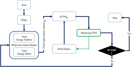
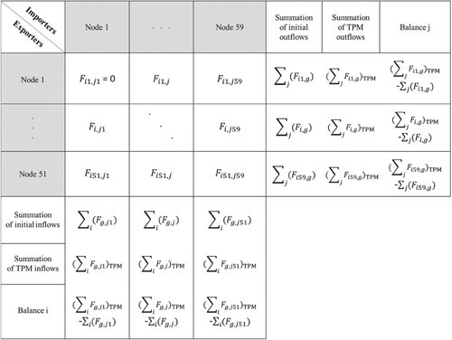
Figure 2. Structure of the Energy Trade Matrices (ETMs), based on 51 exporters and 59 importers. The gray cells indicate the countries involved in the bilateral trade. The cells with the rows and columns summations refer to the total export and import flows of each country, respectively.

Global bilateral trade data are available only after 2000, and therefore the period 2000–2016 was considered for the RAS application. As shown in Figure 1, the above process was repeated n times for the n years of the study period, with an ETM constructed for each year. In the process of balancing the ETMs, the accuracy of flow distribution is highly dependent on the weights and topology of the initial conditions. Five different initial conditions were considered to initiate the RAS method and generate the bilateral flows: (A) for each year of the study period, 1000 sets of random numbers (1000 tables) were generated as alternative initial conditions using the Latin hypercube sampling method (Stein, 1987), and the best set of the 1000, based on the simulated bilateral flows, was identified; (B) all initial F_i,j were given the same value of ‘1.0’ to provide the same initial weight to all trade links; (C) values of one over the geographical distance between each pair of nodes were used as the initial inputs, where the priority of trades emphasizes closer nodes (Anderson, 1979; Bergstrand, 1985); (D) the actual bilateral flows of the first year of the simulation period $(F_{i,j}{)}_{obs,2000}$were used as the initial conditions of the table, and in subsequent years the balanced (modeled) bilateral energy trade flows of the preceding year were used, and (E) the node-to-node approach was used to estimate the annual initial conditions of the ETM where we develop the commonly used GLMs, as incorporated the factor of geographical distance between each pair of countries, for the number of active links (1185).

Based on the findings, one of the abovementioned five conditions will be used to produce an annual energy trade table. For each year, one table (Figure 2) was created, representing the global energy trade network of the corresponding year, where the rows and columns represent the outflows and inflows of nodes, respectively.

The RAS method is explained in more detail in McDougall (1999), Toh (1998), UN Statistical Division (1999), Parikh (1979), and Mínguez et al. (2009). Balanced matrices for each year were obtained with an iterative procedure that progressively updates the initial inputs until the error difference between two consecutive steps, as an objective function, is minimized. This method was validated in this study using the energy bilateral trade data of the global energy market available from the UN Comtrade (2019). The performance of the RAS method was assessed using R² to evaluate a node’s energy trade flux simulations.

2.5. Future projections of global energy trade

Global energy trade networks were projected for the study period 2017–2050. This projection was conducted under future scenarios based on Shared Socioeconomic Pathways (SSPs) (O’Neill et al., 2017), which project the future population, GDP, annual fossil fuel consumption, and production (Table S2). The projected population and GDP, on 5-year intervals, come from the SSP database (Cuaresma, 2017; Samir & Lutz, 2017) at the country scale, and the energy data, with a 10-year interval, are the outcome of the integrated assessment model (IAM) at the regional scale (Calvin et al., 2017; Fricko et al., 2017; Fujimori et al., 2017; Kriegler et al., 2017; Van Vuuren et al., 2017). The International Institute for Applied Systems Analysis (IIASA) divides the whole world into five regions (OECD, REF, ASIA, MAF, and LAM); more details regarding the regional aggregation can be found in the IIASA database (IIASA, 2020). The proposed country-based modeling framework includes updating the ETMs over time within annual intervals. Therefore, the regional energy data (IIASA projections) were disaggregated into a country-based scale and the 5- and 10-year intervals into annual intervals. The regional energy data (production and consumption) were broken down to the country-based scale according to the country’s share in the corresponding region in the baseline period. The 5- and 10-year interval data were disaggregated to annual data based on linear interpolation.

This study focuses on five SSPs (IIASA, 2020) that are based on RCP4.5, one of the four representative concentration pathways (RCPs) forcing targets, based on the data availability. Accordingly, the TPMs were developed under the future five SSPs, and the RAS method was used in a way similar to that conducted for the baseline period to project the bilateral flows of energy across the global network. The only difference in the RAS method for future projection is the first year of initial conditions, which is the year 2016, instead of 2000 for the baseline period. The calibrated TPMs also used the future-projected variables to estimate the future total trade fluxes. The inactive links, which were forced to be zero in the baseline period, were all weighted with a small value of 1.0 to have a chance to grow under the future scenarios, e.g. in the case that a minor country increases its production in the future. The narratives for each SSP are described in detail in Riahi et al. (2017) and Bauer et al. (2017).

3. Results and analysis

3.1. Performance assessment of the developed TPMs

The investigation of the three possible approaches of the regression models (explained in Section S1), led to the implementation of approach (III) in the analysis. Accordingly, the TPMs, including four independent variables that vary across different countries, resulted in the best approach for modeling both the export (C_i_W) and the import (W_C_j) TPMs. As the number of inputs increase, the TPM performance (average performance across all countries) improves during model calibration; however, there is a turning point beyond four inputs in the validation period (Figure S1). The TPMs have an average satisfactory performance across all importer and exporter countries, with R² values of 0.51 and 0.55 and MARE values of 4.8 and 4.6% for importers and exporters, respectively.

In stepwise regression approaches (I) and (II) for the 51 exporters (C_i_W) and 59 importers (W_C_j), the overall performance of the TPMs in the validation period is not satisfactory (R² and MARE) and does not show an optimum number of input variables (Figure S1, the panels in the upper and middle rows). This can be attributed to the need for different set of inputs for different countries, which is achieved in TPMs of approach (III). According to the stepwise regression results for both C_i_W and W_C_j models, the best set of four input variables, out of nine (Table 1), was obtained for every exporter-importer node (the bottom panels of Figure S1 show the best performance achieved with four independent variables). Figure S2 shows the global median values of MAREs based on approach (III), with the distribution of overestimation and underestimation in the validation period. The results indicate the TPMs maintain their stable performance over the validation period for both importers and exporters.

The TPMs were used in this study to model and characterize the total fossil fuel trade (imports and exports) of major players with the rest of the world; therefore, it is important to investigate the PBIAS of such models. Figure S3 shows the performance of individual exporter/importer TPMs using approach (III) in the validation period. The poorest performance of the TPMs belongs to North Korea with a PBIAS of −35.5%. Canada and Venezuela also have less accurate models, compared to other exporters, with PBIAS values of −27.3 and −22.3%, respectively. Such negative values of PBIAS indicate an overestimation of energy exports of these countries. These less accurate estimations are probably due to the absence of some unknown variables that are not included in the TPMs or to the number of selected variables. For instance, after a focused consideration of these particular countries, it is concluded that the TPM developed for Canada performs better in the validation period, with a PBIAS of 16%, when it includes five variables; this is not the case for Venezuela, for which adding or removing variables does not improve the model performance. Similarly, there is a less satisfactory performance for six importers – Colombia, Egypt, Hong Kong, Pakistan, Tunisia, and Turkey – with PBIAS values of 22.5, −23.2, −24.9, 22.2, 40.3, and 38.4%, respectively. As shown in Figure S3, the performance of models for most countries, with a few exceptions, is between +10 and −10%, which is satisfactory. Additionally, the well known F-test was used to evaluate significance of the influence of independent variables on the dependent variable (Shen & Faraway, 2004). The results indicate that the developed TPMs are significant for 42 exporters (82%) with P-value < 0.1 including 40 exporters (78%) with a P-value < 0.05. Similarly, 47 importer TPMs (82%) have a P-value < 0.1, including 41 (70%) with a P-value < 0.05. However, the P-value > 0.1 for 9 exporter and 11 importer TPMs, which could be attributed to the small sample size of data. The highest P-values of 0.4, 0.41, and 0.42 belong to the three exporter TPMs of Yemen, Ukraine, and Egypt, and P-values of 0.38 for the importer TPM of Philippines. As shown in Figure S3, there are a few TPMs with 0.26 > P-values > 0.1 which include the exporter TPMs of Poland, Sweden, United Arab Emirates, Bahrain, and Nigeria, and the importer TPMs of Denmark, Brazil, Slovakia, Japan, Bangladesh, United States, Mexico, Canada, Belarus, Hungary, and Israel.

3.2. Performance assessment of the bi-lateral energy flow modeling (RAS)

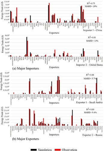
Our investigation regarding the best possible approach to construct the bilateral energy flows reveals that using the observed trade values of the first year of the simulation period (condition D, Section 2.4) as initial conditions lead to the best results (Figure S4), compared to the other approaches used in the literature. The simulation accuracy starts with an R² value of 0.98 in year 2 and decreases over time until it reaches 0.70 in year 17. Note that the performance of a model with an R² value >0.95 can be maintained if the observed trade values of the past year or two are used. This can be adopted if characterization of the trade network over the historical period or a forecast of one- or two-year lead time is desired. However, we used the initial values of the first year of the simulation period to enable reconstruction of future projections of the trade network over several years. The performance of the RAS method was assessed as an average over all cells in the ETM, which means an average value over the global trade network. The performance of the RAS method for each country is shown in Figure S5. The energy trade is predicted with acceptable accuracy for 31 exporter nodes (60% of the network) with R²> 0.6, including 19 nodes (36%) with R²> 0.8. The results also show weak performance in capturing the trade patterns for seven nodes (13%; Argentina, Ukraine, Yemen, India, Egypt, China, and Azerbaijan), with a total network trade flux share of 3.2% and R²< 0.4. For the importers, the accuracy of the prediction for 36 nodes (61%) is good with R²> 0.6, including 27 nodes (45%) with R²> 0.8; for 12 nodes (20%; Nigeria, Colombia, Switzerland, Yemen, Bangladesh, Malta, Argentina, Panama, Chile, Australia, New Zealand, and Portugal), the accuracy is low with R²< 0.4, with total network share of 3.6%. The results show the performance of the RAS method in modeling energy trade is better for major players of the global energy network, which have a larger global market share. The RAS performance is very good for 18 major exporters, which carry 80% of the network energy supply and have an average R² of 0.79, and for 15 major importers, which carry 81% of the network energy demand and have an average R² of 0.80. The results also indicate weak performance of the RAS method for countries with a small global market share. To more closely examine the performance of the RAS method, Figure 3 shows, as examples, its performance in the estimation of the node’s energy trade values for two major exporters (Saudi Arabia and Russia) and two major importers (the United States and China) in the last year of the simulation period (2016).

Figure 3. Performance of the RAS method with respect to the simulation of energy flux for (a) two major importers and (b) two major exporters in 2016.

3.3. Analysis of the key variables influencing the energy trade

Based on our methodology, each country has only four selected influential variables that substantially affect its energy trade (Figure S6). For example, Saudi Arabia’s energy exports are mainly governed by its national GDP, its fossil fuel production, global fuel production, and global consumption. The first two variables logically reflect the country’s economic reliance on its energy exports, which are only limited by the global market demand (represented by the latter two variables). Canada, as an exporter, shares with Saudi Arabia the importance of national and global fuel production as variables, but is unique in other aspects. As a major energy consumer and a developed country, Canada’s energy exports are affected by its national energy intensity and reliance on other sources of energy (e.g. hydro, nuclear, wind). Note that an exporter-and-importer country such as Canada can have different variables affecting its imports and exports. For example, the national GDP, reflecting industrial development and economic expansion, is an important factor for Canada’s imports of fossil fuel energy (Figure S6).

Among a total of nine variables, national production of fossil fuel is globally the most used variable in the TPMs of exporters, where it is included in 29 exporter nodes (57% out of 51 exporters). Three other variables – national population, national energy production of other sources of energy, and global fossil fuel energy consumption – are also used in TPMs of 28, 27, and 26 exporter nodes, respectively (Figure S7). In addition, energy intensity is the least influential variable, being used for only 15 exporter nodes. With regard to importer countries, note that all variables are influential in the global market, where national GDP is the most used, affecting 28 importer nodes (47%). The role each variable plays in increasing/decreasing the energy export/import of the countries was analyzed according to their signs in the regression models (TPMs) (Figure S8). Interestingly, a mixed signal effect of all variables globally is evident. For example, global production of fossil fuels has an increasing effect on the exports of 10 exporters but a decreasing effect on 12 other exporters. On the other hand, the same variable has an increasing effect on the imports of 13 countries and a decreasing effect on another 13 importers (Figure S8).

3.4. Future scenarios of the global energy trade

The two-step modeling approach developed in this study (TPMs, followed by RAS) was adopted to project the global energy trade network under five different SSPs. Figure 4 shows the projected total global fossil fuel energy trade under different SSPs for the period from 2017 to 2050. In SSP5, a world of rapid and unconstrained growth in economic output and energy use (Keilman, 2020), the global energy consumption and production are at their highest levels, which leads to fast growth in the global energy trade between energy suppliers and importers.

Figure 4. Projected annual fossil fuel energy trade at the global scale.

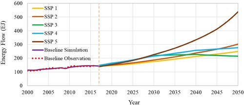
The results show a sharp increase of the energy traded under scenario SSP5 (Figure 4) to a value of 538 EJ in 2050 – a 260% increase compared to the 148 EJ in 2016. The rank of SSPs in the corresponding projected global energy trade varies over time, but in 2050, SSP2, SSP4, SSP1, and SSP3 (in that order) come after SSP5. In the case of SSP3, a fragmented world of resurgent nationalism (Keilman, 2020), countries focus on domestic and regional issues (Riahi et al., 2017) and decrease their production and consumption, which leads to the lowest global energy trade (215 EJ). However, trade still increases by 45% compared to 2016 levels, over a period of 34 years.

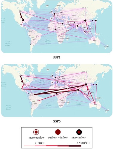
Figure 5 is the topological visualization of the projected global energy trade network in 2050, using the Flowmap tool (Boyandin, 2020). We show here SSP1 and SSP5 as two distinct scenarios; the remaining scenarios are shown in Figure S11. The Canada-USA link is projected to continue as the strongest bilateral trade link under all SSPs, with Venezuela’s exports to China and India emerging as equally strong under SSP5. The gentle increasing trend of energy trade under SSP3 and SSP4 (Figure 4) is obviously caused by declining imports of China and India – the world’s largest importers under these two scenarios (Figure S11).

Figure 5. Visualization of the projected global fossil fuel energy trade network at the country scale under SSP1 and SSP5 in 2050 (remaining scenarios shown in Figure S11).

Currently, the top three exporters of fossil fuel energy are Russia, Australia, and Saudi Arabia, with Russia mostly dominating the European trade flows (Figure 6a). According to our analysis, the 2016 energy network exhibits four main communities (sub-networks) containing nodes that are more densely connected together than to the rest of the network. Community detection was carried out using Gephi (https://gephi.org/), a network visualization and exploration software. The algorithm for community detection is based on optimizing the network modularity (the strength of division of a network into modules) according to the approach proposed by Blondel et al. (2008). At the beginning, the number of communities equals the number of countries. The algorithm then iteratively merges communities that optimize the modularity of the network. The energy trade network has a modularity of 0.43, which is an indicator of significant modularity with four communities.

Figure 6. Networks of fossil fuel energy trade in (a) 2016 and 2050 under (b) SSP1 (green road) and (c) SSP5 (fossil fuels) scenarios. Nodes are colored according to their community evaluated with the modularity optimization algorithm. For each community, the percentage of included nodes is shown in the legend. Node size is proportional to export flow, and the top three exporters of each scenario are represented in the legend. Link color is in accordance with source nodes to highlight the energy flow sources of each community.

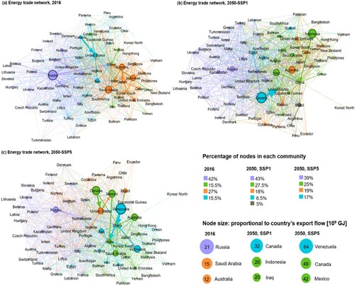
In the current network, Russia dominates the biggest community, including ∼42% of the total number of active countries (Figure 6a). Australia and Saudi Arabia form and dominate in terms of energy export, along with Indonesia, a different community consisting of ∼27% of the total active countries, but internally trading large amounts of fossil fuels.

The network modularity analysis shows the global leadership of fossil fuel energy exports will shift from Russia to Canada (Figure 6b) and Venezuela (Figure 6c) under scenarios SSP1 and SSP5, respectively. However, Canada will remain a major exporter even under SSP5, with 4.2 × 10¹⁰ GJ of exports, second to Venezuela (6.4 × 10¹⁰ GJ). Note that countries might change their communities in the future. For example, Canada and USA currently belong to the same community but are projected to be part of different communities under SSP1 and SSP5 in the future, as shown by the community detection algorithm. This applies to many countries, as shown in Figure 6.

Under SSP5, the Venezuela–China (3 × 10¹⁰ GJ), Canada-USA (2.9 × 10¹⁰ GJ), and Venezuela-India (2.6 × 10¹⁰ GJ) links are projected to be the strongest ones. Among the top exporters, both Venezuela and Mexico show large clustering coefficients (CCs; 0.6 for both countries, according to values estimated by Gephi’s network statistics) under both SSP1 and SSP5, denoting the tendency of these countries to form tightly connected groups. This implies the trade partners of Venezuela and Mexico are themselves well connected. In the case of Venezuela in particular, a strong triangle is evident with China and India under SSP5 (Figure 6c), although China also imports large flows from Indonesia, Iraq, Saudi Arabia, and Australia. Under SSP1, the top three exporters are Canada, Indonesia, and Iraq, while Russia and Saudi Arabia significantly reduce their energy exports compared to 2016. In SSP1, one more community is detected compared to 2016 and SSP5 due to the emerging role of Brazil as an exporter, especially to China and Latin American countries. Furthermore, among the current leading exporters of energy, Russia and Australia are projected to remain among the top five exporters under SSP1, SSP2, and SSP4, Saudi Arabia to maintain its major position among them under SSP2, SSP3, and SSP4, and Indonesia to continue playing a significant role under all SSPs in year 2050.

According to the projection in 2050, China remains a central node in the energy trade network, as in the past. It is projected to become the biggest importer of energy under SSP1, SSP2, and SSP5 with imports from diverse communities (Figure 6); this is in contrast to SSP3 and SSP4 where its energy imports dramatically decrease (Figure S11). However, it always exhibits a small CC (0.25), highlighting a weakly connected neighborhood due to the fact it tends to diversify its trading partners, which seems to be a national policy. Overall, the largest CCs (>0.65) are found for Eastern European countries (e.g. Slovakia, Latvia), Turkmenistan, and Hong Kong. These countries form tightly connected relations with a few other countries and are mostly localized at the periphery of the network, being connected to the core of the energy trade by small energy flows. Figure S11 shows the Middle East and North Africa’s energy outflow to other regions, as the biggest exporter of energy in the world, under different SSPs.

4. Discussion

The results of the presented methodology are not meant to be used for predicting specific annual values of energy trade, but rather to characterize the current global energy trade network and highlight potential future changes based on various projected scenarios. The developed modeling framework combines TPMs and the RAS method to construct global energy trade networks and estimate trade interactions between countries. The results indicate that the proposed modeling approach leads to a good modeling accuracy in the short-term projection (less than 30 years) compared to other approaches, including the use of node-to-node approach (GLMs) to estimate annual initial inputs.

The projected global energy trade networks are also aligned with the narratives of future SSPs. Under the most optimistic scenario (SSP3), countries are supposed to reduce their fossil fuel energy consumption along with a decrease in national production, which leads to the least trade interactions within the global energy network, as evident in Figure S11. In contrast, under SSP5 countries increase both their national fossil fuel energy consumption and production, which is projected to result in more trade interactions between countries within the network (Figure 5b). Sharmina et al. (2017) projected the global fossil fuel trade by year 2050 to be a wide range from less than 100 EJ to over 420 EJ based on future low and high carbon scenarios. In contrast, the results of this study projected a larger global fossil fuel trade, both in minimum and maximum values, from 215 EJ under SSP3 to 538 EJ under SSP5 by year 2050. The logical results of the simulations provide additional evidence that our network characterization model is working well. Canada-USA is the biggest trade link in the global energy trade network under all SSPs except SSP5, where the Venezuela–China link is projected to be the most dominant. The Canada-USA trade link in 2050 is projected to carry 8, 7, 9, 13, and 5% of the global energy trade network under SSP1, SSP2, SSP3, SSP4, and SSP5, respectively, whereas it carried 4% of the market in 2016.

The presented modeling framework is impacted by multiple limitations that should be considered and addressed in future research. First, the energy trade network constructed in this study includes a large number of countries for which the availability of annual trade data was a major limitation. The combination of the RAS method and the TPMs requires adequate data to function properly. In addition, data gaps for some national variables were also a limitation for many countries. Second, the future projected energy variables, which are the outcome of the IAM provided by the IIASA, were only limited to energy production and consumption at a regional scale, and with 10-year intervals. Thus, the projected data needed to be disaggregated by country with annual intervals, which affects the accuracy of results. Also, only one future RCP was used in this study due to data availability. Third, the estimation of total trade fluxes, done using TPMs, could be improved as they greatly affect the performance of the RAS method. Such improvement could be achieved by either including additional influential factors, e.g. energy price, foreign investments, and political sanctions, or even employing other modeling approaches. Fourth, although fossil fuels are still the dominant source of energy in the world, the pattern and quantity of national energy consumption from other sources of energy and their impact on the fossil fuel energy trade are worth investigating in more detail. Fifth, in this work, the trade fluxes of fossil fuels (oil, natural gas, and coal) were aggregated together to convert the trade volumes of multiple products into one single energy unit. It is acknowledged that this aggregation approach may have limited our modeling framework capabilities for exploring future projections of individual fuel types, and it does not capture how each fuel type might be replaced by other sources within the energy trade network. We did not model individual fuel types due to the lack of data needed to develop the trade networks for each individual fossil fuel separately, which might be addressed in future studies once more comprehensive trade datasets become available. Sixth, the existing fossil fuel distribution infrastructures were not directly incorporated into the proposed modeling framework. Hence, investigation of the future scenarios may need to consider the current reality of the fuel distribution infrastructure and how that might change or evolve in the future. One of the solutions could be to assign some weights to specific links within the RAS method to direct fluxes to specific regions that are projected to have better infrastructure connecting them. Seventh, this study did not investigate the main causes of trade changes under future scenarios. Therefore, future studies need to employ proper methods (e.g. complex network theory) to deeply analyze the features of projected trade networks, such as national and global drivers that lead to the creation of significant trade communities and pathways.

The main policy implication of this study is that greater emphasis should be placed on the energy supply security with respect to the uncertainty of the future global energy trade network. At least until the mid of the century, fossil fuels would remain the core of the global energy supply under all SSPs (IIASA, 2020). The global plans to mitigate global warming, the Paris agreement in particular, have also entered into a new phase and the countries have pledged to take practical steps, including reducing CO₂ emissions associated with fossil fuels development. Such international mitigation policies could lead to gradual changes within the global energy trade network. Major energy consumer countries are more vulnerable to instability of the global energy trade network; the effect of the Russian-Ukraine war is an example and the role that energy suppliers play under future scenarios could be decisive for setting energy trade policies. Therefore, the results of this study could provide national policymakers and resource managers with a modeling framework that can serve as an analysis toolkit to inform long-term strategies and investments concerning fossil fuel energy, production, consumption, and trade. Meanwhile, we recommend that the key parties involved in the main trade links, such as USA–Canada, Venezuela–China, and Russia-Europe, to accelerate development plans to rely more on local renewable energy sources to reduce the environmental impacts of fossil fuel use and trade, and to avoid the significant disturbance due to trade network shocks.

5. Conclusion

A modeling framework was developed in this study to characterize the annual global fossil fuel (energy) trade network at the country level and investigate potential changes that might happen within the network under future scenarios. The total annual energy exports and imports of each country were estimated based on the trade predictive models, using four identified independent variables that differ for each country. The distribution of energy within the trade network (node-to-node) was modeled using the RAS method as a matrix-balancing technique for the baseline period (2000–2016) and projected up to 2050 under five shared socioeconomic pathways (SSPs). The main contribution of this study is summarized as follows:

1. the proposed modeling approach captured the main characteristics of the global trade network well, and simulated and quantified major trade links with good accuracy.

2. the projection results indicate that the annual global energy trade may reach 215 EJ (45% growth compared to 2016) under SSP3 as a green scenario and 538 EJ (260% growth) under SSP5 over the period from 2017 to 2050.

3. the trade network analysis indicates (i) China is projected to remain a central node in the global energy trade network as a major importer, (ii) Canada-USA will remain the most dominant trade link in terms of bilateral traded energy under four out of five future SSPs, and (iii) the naturally formed communities (sub-networks) within the global energy trade network significantly change depending on the future scenario.

The findings of this study have significant implications for a variety of sectors including: (1) governments; for ensuring energy security for citizens under future scenarios through the implementation of energy policies, (2) energy companies; to actively trade energy within the global market by making investment decisions based upon the future energy trade projections, (3) financial institutions, to finance the energy projects according to country’s projected energy supply and demand, (4) environmental organizations, to investigate the environmental impact of global fossil fuel trade, and (5) research institutions, to conduct further research and provide analysis on future energy trends.

We strongly urge all countries to be transparent in sharing more detailed data on their energy production, consumption, and trade on a finer (sub-annual) temporal scale and separated based on fuel (or energy) type, and to contribute to an accessible global database to enable effective modeling and research, and to support the development of sound and informed energy policies.

CRediT authorship contribution statement

EO: Methodology, Modeling Development, Programming, Validation, Formal Analysis, Investigation, Writing – original draft, Visualization. AE: Conceptualization, Methodology, Resources, Writing – review & editing, Supervision, Project Administration, Funding Acquisition. MT: Network analysis, Visualization, Writing – review & editing. FL: Network analysis, Writing – review & editing. AA: Modeling Development, Programming.

Disclosure statement

No potential conflict of interest was reported by the author(s).

Additional information

Funding

This work was supported by Natural Sciences and Engineering Research Council of Canada: [grant number NSERC-DG 403047]; European Research Council: [grant number ERC-2014-CoG, project 647473].

References

- Abdelkader, A., Elshorbagy, A., Tuninetti, M., Laio, F., Ridolfi, L., Fahmy, H., & Hoekstra, A. Y. (2018). National water, food, and trade modeling framework: The case of Egypt. Science of the Total Environment, 639, 485–496. https://doi.org/10.1016/j.scitotenv.2018.05.197
- Aichele, R., & Felbermayr, G. (2015). Kyoto and carbon leakage: An empirical analysis of the carbon content of bilateral trade. Review of Economics and Statistics, 97(1), 104–115. https://doi.org/10.1162/REST_a_00438
- An, H., Zhong, W., Chen, Y., Li, H., & Gao, X. (2014). Features and evolution of international crude oil trade relationships: A trading-based network analysis. Energy, 74, 254–259. https://doi.org/10.1016/j.energy.2014.06.095
- Anderson, J. E. (1979). A theoretical foundation for the gravity equation. The American Economic Review, 69(1), 106–116.
- Bale, C. S., Varga, L., & Foxon, T. J. (2015). Energy and complexity: New ways forward. Applied Energy, 138, 150–159. https://doi.org/10.1016/j.apenergy.2014.10.057
- Bauer, N., Calvin, K., Emmerling, J., Fricko, O., Fujimori, S., Hilaire, J., Eom, J., Krey, V., Kriegler, E., Mouratiadou, I., Sytze de Boer, H., van den Berg, M., Carrara, S., Daioglou, V., Drouet, L., Edmonds, J. E., Gernaat, D., Havlik, P., Johnson, N., … van Vuuren, D. P. (2017). Shared socio-economic pathways of the energy sector–quantifying the narratives. Global Environmental Change, 42, 316–330. https://doi.org/10.1016/j.gloenvcha.2016.07.006
- Bergstrand, J. H. (1985). The gravity equation in international trade: Some microeconomic foundations and empirical evidence. The Review of Economics and Statistics, 67(3), 474–481. https://doi.org/10.2307/1925976
- Blondel, V. D., Guillaume, J. L., Lambiotte, R., & Lefebvre, E. (2008). Fast unfolding of communities in large networks. Journal of Statistical Mechanics: Theory and Experiment, 2008(10), 10008. https://doi.org/10.1088/1742-5468/2008/10/P10008
- Boyandin, I. (2020). Flowmap visualization tool. Retrieved July 9, 2020, from https://flowmap.blue.
- BP Statistical Review of World Energy. (2019). 68th edition, June, London, UK.
- Caliendo, L., & Parro, F. (2015). Estimates of the trade and welfare effects of NAFTA. The Review of Economic Studies, 82(1), 1–44. https://doi.org/10.1093/restud/rdu035
- Calvin, K., Bond-Lamberty, B., Clarke, L., Edmonds, J., Eom, J., Hartin, C., Kim, S., Kyle, P., Link, R., Moss, R., McJeon, H., Patel, P., Smith, S., Waldhoff, S., Wise, M., & McJeon, H. (2017). The SSP4: A world of deepening inequality. Global Environmental Change, 42, 284–296. https://doi.org/10.1016/j.gloenvcha.2016.06.010
- Chen, Z. M., & Chen, G. Q. (2011). An overview of energy consumption of the globalized world economy. Energy Policy, 39(10), 5920–5928. https://doi.org/10.1016/j.enpol.2011.06.046
- Cuaresma, J. C. (2017). Income projections for climate change research: A framework based on human capital dynamics. Global Environmental Change, 42, 226–236. https://doi.org/10.1016/j.gloenvcha.2015.02.012
- Dietzenbacher, E., & Hoekstra, R. (2002). The RAS Structural Decomposition Approach. In G.J.D. Hewings, M. Sonis, & D. Boyce (Eds.), Trade, networks and hierarchies. Advances in spatial science. Berlin, Heidelberg: Springer. https://doi.org/10.1007/978-3-662-04786-6_10
- Distefano, T., Tuninetti, M., Laio, F., & Ridolfi, L. (2020). Tools for reconstructing the bilateral trade network: A critical assessment. Economic Systems Research, 32(3), 378–394. https://doi.org/10.1080/09535314.2019.1703173
- Duarte, R., Pinilla, V., & Serrano, A. (2018). Factors driving embodied carbon in international trade: A multiregional input–output gravity model. Economic Systems Research, 30(4), 545–566. https://doi.org/10.1080/09535314.2018.1450226
- Dumouchel, W., & O'Brien, F. (1992). Integrating a robust option into a multiple regression computing environment. In A. Buja & P. A. Tukey (Eds.), Computing and graphics in statistics (pp. 41–48).
- EIA Energy Conversion Calculator. (2020). Retrieved November 15, 2020, from https://www.eia.gov/energyexplained/units-and-calculators/energy-conversion-calculators.php.
- Feng, S., Li, H., Qi, Y., Guan, Q., & Wen, S. (2017). Who will build new trade relations? Finding potential relations in international liquefied natural gas trade. Energy, 141, 1226–1238. https://doi.org/10.1016/j.energy.2017.09.030
- Fracasso, A., Nguyen, H. T., & Schiavo, S. (2018). The evolution of oil trade: A complex network approach. Network Science, 6(4), 545–570. https://doi.org/10.1017/nws.2018.6
- Fricko, O., Havlik, P., Rogelj, J., Klimont, Z., Gusti, M., Johnson, N., Kolp, P., Strubegger, M., Valin, H., Amann, M., Ermolieva, T., Forsell, N., Herrero, M., Heyes, C., Kindermann, G., Krey, V., McCollum, D. L., Obersteiner, M., Pachauri, S., … Riahi, K. (2017). The marker quantification of the shared socioeconomic pathway 2: A middle-of-the-road scenario for the 21st century. Global Environmental Change, 42, 251–267. https://doi.org/10.1016/j.gloenvcha.2016.06.004
- Fujimori, S., Hasegawa, T., Masui, T., Takahashi, K., Herran, D. S., Dai, H., Hijioka, Y., & Kainuma, M. (2017). SSP3: AIM implementation of shared socioeconomic pathways. Global Environmental Change, 42, 268–283. https://doi.org/10.1016/j.gloenvcha.2016.06.009
- Gao, C., Sun, M., & Shen, B. (2015). Features and evolution of international fossil energy trade relationships: A weighted multilayer network analysis. Applied Energy, 156, 542–554. https://doi.org/10.1016/j.apenergy.2015.07.054
- Geng, J. B., Ji, Q., & Fan, Y. (2014). A dynamic analysis on global natural gas trade network. Applied Energy, 132, 23–33. https://doi.org/10.1016/j.apenergy.2014.06.064
- Guilhoto, J., Siroën, J. M., & Yücer, A. (2015). The gravity model, global value chain and the Brazilian states. Dauphine Université Paris, Paris.
- Gupta, H. V., Sorooshian, S., & Yapo, P. O. (1999). Status of automatic calibration for hydrologic models: Comparison with multilevel expert calibration. Journal of Hydrologic Engineering, 4(2), 135–143. https://doi.org/10.1061/(ASCE)1084-0699(1999)4:2(135)
- Holz, F., Richter, P. M., & Egging, R. (2015). A global perspective on the future of natural gas: Resources, trade, and climate constraints. Review of Environmental Economics and Policy, 9(1), 85–106. https://doi.org/10.1093/reep/reu016
- International Institute for Applied Systems Analysis (IIASA). (2020). Retrieved April 12, 2020, from https://iiasa.ac.at/web/home/research/researchPrograms/Energy/SSP_Scenario_Database.htmliiasa.ac.
- Jackson, R., & Murray, A. (2004). Alternative input–output matrix updating formulations. Economic Systems Research, 16(2), 135–148. https://doi.org/10.1080/0953531042000219268
- Ji, Q., Zhang, H. Y., & Fan, Y. (2014). Identification of global oil trade patterns: An empirical research based on complex network theory. Energy Conversion and Management, 85, 856–865. https://doi.org/10.1016/j.enconman.2013.12.072
- Keilman, N. (2020). Modelling education and climate change. Nature Sustainability, 3(7), 497–498. https://doi.org/10.1038/s41893-020-0515-8
- Kriegler, E., Bauer, N., Popp, A., Humpenöder, F., Leimbach, M., Strefler, J., Baumstark, L., Bodirsky, B. L., Hilaire, J., Klein, D., Mouratiadou, I., Weindl, I., Bertram, C., Dietrich, J.-P., Luderer, G., Pehl, M., Pietzcker, R., Piontek, F., Lotze-Campen, H., … Edenhofer, O. (2017). Fossil-fueled development (SSP5): an energy and resource intensive scenario for the 21st century. Global Environmental Change, 42, 297–315. https://doi.org/10.1016/j.gloenvcha.2016.05.015
- Kumar, S., Kwon, H. T., Choi, K. H., Cho, J. H., Lim, W., & Moon, I. (2011). Current status and future projections of LNG demand and supplies: A global prospective. Energy Policy, 39(7), 4097–4104. https://doi.org/10.1016/j.enpol.2011.03.067
- Lahr, M., & De Mesnard, L. (2004). Biproportional techniques in input–output analysis: Table updating and structural analysis. Economic Systems Research, 16(2), 115–134. https://doi.org/10.1080/0953531042000219259
- Lu, W., Su, M., Zhang, Y., Yang, Z., Chen, B., & Liu, G. (2014). Assessment of energy security in China based on ecological network analysis: A perspective from the security of crude oil supply. Energy Policy, 74, 406–413. https://doi.org/10.1016/j.enpol.2014.08.037
- McDougall, R. A. (1999). Entropy theory and RAS are friends. GTAP Working Papers, 6.
- Mínguez, R., Oosterhaven, J., & Escobedo, F. (2009). Cell-corrected RAS method (CRAS) for updating or regionalizing an input–output matrix. Journal of Regional Science, 49(2), 329–348. https://doi.org/10.1111/j.1467-9787.2008.00594.x
- Noguera, G. (2012). Trade costs and gravity for gross and value added trade. Job Market Paper, Columbia University.
- O’Neill, B. C., Kriegler, E., Ebi, K. L., Kemp-Benedict, E., Riahi, K., Rothman, D. S., van Ruijven, B. J., van Vuuren, D. P., Birkmann, J., Kok, K., Levy, M., & Solecki, W. (2017). The roads ahead: Narratives for shared socioeconomic pathways describing world futures in the 21st century. Global Environmental Change, 42, 169–180. https://doi.org/10.1016/j.gloenvcha.2015.01.004
- Paltsev, S., Jacoby, H. D., Reilly, J. M., Ejaz, Q. J., Morris, J., O’Sullivan, F., Rausch, S., Winchester, N., & Kragha, O. (2011). The future of US natural gas production, use, and trade. Energy Policy, 39(9), 5309–5321. https://doi.org/10.1016/j.enpol.2011.05.033
- Parikh, A. (1979). Forecasts of input–output matrices using the RAS method. The Review of Economics and Statistics, 61(3), 477–481. https://doi.org/10.2307/1926084
- Riahi, K., Van Vuuren, D. P., Kriegler, E., Edmonds, J., O’Neill, B. C., Fujimori, S., Bauer, N., Calvin, K., Dellink, R., Fricko, O., Lutz, W., Popp, A., Cuaresma, J. C., KC, S., Leimbach, M., Jiang, L., Kram, T., Rao, S., Emmerling, J., … Tavoni, M. (2017). The shared socioeconomic pathways and their energy, land use, and greenhouse gas emissions implications: An overview. Global Environmental Change, 42, 153–168. https://doi.org/10.1016/j.gloenvcha.2016.05.009
- Ruzzenenti, F., Picciolo, F., & Papandreou, A. (2015). A network analysis of the global energy market: An insight on the entanglement between crude oil and the world economy. https://doi.org/10.48550/arXiv.1509.05894.
- Samir, K. C., & Lutz, W. (2017). The human core of the shared socioeconomic pathways: Population scenarios by age, sex and level of education for all countries to 2100. Global Environmental Change, 42, 181–192. https://doi.org/10.1016/j.gloenvcha.2014.06.004
- Sargento, A. L., Ramos, P. N., & Hewings, G. J. (2012). Inter-regional trade flow estimation through non-survey models: An empirical assessment. Economic Systems Research, 24(2), 173–193. https://doi.org/10.1080/09535314.2011.574609
- Sarker, R., & Jayasinghe, S. (2007). Regional trade agreements and trade in agri-food products: Evidence for the European Union from gravity modeling using disaggregated data. Agricultural Economics, 37(1), 93–104. https://doi.org/10.1111/j.1574-0862.2007.00227.x
- Sartori, M., Schiavo, S., Fracasso, A., & Riccaboni, M. (2017). Modeling the future evolution of the virtual water trade network: A combination of network and gravity models. Advances in Water Resources, 110, 538–548. https://doi.org/10.1016/j.advwatres.2017.05.005
- Sharmina, M., McGlade, C., Gilbert, P., & Larkin, A. (2017). Global energy scenarios and their implications for future shipped trade. Marine Policy, 84, 12–21. https://doi.org/10.1016/j.marpol.2017.06.025
- Shen, Q., & Faraway, J. (2004). An F test for linear models with functional responses. Statistica Sinica, 1239–1257.
- Stein, M. (1987). Large sample properties of simulations using Latin hypercube sampling. Technometrics, 29(2), 143–151. https://doi.org/10.1080/00401706.1987.10488205
- Sun, M., Zhang, P. P., Shan, T. H., Fang, C. C., Wang, X. F., & Tian, L. X. (2012). Research on the evolution model of an energy supply–demand network. Physica A: Statistical Mechanics and its Applications, 391(19), 4506–4516. https://doi.org/10.1016/j.physa.2012.04.028
- Tamea, S., Carr, J. A., Laio, F., & Ridolfi, L. (2014). Drivers of the virtual water trade. Water Resources Research, 50(1), 17–28. https://doi.org/10.1002/2013WR014707
- Tarancón, MÁ, & Rio, P. D. (2005). Projection of input–output tables by means of mathematical programming based on the hypothesis of stable structural evolution. Economic Systems Research, 17(1), 1–23. https://doi.org/10.1080/09535310500034119
- Toh, M. H. (1998). The RAS approach in updating input–output matrices: An instrumental variable interpretation and analysis of structural change. Economic Systems Research, 10(1), 63–78. https://doi.org/10.1080/09535319800000006
- Tuninetti, M., Tamea, S., Laio, F., & Ridolfi, L. (2017). To trade or not to trade: Link prediction in the virtual water network. Advances in Water Resources, 110, 528–537. https://doi.org/10.1016/j.advwatres.2016.08.013
- U.S. Energy Information Administration (EIA). (2020). Retrieved November 15, 2020, from https://www.eia.gov/outlooks/aeo.
- UN Comtrade. (2019). Retrieved November 26, 2019, from https://comtrade.un.org/data.
- United Nations Statistical Division. (1999). Handbook of input–output table compilation and analysis (Vol. 74). UN.
- Van Vuuren, D. P., Stehfest, E., Gernaat, D. E., Doelman, J. C., Van den Berg, M., Harmsen, M., de Boer, H. S., Bouwman, L. F., Daioglou, V., Edelenbosch, O. Y., Girod, B., Kram, T., Lassaletta, L., Lucas, P. L., van Meijl, H., Müller, C., van Ruijven, B. J., van der Sluis, S., & Tabeau, A. (2017). Energy, land-use and greenhouse gas emissions trajectories under a green growth paradigm. Global Environmental Change, 42, 237–250. https://doi.org/10.1016/j.gloenvcha.2016.05.008
- Wiebe, K. S., & Lenzen, M. (2016). To RAS or not to RAS? What is the difference in outcomes in multi-regional input–output models? Economic Systems Research, 28(3), 383–402. https://doi.org/10.1080/09535314.2016.1192528
- Zelby, L. W., & Groten, B. (1990). Guidelines for the development of a consistent long-range energy policy. IEEE Technology and Society Magazine, 9(1), 17–22. https://doi.org/10.1109/44.54423
- Zhang, H. Y., Ji, Q., & Fan, Y. (2014). Competition, transmission and pattern evolution: A network analysis of global oil trade. Energy Policy, 73, 312–322. https://doi.org/10.1016/j.enpol.2014.06.020
- Zhong, W., An, H., Gao, X., & Sun, X. (2014). The evolution of communities in the international oil trade network. Physica A: Statistical Mechanics and its Applications, 413, 42–52. https://doi.org/10.1016/j.physa.2014.06.055