Structural reinforcement-based graph convolutional networks

Abstract

Graph Convolutional Network (GCN) is a tool for feature extraction, learning, and inference on graph data, widely applied in numerous scenarios. Despite the great success of GCN, it performs weakly under some application conditions, such as a multiple layers model or severely limited labeled nodes. In this paper, we propose a structural reinforcement-based graph convolutional network (SRGCN), which contains two essential techniques: structural reinforcement and semantic alignment. The model's core is to learn and reinforce structural information for nodes from both feature and graph perspectives and then expect the extracted semantic mappings to be similar by semantic alignment technique. The main advantage of SRGCN is structural reinforcement, i.e. the model improves the propagation of features in the graph by reinforcing the structural semantics. This method will alleviate the problems of over-smoothing and over-fitting. We evaluate the model on three standard datasets with node clustering tasks, and the experimental results demonstrate that SRGCN can outperform relative state-of-the-art (SOTA) baselines.

Keywords:

• Graph convolutional network
• structural reinforcement
• semantic alignment

1. Introduction

GCN is commonly employed in scenarios such as computer vision, natural language processing, and knowledge graphs for its robust feature extraction and representation capabilities. Tan et al. (2020) proposed a learning network for pedestrian attribute recognition that combines attributes and contexts and investigates intrinsic relationships by GCN. Mishra et al. (2019) utilised GCN to capture users' online community structure and semantic behavior to detect abusive language behavior. Shang et al. (2019) combined GCN and ConvE to construct a novel structure-aware convolutional network to achieve accurate graph node embedding. In addition, GCN can be applied to social networks and traffic forecasting. Bian et al. (2020) designed a bi-directional graph convolutional network to learn rumors' propagation and dispersion features, which is used to discover rumors from the massive amount of information on social media. Hu et al. (2019) introduced a general learning framework that employs the topology of the road network graph and the weight correlation between adjacent edges to estimate the random weights of all edges.

Existing work on GCN can usually be grouped into two categories: spatial convolution method and spectral convolution method. The former method understands nodes in spatial relationships, i.e. learning and updating node representations through their neighbors. For example, Gilmer et al. (2017) proposed a neural network that generalises the message passing and aggregation process. Atwood and Towsley (2016) introduced a diffusion convolutional network. The network obtains the top h-order aggregation vector by aggregating the neighbors' information in various orders to build the diffusion representation after taking the feature matrix and transfer matrix as inputs. Hamilton et al. (2017) generated node embedding by node sampling and feature aggregation from local neighbors. Monti et al. (2017) generalised convolutional neural network architectures to non-Euclidean domains. In addition, spatial convolution based on the attention mechanism is one of the most popular research directions. For example, Veličković et al. (2017) suggested a graph attention network, which introduces an attention tool to achieve better neighbors aggregation and can assign personalised weights to same-order neighbors. Zhang et al. (2018) suggested a gated attention network that employs a convolutional sub-network to assign personalised weights to attention heads. However, the latter method utilises the spectral map theory to implement the convolution operation on the topological map. For example, Bruna et al. (2013) proposed to take the Laplace operator as the spectrum of the convolutional neural network. However, the model suffers from computational complexity and inapplicability to large graphs. Then Defferrard et al. (2016) defined the filter as a Chebyshev polynomial of the diagonal matrix of eigenvectors to reduce the computational complexity. Kipf and Welling (2016) utilised a first-order approximation to simplify the calculation and proposed a simple and effective layer propagation method. Wu et al. (2019) introduced a simple graph convolution that captures higher-order information in a graph with the kth power of the graph convolution matrix in a single network layer.

Although GCN performs admirably in many areas, its performance suffers when the labeled nodes are limited or when there are multiple layers. GCN propagates the feature information of nodes via the graph structure, i.e. when there are too few labeled nodes, the labels cannot be propagated throughout the graph structure, which results in over-fitting and over-smoothing problems. Liu et al. (2020) analyzed the over-smoothing phenomenon and confirmed that the features of the nodes converge to a specific value when stacking more layers. In addition, Kipf and Welling (2016) validated that GCN are usually shallow structures, and the performance degrades when the number of layers increases. Li et al. (2018) also demonstrated that GCN is a type of Laplacian smoothing, and deep GCN causes excessive smoothing. The graph structure-based propagation is to pass the labeled node's features to unlabeled nodes in the same class. However, Xu et al. (2019) proved that the propagation ability of GCN is not enough, which often leads to over-fitting and over-smoothing phenomena. Recently, semantic information has become a breakthrough point for research. For example, Liu et al. (2020) decoupled the transformation and propagation of features, allowing the model to absorb information from large receptive domains adaptively. Chen et al. (2020) exploited the initial residuals and constant mapping to solve the over-smoothing problem. Pei et al. (2020) employed local aggregators to extract remote dependencies. Yang et al. (2021) suggested learning the same class of labeled nodes separately from both graph and feature perspectives and then aligning the extracted semantics to alleviate the over-smoothing problem. In addition, Hypergraph methods are also widely used in many works to address the over-smoothing problem Chen and Zhang (2022); Jo et al. (2021); Xia et al. (2022). However, we only concentrate on how to solve the problem with simple binary relations (node-to-node).

Strengthening the graph structure is the most straightforward method because labels cannot be passed throughout the graph when labeled nodes are severely limited. We propose a simple structural reinforcement-based graph convolutional network (SRGCN) to address this problem. Specifically, the semantic information is first extracted layer by layer from both graph and feature perspectives, then the structure semantic is captured and reinforced, and finally, the semantic alignment operation is performed to align the two parts of semantic information. The over-fitting and over-smoothing problems can be mitigated by strengthening the graph's structure and improving the feature propagation. In addition, we allocate pseudo-labels and construct class-centers of nodes using feature semantics in the similarity optimisation process, and the performance of the model can be further improved by aligning the class-centers of labeled and unlabeled nodes.

In summary, the main contributions of our work are two-fold:

• We propose a structural reinforcement-based graph convolutional network to alleviate the over-fitting and over-smoothing problems by enhancing the propagation of features in the graph.

• We evaluate the proposed method on three standard citation datasets, and the experimental results demonstrate that SRGCN outperforms various classification tasks.

2. Related work

Usually, GCN maps node features into low-dimensional space by node aggregation and feature transformation. The first step is to update the node's representation by aggregating the neighbors' features, and the second step is to transform the input into a new feature space. Kipf and Welling (2016) proposed aggregating all the first-order neighbors and obtaining the typical properties among them with an average pooling operation. Donnat et al. (2018) utilised the similarity of structures in the network to learn node embeddings. Hamilton et al. (2017) obtained the most significant features by capturing a fixed number of neighbors with a maximum pooling operation. Feng et al. (2021) designed a cross-fusion transformation method for arbitrary order features that can enrich the representation of entities. In addition, some work is mining the potential of graph properties such as structure, features, and labels. For example, Yang et al. (2019) proposed exploiting network topology optimisation for graph convolutional networks. Qin et al. (2022) utilised a feature recommendation method to obtain a node's most probable features. Qin et al. (2021) explored combining the utilization of known labels and estimated labels to enhance model performance. In addition, some work focus on the semantics of features. For example, Pei et al. (2020) designed a geometric aggregation scheme to find and aggregate neighbors after mapping the nodes as a vector in a continuous space, intending to capture long-range dependencies. Liu et al. (2021) proposed a non-local aggregation method to capture remote dependencies from node features. Lin et al. (2020) introduced metric learning in semi-supervised learning of the graph.

It is worth noting that many current works are trying to address the problem of over-smoothing and over-fitting in GCN. For example, Li et al. (2018) suggested that the propagation of GCN is essentially a particular form of Laplacian, which leads to an over-fitting problem when stacking multiple layers. Xu et al. (2018) designed a jump knowledge network, which can flexibly exploit different orders of neighbors of each node to achieve better structure-aware representation. Rong et al. (2019) suggested randomly removing a certain percentage of edges to increase the diversity of the input data and reduce the message passing during the convolution of the graph, alleviating the occurrence of over-smoothing. Klicpera et al. (2018) proposed a novel model of feature propagation incorporating the PageRank, which increases the chance of passing back to the root node. The model can preserve locality and utilize information from numerous neighbors. Klicpera et al. (2019) proposed a generalised form of sparse graph diffusion. Yang et al. (2021) employed identity aggregation to extract semantics from both graph and feature perspectives and exploited semantic alignment operations to aid semantic propagation in the graph. Qin et al. (2022) adds aggregation of nodes from the perspective of features based on Yang et al. (2021) to reinforce the same part of semantics from different perspectives. Inspired by the previous work, we propose a structural reinforcement-based graph convolutional network (SRGCN). Firstly, the structure reinforcement operation extracts semantic information from graph and feature perspectives layer by layer, intending to filter out the structural semantics and reinforce the corresponding part of the graph. The semantic alignment operation is then used to constrain the two parts of semantic information, alleviating the over-smoothing and over-fitting problems.

3. Preliminary knowledge

Before going into the details of the model, we first briefly review the basics of GCN Kipf and Welling (2016). The graph $\mathit{G}$ with n nodes can be represented as $\mathit{G}=(\mathit{X},\mathit{A})$, where $\mathit{A}\in {\mathbb{R}}^{n\times n}$ and $\mathit{X}=[{\mathit{x}}_1,{\mathit{x}}_2,\dots ,{\mathit{x}}_n{]}^T\in {\mathbb{R}}^{n\times d}$ are the adjacency matrix and the feature matrix, respectively. The adjacency matrix indicates whether an edge exists between nodes. If it exists, ${\mathit{A}}_{ij}=1$. Otherwise, ${\mathit{A}}_{ij}=0$. In summary, GCN maps the inputs $\mathit{X}$ and $\mathit{A}$ into a low-dimensional space through node aggregation and feature transformation: (1) $\begin{array}{rl}& {\mathit{H}}^{(0)}=\mathit{X}\\ & {\mathit{H}}^{(l+1)}=\sigma \left({\tilde{\mathit{D}}}^{-\frac{1}{2}}\tilde{\mathit{A}}{\tilde{\mathit{D}}}^{-\frac{1}{2}}{\mathit{H}}^{(l)}{\mathit{W}}^{(l)}\right),(m=0,1\dots ,\mathrm{L}-1)\end{array}$(1) where ${\mathit{H}}^{(l+1)}$ denotes the input of the $(l+1)$th hidden layer and ${\mathit{H}}^l$ is the output of the lth hidden layer. $\sigma (\cdot )$ and ${\mathit{W}}^{(l)}$ indicate the nonlinear activation function and the trainable weight matrix, respectively. ${\tilde{\mathit{D}}}^{-\frac{1}{2}}\tilde{\mathit{A}}{\tilde{\mathit{D}}}^{-\frac{1}{2}}$ is the normalised result after adding the self-connection $\mathit{I}+{\mathit{D}}^{-\frac{1}{2}}\mathit{A}{\mathit{D}}^{-\frac{1}{2}}$, where $\mathit{D}$ and $\mathit{I}$ denote the degree matrix and identity matrix, respectively. To briefly describe, let let $\tilde{\mathit{P}}={\tilde{\mathit{D}}}^{-1/2}\tilde{\mathit{A}}{\tilde{\mathit{D}}}^{-1/2}$ and Equation (1(1) $\begin{array}{rl}& {\mathit{H}}^{(0)}=\mathit{X}\\ & {\mathit{H}}^{(l+1)}=\sigma \left({\tilde{\mathit{D}}}^{-\frac{1}{2}}\tilde{\mathit{A}}{\tilde{\mathit{D}}}^{-\frac{1}{2}}{\mathit{H}}^{(l)}{\mathit{W}}^{(l)}\right),(m=0,1\dots ,\mathrm{L}-1)\end{array}$(1) ) can be rewritten as: (2) ${\mathit{H}}^{(l+1)}=\sigma \left(\tilde{\mathit{P}}{\mathit{H}}^{(l)}{\mathit{W}}^{(l)}\right)$(2) Let ${\mathit{H}}^{(L)}$ represents the nodes' features after several hidden layers are processed. The final output of the learning task is ${\mathit{H}}^{\mathrm{out}}=\mathrm{softmax}({\mathit{H}}^{(L)})\in {\mathbb{R}}^{n\times c}$, where $\mathrm{softmax}(\cdot )$ and c denote the activation function and the number of types of labels, respectively. Furthermore, $\mathit{Y}\in {\mathbb{R}}^{n\times c}$ indicates the set with actual labels. If the label of node i is k means ${\mathit{Y}}_{ik}=1$. Otherwise, ${\mathit{Y}}_{ik}=0$. Finally, the GCN employs cross-entropy loss as the objective loss function: (3) $Los{s}_{GCN}=-\sum _{i\in O}\sum _{k=1}^c{\mathit{Y}}_{ik}\ln {\mathit{H}}_{ik}^{out}$(3) where O is the set of labeled nodes.

4. Structural reinforcement-based graph convolutional networks

In this section, we propose a structural reinforcement-based graph convolutional network (SRGCN). Firstly, the model utilises structural reinforcement techniques to reinforce the structural semantics during feature propagation and extract semantic information layer by layer. Then, the semantic information are aligned with semantic alignment techniques to solve GCN's over-smoothing and over-fitting problems. A single layer processing process of SRGCN is shown in Figure 1.

Figure 1. Describes a single layer of SRGCN. Each convolutional layer has two different inputs. The output is a pseudo-labeled node feature and an actual-labeled node feature, and their feature semantics of the same class are aligned. SR in the figure indicates the structural reinforcement operation (${\mathit{H}}^{(l)}\leftarrow {\mathit{H}}^{(l)}+\beta ({\mathit{H}}^{(l)}-{\mathit{F}}_O^{(l)})$) and the red edges represent the structure after reinforcement.

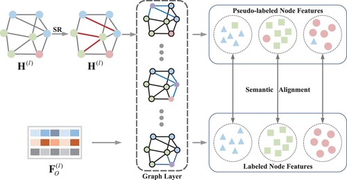
4.1. Structural reinforcement

Like SelfSAGCN Yang et al. (2021), SRGCN also adopts two perspectives with different inputs. The first perspective is graph aggregation, i.e. feature aggregation and propagation using the feature matrix $\mathit{X}$ and the adjacency matrix $\mathit{A}$. It can be described as: (4) $\begin{array}{rl}& {\mathit{H}}^{(0)}=\mathit{X}\\ & {\mathit{H}}^{(l+1)}=\sigma \left(\tilde{\mathit{P}}{\mathit{H}}^{(l)}{\mathit{W}}^{(l)}\right)(l=0,1,2,\dots ,L-1)\end{array}$(4) The second perspective is feature aggregation, which is the aggregation and propagation of features with feature matrix $\mathit{X}$ only. It can be described as: (5) $\begin{array}{rl}& {\mathit{F}}^{(0)}=\mathit{X}\\ & {\mathit{F}}^{(l+1)}=\sigma \left(\mathit{I}{\mathit{F}}^{(l)}{\mathit{W}}^{(l)}\right)(l=0,1,2,\dots ,L-1)\end{array}$(5) After aggregation in both perspectives, we extract the structural semantics by the phase subtraction operation. In addition, the structural semantics is added to the graph semantics to enhance the feature propagation capability: (6) ${\mathit{H}}^{(l)}\leftarrow {\mathit{H}}^{(l)}+\beta ({\mathit{H}}^{(l)}-{\mathit{F}}_O^{(l)})$(6) where β represents the balance parameter and ${\mathit{F}}_O^{(l)}$ indicates the semantics learned from labeled nodes. The final output is ${\mathit{H}}^{\mathrm{out}}=\mathrm{softmax}({\mathit{H}}^{(L)})\in {\mathbb{R}}^{n\times c}$ and ${\mathit{F}}^{\mathrm{out}}=\mathrm{softmax}({\mathit{F}}^{(L)})\in {\mathbb{R}}^{n\times c}$. Finally, the model's loss function is defined with cross-entropy and can be described as: (7) $Los{s}_{semi}=-\sum _{i\in O}\sum _{k=1}^c({\mathit{Y}}_{ik}\ln {\mathit{H}}_{ik}^{out}+{\mathit{Y}}_{ik}\ln {\mathit{F}}_{ik}^{out})$(7) where O is the set of labeled nodes.

In addition, Li et al. (2018) demonstrated that a multiple layers model of GCN makes the features of nodes become the same value. Specifically, each node's higher-order relations contain many identical neighbors in a network with denser edges. The more repetitive information aggregated in the node features results in a poorer representation of the generated nodes as the propagation range expands. Therefore, the last item of $Los{s}_{semi}$ is employed to provide discriminative information for feature propagation in the graph from the feature perspective.

4.2. Semantic alignment

According to the propagation rules, we can find that the parameters of ${\mathit{F}}^{(l)}$ and ${\mathit{H}}^{(l)}$ are the same. ${\mathit{F}}^{(l)}$ denotes feature propagation, so the value of subtraction (${\mathit{H}}^{(l)}-{\mathit{F}}_O^{(l)}$) represents the influence of the structure in the graph propagation process. Adding the value back to ${\mathit{H}}^{(l)}$ represents our expectation of strengthening the influence of structure in the propagation process. Notably, ${\mathit{F}}^{(l)}$ does not have the problem of over-smoothing and can be treated as a constraint in the ${\mathit{H}}^{(l)}$ propagation process. In addition, we utilize semantic alignment techniques to make ${\mathit{F}}_O^{(l)}$ and ${\mathit{H}}^{(l)}$ semantically similar, which enables unlabeled nodes to draw inspiration from labeled nodes.

During model training, the semantic alignment of nodes can be handled in two cases. The first case is labeled nodes, i.e. ${\mathit{F}}_O^{(l)}$ and labeled nodes in the ${\mathit{H}}^{(l)}$ can directly adopt the labels as the class. The second case is the unlabeled nodes in the ${\mathit{H}}^{(l)}$, for which we need to assign pseudo-labels and use class-centered similarity to mitigate the effect of noise in the assignment process. A class-centered similarity of the single layer can be described as: (8) $Los{s}_{sema}=\sum _{j=1}^c\mathrm{sed}({\mathit{C}}_j\left({\mathit{F}}_O^{(l)}\right),{\mathit{C}}_j\left({\mathit{H}}^{(l)}\right))$(8) where ${\mathit{C}}_j({\mathit{F}}_O^{(l)})$ and ${\mathit{C}}_j({\mathit{H}}^{(l)})$ are the $j^{th}$ class-centered of ${\mathit{F}}_O^{(l)}$ and ${\mathit{H}}^{(l)}$, respectively. In addition, $\mathrm{sed}(\cdot )$ denotes the function that calculates the squared Euclidean distance.

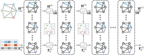
The structure of SRGCN is displayed in Figure 2. The model extracts semantics layer by layer and exploits feature propagation to guide graph propagation while reinforcing the structure. With this method, the over-smoothing and over-fitting problems can be alleviated. In addition, the class-centered similarity can provide extra supervised information for classification learning tasks. The model's class-centered similarity can be described as: (9) $Los{s}_{sema}=\sum _{l=1}^L\sum _{j=1}^c\mathrm{sed}({\mathit{C}}_j\left({\mathit{F}}_O^{(l)}\right),{\mathit{C}}_j\left({\mathit{H}}^{(l)}\right))$(9) Combining the two loss components, we can describe the total objective function as: (10) $Loss=Los{s}_{semi}+\lambda \cdot Los{s}_{sema}$(10) In addition, to ensure the stability of the class-centered, we utilize the previous class-centered to accumulate with the weighted class-centered of the current layer during the iteration: (11) $\begin{array}{rl}{\mathit{C}}_j^t\left({\mathit{F}}_O^{(l)}\right)& \leftarrow (1-\alpha ){\mathit{C}}_j^t\left({\mathit{F}}_O^{(l)}\right)+\alpha {\mathit{C}}_j^{(t-1)}\left({\mathit{F}}_O^{(l)}\right)\\ {\mathit{C}}_j^t\left({\mathit{H}}^{(l)}\right)& \leftarrow (1-\alpha ){\mathit{C}}_j^t\left({\mathit{H}}^{(l)}\right)+\alpha {\mathit{C}}_j^{(t-1)}\left({\mathit{H}}^{(l)}\right)\end{array}$(11) where ${\mathit{C}}_j^t(\cdot )$ and ${\mathit{C}}_{j-1}^t(\cdot )$ denote the class-centered of the $(m-1{)}^{th}$ and $m^{th}$ layers, respectively. $\alpha \in [0,1)$ indicates the weighting factor.

Figure 2. The overall structure of SRGCN. We first extract the semantics layer by layer from both graph and feature perspectives, reinforce the structural influence in graph propagation, and then use semantic alignment to align the processed semantic information.

4.3. Further analysis

It is assumed that neighbors have the same label, so graph propagation can pass features from labeled to unlabeled nodes with graph structure. However, Liu et al. (2020) proved that the core of label determination is the features of the node rather than the topology so that we can identify the node's label by its features in the ideal environment. Yang et al. (2021) extracted semantics from both graph and feature perspectives and employed feature semantics to assist the feature propagation process in the graph. Qin et al. (2022) extracted semantics from three perspectives: graph, features, and nodes, and reinforced the same parts of the semantics to constrain the graph propagation process. Based on the previous work summary, we strengthen the information of the structure in the graph and improve the features propagation from both the graph and feature perspectives. The model mitigates over-smoothing and over-fitting problems by reinforcing structural semantics in the graph propagation process and using feature propagation aids.

In addition, we exploit the semantic alignment operation to force the obtained semantic distributions to converge, making the graph propagation process constrained by the feature propagation. The class-centered similarity can also enable unlabeled nodes to gain inspiration from the learning process of labeled nodes. In summary, structural reinforcement and feature propagation can provide additional supervisory information for graph propagation. It is worth noting that the objective function of SRGCN looks more complex than that of GCN, but the time complexity of both is $O(|E|DHF)$, where E denotes the number of edges in the graph, D indicates the dimension of the input nodes, H represents the dimension of the hidden layer, and F is the dimension of the output layer.

5. Experiments

We conduct extensive experiments on three standard datasets for evaluating the performance of SRGCN in this section. In addition, we will offer some visualizations to assist in illustrating the experimental effects.

5.1. Datasets and baseline

We conduct model testing on three standard datasets: Cora McCallum et al. (2000); Yang et al. (2021), Citeseer Giles et al. (1998); Yang et al. (2021), and Pubmed Sen et al. (2008); Yang et al. (2021). The dataset's nodes, labels, and edges represent the papers, topics, and reference associations. The features of nodes are the bag of words. A brief description of the three datasets is as follows:

• Cora has a total of 2708 nodes with 1433-dimensional features, 7 classes of node labels, and 5420 edges between nodes.

• Citeseer has a total of 3327 nodes with 3707-dimensional features, 6 classes of node labels, and 4732 edges between nodes.

• Pubmed has a total of 19717 nodes with 400-dimensional features, 3 classes of node labels, and 44338 edges between nodes.

In addition, we mainly perform model performance comparisons under two scenarios, so we divide the baseline methods into two groups.

• Labeled nodes are severely limited: GCN Kipf and Welling (2016), SGC Wu et al. (2019), GAT Veličković et al. (2017), APPNP Klicpera et al. (2018), ICGN Li et al. (2019), DAGNN Liu et al. (2020), Shoestring Lin et al. (2020), SelfSAGCN Yang et al. (2021), MSAGCN Qin et al. (2022).

• The model is multi-layer: DropEdge Rong et al. (2019), ResGCN Li et al. (2019), IncepGCN Rong et al. (2019), GCNII Chen et al. (2020), JKNet Xu et al. (2018), SelfSAGCN Yang et al. (2021), MSAGCN Qin et al. (2022).

5.2. Setup

The SRGCN is implemented with Pytorch¹ and adopts the code of SelfSAGCN Yang et al. (2021)². In addition, to facilitate a fair comparison with the baseline methods, we try to keep our parameters consistent with those of GCN Kipf and Welling (2016). Specifically, we employ the Adam optimizer Kingma and Ba (2014), and the learning rate, dropout, and weight decay are set to 0.01, 0.5, and 5e−4, respectively. The class-centered factor α is set to 0.7 and the reinforcement coefficient β of structural semantics is set to 0.25. To suppress the noise of the pseudo-labels, λ ($\lambda \leftarrow \lambda (\frac{2}{1+e^{-10\times p}}-1)$) is utilised early in training. In the deep model, the number of graph propagation layers equals the number of hidden layers. In addition, to ensure fairness, the obtained experimental data are averaged after 20 experiments.

5.3. Performance comparison

We evaluated the performance of SRGCN when it contains 20 labeled nodes in each class, and the result is shown in Table 1. It shows that SRGCN can obtain relatively excellent performance.

Table 1. Performance comparison of models with 20 labeled nodes in each class (%).

Method	Cora	Pubmed	Citeseer
MLP	61.6 ± 0.2	74.2 ± 0.2	61.0 ± 0.3
GCN	81.2 ± 0.4	78.5 ± 1.0	71.1 ± 0.7
SGC	81.7 ± 0.6	78.9 ± 1.3	71.3 ± 1.1
Shoestring	81.9 ± 2.1	79.7 ± 4.5	69.5 ± 2.4
GAT	83.1 ± 0.7	71.1 ± 1.2	70.8 ± 0.9
APPNP	83.3 ± 2.4	80.1 ± 1.3	71.8 ± 0.9
SelfSAGCN	83.8 ± 0.5	80.7 ± 1.5	73.5 ± 1.2
MSAGCN	84.0 ± 0.6	80.5 ± 1.2	73.8 ± 0.9
DAGNN	84.4 ± 0.4	80.5 ± 0.9	73.3 ± 0.7
SRGCN	84.3 ± 0.5	80.9 ± 1.1	73.8 ± 1.5

5.4. Model performance with severely limited labeled nodes

We evaluate the performance of SRGCN when labeled nodes are severely limited. Table 2 shows the performance of SRGCN and baseline methods when the number of labeled nodes in each class is 1, 2, and 5.

Table 2. Model performance when labeled nodes are severely limited (%).

	1 label			2 labels			5 labels
Method	Cora	Pubmed	Citeseer	Cora	Pubmed	Citeseer	Cora	Pubmed	Citeseer
GCN	43.1 ± 0.7	51.5 ± 1.8	29.2 ± 0.9	58.0 ± 0.6	60.4 ± 2.3	40.5 ± 0.7	69.1 ± 0.5	68.4 ± 3.2	53.7 ± 0.9
GAT	45.2 ± 0.6	53.5 ± 2.3	32.5 ± 1.0	59.7 ± 0.4	62.2 ± 2.2	43.2 ± 0.7	70.2 ± 0.3	69.5 ± 1.1	55.2 ± 0.7
APPNP	45.2 ± 0.3	52.3 ± 3.2	33.5 ± 1.2	58.3 ± 0.7	62.7 ± 1.3	50.1 ± 0.6	71.2 ± 0.5	70.7 ± 1.3	55.9 ± 0.9
SGC	44.5 ± 0.5	55.2 ± 2.3	31.4 ± 0.9	58.6 ± 0.5	63.5 ± 2.9	45.8 ± 0.6	69.5 ± 0.4	71.4 ± 2.9	54.6 ± 0.8
ICGN	43.3 ± 0.5	54.2 ± 1.5	35.0 ± 1.1	63.5 ± 2.7	62.6 ± 3.2	43.9 ± 1.9	72.2 ± 2.5	70.7 ± 1.3	55.9 ± 0.9
DAGNN	59.2 ± 0.4	58.5 ± 2.4	45.2 ± 0.7	65.6 ± 0.8	65.3 ± 2.7	54.3 ± 0.8	72.0 ± 0.4	71.4 ± 2.2	58.1 ± 0.9
Shoestring	60.2 ± 0.9	60.3 ± 6.1	52.2 ± 1.3	68.3 ± 0.9	63.5 ± 5.7	60.1 ± 1.3	73.0 ± 1.2	68.4 ± 6.3	64.2 ± 1.5
SelfSAGCN	63.5 ± 0.8	65.0 ± 3.3	57.5 ± 3.7	71.7 ± 0.6	70.9 ± 1.9	68.3 ± 1.2	75.1 ± 0.7	73.0 ± 2.1	71.9 ± 1.3
MSAGCN	65.2 ± 0.7	67.7 ± 2.2	60.1 ± 2.1	73.1 ± 0.5	70.7 ± 1.7	69.5 ± 1.7	77.4 ± 0.5	72.8 ± 1.6	72.8 ± 1.1
SRGCN	67.6 ± 0.7	68.9 ± 2.5	60.3 ± 2.9	74.3 ± 0.7	71.1 ± 1.5	69.5 ± 1.4	77.6 ± 0.7	73.5 ± 1.9	72.7 ± 1.3

The following conclusions can be drawn from Table 2:

• SRGCN achieves competitive performance when labeled nodes are severely limited. It illustrates that strengthening the structural messages in the graph propagation process can enhance the propagation of features and alleviate the over-fitting problem.

• The model performs better when the number of labeled nodes is severely limited. In addition, the advantage of the model becomes weak as the number of labeled nodes increases, indicating that the advantage of reinforcing structural information acquisition becomes weak.

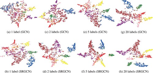
To help illustrate, we visualise the distribution of node features in Figure 3 when various numbers of labeled nodes are present on the Cora dataset with t-SNE Van der Maaten and Hinton (2008), where the same color means that the nodes belong to the same class.

Figure 3. Visualize the distribution of nodes on the Cora dataset. The number of labeled nodes is 1, 2, 5, 20. (a) 1 label (GCN) (b) 1 label (SRGCN) (c) 2 labels (GCN) (d) 2 labels (SRGCN) (e) 5 labels (GCN) (f) 5 labels (SRGCN) (e) 20 labels (GCN) (f) 20 labels (SRGCN).

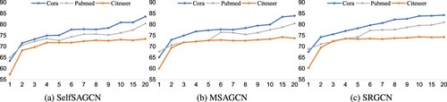
In addition, we evaluate the performance of three models with various numbers of labeled nodes, including SelfSAGCN Yang et al. (2021), MSAGCN Qin et al. (2022), and SRGCN, and the results are shown in Figure 4.

Figure 4. The performance of the three models with various numbers of labeled nodes. (a) SelfSAGCN (b) MSAGCN (c) SRGCN.

The following conclusions can be drawn from Table 4:

• For Cora and Pubmed, the performance of the three models increases with the number of labeled nodes. In addition, the SRGCN has the fastest performance improvement.

• For the Citeseer, the three models perform similarly. The performance increases dramatically when the number of labeled nodes is increased from 1 to 2. When the number of labeled nodes is increased from 2 to 20, there is almost no increase in performance.

5.5. Parameter analysis

This section analyzes the effects of different parameters in SRGCN on the model's performance, and the results are shown in Figure 5.

Figure 5. Effect of different hyperparameters on model performance on the Cora dataset. (a) The reinforcement coefficient β of structural semantics. (b) The balance weight λ in the objective loss function. (c) The balance coefficient α in class-centered alignment.

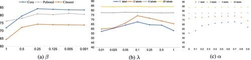
From Figure 5, we can obtain the following conclusions:

• As shown in Figure 5(a), when the number of labeled nodes is severely limited, the change in the value of the reinforcement coefficient for structural semantics significantly impacts the model performance. However, when the number of labeled nodes increases, the model's sensitivity to the reinforcement coefficient decreases. The reason is that when the labeled nodes are severely limited, the enhanced structural semantics can improve the graph's propagation of features.

• As shown in Figure 5(b), when λ is appropriate, semantic alignment works well to provide additional supervisory information for graph propagation. Furthermore, when $\lambda \in [0.1,0.5]$, the model's performance is insensitive to its value.

• From Figure 5(c), it is evident that class-centered similarity optimisation can help the model's training process to suppress the noise problem caused by pseudo-labels. In addition, when α is too big, the class-centered construction obtains less class-centered data from the current layer and too much from the upper layer, resulting in poor performance of the model.

• As shown in Figure 5(b-c), the model's sensitivity to the parameters decreases when the number of labeled nodes increases.

5.6. Performance of multiple layer models

We evaluate the performance of SRGCN and the baseline models in the case of multiple layers of structure, and the result is shown in Table 3. As in the previous work, 20 labeled nodes in each class are involved in model training.

Table 3. Performance of the model under multiple layers structure (%).

	4 Layers			8 Layers			16 Layers
Method	Cora	Pubmed	Citeseer	Cora	Pubmed	Citeseer	Cora	Pubmed	Citeseer
GCN	80.4 ± 0.4	79.0 ± 1.2	67.6 ± 0.9	69.5 ± 0.1	61.2 ± 1.5	30.2 ± 0.3	64.9 ± 1.4	40.9 ± 0.7	18.3 ± 1.1
GCNdrop	82.0 ± 0.7	79.1 ± 1.4	70.2 ± 0.8	75.8 ± 0.4	78.1 ± 0.7	61.4 ± 0.5	75.7 ± 1.1	78.5 ± 1.5	57.2 ± 0.9
JKNet	80.2 ± 0.5	78.0 ± 1.0	68.7 ± 0.4	80.7 ± 0.6	78.1 ± 1.4	67.7 ± 0.3	80.2 ± 1.0	72.6 ± 1.4	69.8 ± 0.7
IncepGCN	77.6 ± 0.5	77.0 ± 0.7	69.3 ± 0.6	76.5 ± 0.8	77.9 ± 1.2	68.4 ± 0.5	81.7 ± 0.7	74.9 ± 1.7	70.2 ± 0.9
ResGCN	78.8 ± 0.6	78.6 ± 1.5	70.5 ± 0.6	75.6 ± 0.5	78.1 ± 1.3	65.0 ± 0.4	72.0 ± 0.8	75.5 ± 1.0	66.5 ± 0.5
DAGNN	82.1 ± 0.5	77.5 ± 0.9	68.5 ± 0.9	83.2 ± 0.6	78.4 ± 0.9	70.2 ± 0.4	81.7 ± 0.8	79.8 ± 1.0	68.4 ± 0.9
SelfSAGCN	82.3 ± 0.3	79.5 ± 1.2	72.3 ± 0.8	81.9 ± 0.5	78.7 ± 1.3	71.0 ± 1.1	80.5 ± 0.3	78.1 ± 1.4	68.0 ± 1.2
MSAGCN	83.0 ± 0.6	79.3 ± 0.9	72.3 ± 0.6	82.4 ± 0.7	78.0 ± 1.5	71.3 ± 0.8	82.1 ± 0.5	77.3 ± 1.3	68.9 ± 0.9
GCNII	82.0 ± 0.4	78.6 ± 0.4	68.7 ± 0.4	84.1 ± 0.3	79.4 ± 0.6	70.6 ± 0.5	84.6 ± 0.8	80.2 ± 1.0	72.9 ± 0.9
SRGCN	83.3 ± 0.5	79.7 ± 1.0	72.5 ± 0.5	83.0 ± 0.7	79.0 ± 0.9	71.6 ± 0.6	81.7 ± 1.1	78.9 ± 1.3	68.3 ± 1.0

As shown in Table 3, SRGCN can still obtain good performance at 4 layers. It indicates that the enhanced structural semantics in the graph propagation process can relieve the over-smoothing problem.

6. Conclusion

To alleviate the over-fitting and over-smoothing problems of GCN, we propose a structural reinforcement-based graph convolutional network (SRGCN) that contains two essential techniques: structural reinforcement and semantic alignment. Specifically, the model extracts semantic information and reinforces structural semantics in the graph layer by layer from both graph and feature perspectives. The semantic alignment operation is then employed to align the two parts of the semantic information, providing additional supervision conditions for graph propagation. This method can effectively mitigate the problem of over-fitting and over-smoothing due to poor propagation of features. In addition, the class-centered alignment can effectively alleviate the noise problem caused by pseudo-labels, allowing unlabeled nodes to be inspired by labeled nodes. The experimental results on three citation datasets demonstrate that SRGCN can achieve excellent performance. The proposal of SRGCN has promoted the development and application of network topology optimisation and structural reinforcement research. In the future, we will investigate how to enhance the propagation of features in directed graphs.

Disclosure statement

No potential conflict of interest was reported by the author(s).

Additional information

Funding

This work was supported by the Postgraduate Research & Practice Innovation Program of Jiangsu Province.

Notes

1 https://pytorch.org

2 https://github.com/xdxuyang/SelfSAGCN

References

- Atwood, J., & Towsley, D. (2016). Diffusion-convolutional neural networks. In Advances in neural information processing systems (p. 29). Curran Associates, Inc.
- Bian, T., Xiao, X., Xu, T., Zhao, P., Huang, W., Rong, Y., & Huang, J. (2020). Rumor detection on social media with bi-directional graph convolutional networks. In Proceedings of the AAAI conference on artificial intelligence (Vol. 34, No. 01, pp. 549–556). AAAI Press. https://doi.org/10.1609/aaai.v34i01.5393.
- Bruna, J., Zaremba, W., Szlam, A., & LeCun, Y. (2013). Spectral networks and locally connected networks on graphs. arXiv preprint arXiv:1312.6203.
- Chen, G., & Zhang, J. (2022). Preventing over-smoothing for hypergraph neural networks. arXiv preprint arXiv:2203.17159.
- Chen, M., Wei, Z., Huang, Z., Ding, B., & Li, Y. (2020). Simple and deep graph convolutional networks. In International conference on machine learning (pp. 1725–1735). PMLR.
- Defferrard, M., Bresson, X., & Vandergheynst, P. (2016). Convolutional neural networks on graphs with fast localized spectral filtering. In Advances in neural information processing systems (p. 29). Curran Associates, Inc.
- Donnat, C., Zitnik, M., Hallac, D., & Leskovec, J. (2018). Learning structural node embeddings via diffusion wavelets. In Proceedings of the 24th ACM SIGKDD international conference on knowledge discovery & data mining (pp. 1320–1329). Association for Computing Machinery. https://doi.org/10.1145/3219819.3220025.
- Feng, F., He, X., Zhang, H., & Chua, T. S. (2021). Cross-GCN: enhancing graph convolutional network with k-order feature interactions. IEEE Transactions on Knowledge and Data Engineering. https://doi.org/10.1109/TKDE.2021.3077524.
- Giles, C. L., Bollacker, K. D., & Lawrence, S. (1998). CiteSeer: an automatic citation indexing system. In Proceedings of the third ACM conference on digital libraries (pp. 89–98). Association for Computing Machinery.
- Gilmer, J., Schoenholz, S. S., Riley, P. F., Vinyals, O., & Dahl, G. E. (2017). Neural message passing for quantum chemistry. In International conference on machine learning (pp. 1263–1272). PMLR.
- Hamilton, W., Ying, Z., & Leskovec, J. (2017). Inductive representation learning on large graphs. In Advances in neural information processing systems (p. 30). Curran Associates, Inc.
- Hu, J., Guo, C., Yang, B., & Jensen, C. S. (2019). Stochastic weight completion for road networks using graph convolutional networks. In 2019 IEEE 35th international conference on data engineering (ICDE) (pp. 1274–1285). IEEE. https://doi.org/10.1109/ICDE.2019.00116.
- Jo, J., Baek, J., Lee, S., Kim, D., Kang, M., & Hwang, S. J. (2021). Edge representation learning with hypergraphs. Advances in Neural Information Processing Systems, 34, 7534–7546.
- Kingma, D. P., & Ba, J. (2014). Adam: a method for stochastic optimisation. arXiv preprint arXiv:1412.6980.
- Kipf, T. N., & Welling, M. (2016). Semi-supervised classification with graph convolutional networks. arXiv preprint arXiv:1609.02907.
- Klicpera, J., Bojchevski, A., & Günnemann, S. (2018). Predict then propagate: graph neural networks meet personalised pagerank. arXiv preprint arXiv:1810.05997.
- Klicpera, J., Weißenberger, S., & Günnemann, S. (2019). Diffusion improves graph learning. arXiv preprint arXiv:1911.05485.
- Li, G., Muller, M., Thabet, A., & Ghanem, B. (2019). Deepgcns: can gcns go as deep as cnns? In Proceedings of the IEEE/CVF international conference on computer vision (pp. 9267–9276). IEEE.
- Li, Q., Han, Z., & Wu, X. M. (2018). Deeper insights into graph convolutional networks for semi-supervised learning. In Thirty-Second AAAI conference on artificial intelligence. AAAI Press.
- Li, Q., Wu, X. M., Liu, H., Zhang, X., & Guan, Z. (2019). Label efficient semi-supervised learning via graph filtering. In Proceedings of the IEEE/CVF conference on computer vision and pattern recognition (pp. 9582–9591). IEEE.
- Lin, W., Gao, Z., & Li, B. (2020). Shoestring: graph-based semi-supervised classification with severely limited labeled data. In Proceedings of the IEEE/CVF conference on computer vision and pattern recognition (pp. 4174–4182). IEEE.
- Liu, M., Gao, H., & Ji, S. (2020). Towards deeper graph neural networks. In Proceedings of the 26th ACM SIGKDD international conference on knowledge discovery & data mining (pp. 338–348). Association for Computing Machinery. https://doi.org/10.1145/3394486.3403076.
- Liu, M., Wang, Z., & Ji, S. (2021). Non-local graph neural networks. IEEE Transactions on Pattern Analysis and Machine Intelligence, 44(12), 10270–10276. https://doi.org/10.1109/TPAMI.2021.3134200
- McCallum, A. K., Nigam, K., Rennie, J., & Seymore, K. (2000). Automating the construction of internet portals with machine learning. Information Retrieval, 3(2), 127–163. https://doi.org/10.1023/A:1009953814988
- Mishra, P., Del Tredici, M., Yannakoudakis, H., & Shutova, E. (2019). Abusive language detection with graph convolutional networks. arXiv preprint arXiv:1904.04073. https://doi.org/10.48550/arXiv.1904.04073.
- Monti, F., Boscaini, D., Masci, J., Rodola, E., Svoboda, J., & Bronstein, M. M. (2017). Geometric deep learning on graphs and manifolds using mixture model cnns. In Proceedings of the IEEE conference on computer vision and pattern recognition (pp. 5115–5124). IEEE.
- Pei, H., Wei, B., Chang, K. C. C., Lei, Y., & Yang, B. (2020). Geom-gcn: geometric graph convolutional networks. arXiv preprint arXiv:2002.05287.
- Qin, J., Zeng, X., Wu, S., & Tang, E. (2021). E-GCN: graph convolution with estimated labels. Applied Intelligence, 51(7), 5007–5015. https://doi.org/10.1007/s10489-020-02093-5
- Qin, J., Zeng, X., Wu, S., & Zou, Y. (2022). Feature recommendation strategy for graph convolutional network. Connection Science, 34(1), 1697–1718. https://doi.org/10.1080/09540091.2022.2080806
- Qin, J., Zeng, X., Wu, S., & Zou, Y. (2022). Multi-Semantic Alignment Graph Convolutional Network. Connection Science, 34(1), 2313–2331. https://doi.org/10.1080/09540091.2022.2115010
- Rong, Y., Huang, W., Xu, T., & Huang, J. (2019). Dropedge: towards deep graph convolutional networks on node classification. arXiv preprint arXiv:1907.10903.
- Sen, P., Namata, G., Bilgic, M., Getoor, L., Galligher, B., & Eliassi-Rad, T. (2008). Collective classification in network data. AI Magazine, 29(3), 93–93. https://doi.org/10.1609/aimag.v29i3.2157
- Shang, C., Tang, Y., Huang, J., Bi, J., He, X., & Zhou, B. (2019). End-to-end structure-aware convolutional networks for knowledge base completion. In Proceedings of the AAAI conference on artificial intelligence (Vol. 33, No. 01, pp. 3060–3067). AAAI Press. https://doi.org/10.1609/aaai.v33i01.33013060.
- Tan, Z., Yang, Y., Wan, J., Guo, G., & Li, S. Z. (2020). Relation-aware pedestrian attribute recognition with graph convolutional networks. In Proceedings of the AAAI conference on artificial intelligence (Vol. 34, pp. 12055–12062). AAAI Press. https://doi.org/10.1609/aaai.v34i07.6883.
- Van der Maaten, L., & Hinton, G. (2008). Visualizing data using t-SNE. Journal of Machine Learning Research, 9(11), 2579–2605.
- Veličković, P., Cucurull, G., Casanova, A., Romero, A., Lio, P., & Bengio, Y. (2017). Graph attention networks. arXiv preprint arXiv:1710.10903.
- Wu, F., Souza, A., Zhang, T., Fifty, C., Yu, T., & Weinberger, K. (2019). Simplifying graph convolutional networks. In International conference on machine learning (pp. 6861–6871). PMLR.
- Xia, L., Huang, C., Xu, Y., Zhao, J., Yin, D., & Huang, J. (2022). Hypergraph contrastive collaborative filtering. In Proceedings of the 45th International ACM SIGIR conference on research and development in information retrieval (pp. 70–79). https://doi.org/10.1145/3477495.3532058.
- Xu, K., Li, C., Tian, Y., Sonobe, T., Kawarabayashi, K. I., & Jegelka, S. (2018). Representation learning on graphs with jumping knowledge networks. In International conference on machine learning (pp. 5453–5462). PMLR.
- Xu, K., Li, J., Zhang, M., Du, S. S., Kawarabayashi, K. I., & Jegelka, S. (2019). What can neural networks reason about? arXiv preprint arXiv:1905.13211.
- Yang, L., Kang, Z., Cao, X., Jin, D., Yang, B., & Guo, Y. (2019). Topology optimisation based graph convolutional network. In IJCAI (pp. 4054–4061). AAAI Press.
- Yang, X., Deng, C., Dang, Z., Wei, K., & Yan, J. (2021). SelfSAGCN: self-supervised semantic alignment for graph convolution network. In Proceedings of the IEEE/CVF conference on computer vision and pattern recognition (pp. 16775–16784). IEEE.
- Zhang, J., Shi, X., Xie, J., Ma, H., King, I., & Yeung, D. Y. (2018). Gaan: gated attention networks for learning on large and spatiotemporal graphs. arXiv preprint arXiv:1803.07294.