Assessment of interferometric coherence contribution to corn and soybean mapping with Sentinel-1 data time series

Abstract

This work aims to evaluate the added value of interferometric coherence to backscatter information of Synthetic Aperture Radar (SAR) systems for soybean and corn mapping. First, SAR response to crop growth, and then accuracies for the classification using a combination of SAR variables were evaluated for scenarios that employ in-season or the entire season time series. Results showed that: i) using a single feature, the backscatter at vertical-horizontal (VH) polarization would be the most suitable variable; ii) the complementarity of coherence to single backscatter at vertical-vertical (VV) polarization was demonstrated, adding a significant contribution to late sown corns differentiation and iii) the combination of VV and VH backscatter would be the preferable variables for the proposed classification. In this case, the adding of coherence did not show a significant accuracy improvement, while a high computational cost is required. Finally, high general accuracies (until 90%) for early-season maps were achieved.

Keywords:

• InSAR coherence
• crop mapping
• SAR time series

1. Introduction

Soybean (Glycine max L.) and corn (Zea mays L.) are two of the most important food crops in the world. They are extensively grown all over the globe and attract considerable attention in global food production. Maize is a high-yield crop with extremely high nutritional value, and soybean is an important high-protein raw material for food production. Therefore, these crops are of great importance for national food security in many countries (She et al. 2020). In this context, Argentina has been the fourth main corn producer (third exporter), and the third one for soybean in the last 5 years (FAO 2022). In 2021, the sowed area of soybean in Argentina reached 16.7 MH, and the acreage of corn reached 7.7 MH (Di Yenno and Terré 2021). Having a spring-summer-autumn cycle, these crops compete with each other. Then, the identification of these crops is relevant for agricultural systems, providing basic information for regional crop growth conditions and yield estimates (Aoki et al. 2021). In this sense, crop rotations are key agronomic tools to enhance farm productivity, preserve the soil, and ensure provision of ecosystem services (J. Li et al. 2019; Bowles et al. 2020). The knowledge of the spatio-temporal distribution of crops is essential to characterize rotations at field scale and estimate their impacts on several outcomes (Aoki et al. 2021). In this context, crop mapping at field scale is the first step and a key point to monitor agricultural systems. This allows public policymakers and private managers obtaining valuable information related to food production and sustainability, logistic planning, supply chain evaluation for other industries, research priorities identification, and commodity markets evaluation, among others (Pott et al. 2021).

Remote sensing has widely proven to be a reliable tool for crop mapping purposes. Satellite data provide a timely, efficient, low-cost, and objective tool to crop identification and mapping at large-scale (Weiss et al. 2020). Among remote sensing data, optical images have been the most used satellite imagery for cropland mapping. Moreover, Synthetic Aperture Radar (SAR) data has demonstrated to provide complementary information to optical data for crop classification purposes (Blaes et al. 2005; McNairn et al. 2009). SAR is an active microwave remote sensing technique. Being independent of external light sources and atmospheric condition, it can continuously collect data. This characteristic avoids missing information due to cloudy or rainy weather during crop growing season, which is the main problem for optical imaging systems (L. Li et al. 2019). Also, scattering response of SAR systems signal is strongly linked to the crop canopy along crop life cycle due to the signal sensitivity to geometric and moisture conditions (McNairn et al. 2014).

The use of optical remote sensing to map the corn and soybean distribution has been confirmed worldwide (Chang et al. 2007; Zhong et al. 2016; Cai et al. 2018; Wang et al. 2019; Wang et al. 2020). Furthermore, previous works have evaluated the use of SAR imagery time series (McNairn et al. 2014; Whelen and Siqueira 2018; Dingle Robertson et al. 2020; Amherdt et al. 2021), as well as the synergy of SAR and optical data (Pott et al. 2021) for corn and soybean mapping. However, such classification is not usually estimated at an early stage of the crops growing season, which is important to assist with production forecasts (McNairn et al. 2014). For crop mapping, both intensity and polarimetric variables are the most used among SAR information (McNairn and Shang 2016). On the other hand, phase information is not frequently exploited for such purposes. Recently, Busquier et al. (2020) and Mestre-Quereda et al. (2020) evaluated SAR coherence for crop-type mapping in Sevilla, Spain, whose results suggest the complementarity of coherence to backscatter information.

Therefore, in the present study time series of backscatter at vertical transmitted-vertical received (VV) and vertical transmitted-horizontal received (VH) polarization, as well as coherence information from C-band SAR images acquired by the Sentinel-1 satellites were used aiming to:

1. Assess the contribution of interferometric coherence to backscatter information for soybean and corn mapping, discerning crop sequences, as well as early and late sown crops.

2. Evaluate the contribution of SAR data for periods linked to corns and soybeans growth stages for their mapping, as well as the in-season maps accuracies.

2. Materials and methods

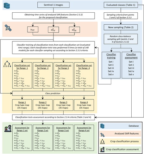
The general scheme for proposed classifications in this work is depicted in Figure 1.

Figure 1. Study workflow.

2.1. Study area

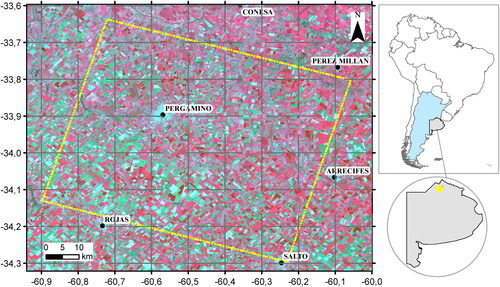
The study area is located in the core agricultural region of Argentina, in the northern of Buenos Aires province. This area is included in the sub-region of the Undulated Pampa, within the Humid Pampa region. The study area covers a total of 366620 hectares and lies between 33° 33′ 13'' and 34° 17′ 47'' south latitude and 60° 03′ 27'' and 60° 53′ 51'' west longitude (Figure 2). Climate typeof the region is humid/subhumid, with average annual rainfall of 1056 mm. Fall and spring/summer are rainy seasons, with a considerable variability in monthly and annual precipitations. Soils of the study area were developed from loess-like sediments and are mainly Mollisols.

Figure 2. On the right side, in yellow, the study area location in the north of Buenos Aires province. On the left side, study area extension represented by the yellow rectangle (background: ‘color-infrared’ composite from Landsat-9 images acquired on March 27, 2022).

Extensive cereal and oil crops are produced under rainfed conditions and with no-tillage cropping system. The main one in the study area is soybean, which covers around 75% of summer field crop acreage (Bitar et al. 2020). On a year basis, soybean is cropped as a single crop (full season soybean) or in a wheat/soybean sequence (hereafter named WC-Soybean). In this case, despite the lower soybean yield due to its seeding time after the optimal period, the farm income is higher due to the double harvest in the year. On the other hand, corn is the second summer crop most widely sowed in the region with 19% of the cropped area (Bitar et al. 2020). Sowing period of maize is distributed between early (September–early October) and late (end of November–December) (Gayo and López 2018). Within the late planted, a small proportion of fields follow a winter crop (wheat, barley, winter legumes, among others), hereinafter called WC-Corn, while most of fields are preceded by a fallow period much longer than early sowing. (Late Corn). For the late sown corn, a better fit of rainfall supply and the crop evapotranspirative demand is achieved due to the less demanding atmospheric conditions in March and April (Otegui et al. 2021). Due to this, between 15 and 25% of the total sown area corresponds to late-sown corn (both single crop or a crop sequence), according to previous estimates (Gayo and López 2018).

For crop sequences (both WC-Soybean and WC-Corn), winter crops are usually harvested during the months of November and December.

2.2. Data

2.2.1. SAR data

In this study, 49 Sentinel-1 single look complex (SLC) images were available for the studied period from 2019-10-14 to 2020-08-21. Data was obtained from the Copernicus Open Access Hub (https://scihub.copernicus.eu/) server. Employed images were acquired in Interferometric Wide Swath (IW) mode every 6 days for most of the period (except in 4 cases, with a temporal difference of 12 days) depending on data availability. Images at IW mode have a nominal spatial resolution of 20 by 5 meters in azimuth and range direction, respectively, and a Maximum Noise Equivalent Sigma Zero of −22 dB (Attema et al. 2010). Further, only a single sub-swath (IW3) of the images in descending orbit (number 68) were used. Incident angle from this sub-swath ranges from 40° to 46° (mean incident angle of 43° over the study area), depending on satellite orbit altitude. The use of both single relative orbit and single sub-swath decreases the effect of coherence decorrelation linked to the geometric configuration of interferometric pair (see Section 2.3.1). In this context, coherence behaviour would be mainly dominated by the temporal decorrelation caused by dielectric and geometric changes on the targets (analysed crops) (see Section 2.3.1). A summary of the employed images can be observed in Table 1.

Table 1. Polygons of the classes used in the present study for both classifications training and assessment.

Sentinel-1 satellite/product ID	Acquisition date [day month year]	Sentinel-1 satellite/product ID	Acquisition date [day month year]
S1B/0C1E	14 October 2019	S1A/4011	05 April 2020
S1B/958F	26 October 2019	S1B/6043	11 April 2020
S1A/417C	01 November 2019	S1A/F2EF	17 April 2020
S1B/712E	07 November 2019	S1B/4A2E	23 April 2020
S1A/837B	13 November 2019	S1A/8AA7	29 April 2020
S1B/FFB4	19 November 2019	S1B/B763	05 May 2020
S1A/CE7D	25 November 2019	S1B/BC53	17 May 2020
S1B/8254	01 December 2019	S1A/8D4A	23 May 2020
S1A/5096	07 December 2019	S1B/DC25	29 May 2020
S1B/B4FE	13 December 2019	S1A/57FC	04 June 2020
S1A/4249	19 December 2019	S1B/38B2	10 June 2020
S1B/D1D0	25 December 2019	S1A/9DCE	16 June 2020
S1A/22A4	31 December 2019	S1B/AC28	22 June 2020
S1B/3241	06 January 2020	S1A/AD0F	28 June 2020
S1A/D087	12 January 2020	S1B/C46D	04 July 2020
S1B/2F95	18 January 2020	S1A/CD28	10 July 2020
S1A/A4AA	24 January 2020	S1B/69B3	16 July 2020
S1B/3B2A	30 January 2020	S1B/E823	28 July 2020
S1A/DD17	05 February 2020	S1A/6243	03 August 2020
S1B/88C0	11 February 2020	S1B/2B8C	09 August 2020
S1A/22ED	17 February 2020	S1A/A5EA	15 August 2020
S1B/7184	23 February 2020	S1B/3B4E	21 August 2020
S1A/0E2E	29 February 2020	S1B/E823	28 July 2020
S1A/C38B	12 March 2020	S1A/6243	03 August 2020
S1B/0805	18 March 2020	S1B/2B8C	09 August 2020
S1A/A84E	24 March 2020	S1A/A5EA	15 August 2020
S1B/CB39	30 March 2020	S1B/3B4E	21 August 2020

2.2.2. Reference data

For training and assessment of the classification tests, 605 polygons (samples) were used. They correspond to the crops mentioned in Section 2.1, as well as to Rangelands (land for livestock grazing). The samples were obtained in-situ (29 samples) through interviews with farmers, field inspection and field validation database provided by the Strategic Guide for Agriculture of the Rosario Board of Trade, as well as by visual interpretation of optical images (576 samples). For the latter, multi-spectral images acquired by the Sentinel-2A and -2B, and Landsat-7 and -8 were downloaded from Copernicus Open Access Hub and from the United States Geological Survey (USGS) server (https://earthexplorer.usgs.gov/), respectively. All polygons were generated within each field to reduce edge type problems linked to SAR images pre-processing (correlation of adjacent pixels due to spatial filtering).

The dataset is summarized in Table 2.

Table 2. Polygons corresponding to the whole dataset of evaluated classes.

Class	Number of polygons	Area (Ha)
Soybean	114	2794.5
WC-Soybean	123	3708.7
Early Corn	120	2793.8
Late Corn	111	2227.5
WC-Corn	32	772.6
Rangelands	105	2873.3

2.2.3. Precipitation

Daily precipitation data recorded from two meteorological stations located in the cities of Pergamino (http://siga2.inta.gov.ar/#/) and Arrecifes (https://www.meteosalto.com.ar/) was used to evaluate SAR variables response to the analysed crops. Precipitation data ranged from 1 October 2019 to 31 August 2020.

2.3. Methodology and processing

2.3.1. Interferometric coherence

The interferometric coherence module is the magnitude of the complex correlation coefficient between two radar acquisitions (interferometric pair) in different times (repeat-pass) or from different positions at the same moment (single-pass). It represents the quality of the interferometric phase. For practical purposes, taking advantage of the SAR phase statistical behaviour, the interferometric coherence module (hereafter called coherence for abbreviation) can be estimated employing a moving window using the concept of Maximum Likelihood Estimation (Hanssen 2001). Then, it can be calculated by the next equation (Seymour and Cumming 2002): (1) $$\mathrm{\gamma }=\mathrm{ }\frac{\left|\sum _{\mathrm{n}=1}^{\mathrm{N}}{\mathrm{y}}_1^{\left(\mathrm{n}\right)}\times \mathrm{ }{\mathrm{y}}_2^{\mathrm{*}\left(\mathrm{n}\right)}\right|}{\sqrt{\sum _{\mathrm{n}=1}^{\mathrm{N}}{\left|{\mathrm{y}}_1^{\left(\mathrm{n}\right)}\right|}^2\times \mathrm{ }\sum _{\mathrm{n}=1}^{\mathrm{N}}{\left|{\mathrm{y}}_2^{\left(\mathrm{n}\right)}\right|}^2}}$$(1) where ${\mathrm{y}}_{\mathrm{i}}$ is the complex observation for the $\mathrm{i}$ acquisition, and N is defined by the windows moving size.

Coherence can be decomposed by operational (noise and geometric decorrelation) and target (volume and temporal decorrelation) dependent factors, which all have a multiplicative effect. Thus, coherence can be represented by the formula (Zebker and Villasenor 1992; Rosen et al. 2000): (2) $${\mathrm{\gamma }}_{\mathrm{total}}={\mathrm{\gamma }}_{\mathrm{the}}{\mathrm{\gamma }}_{\mathrm{geo}}{\mathrm{\gamma }}_{\mathrm{vol}}{\mathrm{\gamma }}_{\mathrm{tem}}$$(2) where each term is described in the next:

• ${\mathrm{\gamma }}_{\mathrm{geo}}$ corresponds to the geometric decorrelation. It essentially depends on the satellite position difference for the interferometric pair acquisitions (baseline). This term can be compensated by using a spectral filter which reduces such effect, avoiding the coherence loss.

• ${\mathrm{\gamma }}_{\mathrm{the}}$ corresponds to the noise decorrelation. It is induced by thermal noise in the interferometric channels and other noise components like Range and Doppler ambiguities, depending on Signal-to-Noise-Ratio. This is a decorrelation source of consideration for low backscatter value areas like calm water. For practical purpose, thermal decorrelation term could be considered negligible over land covers (Engdahl 2013) like vegetation.

• ${\mathrm{\gamma }}_{\mathrm{vol}}$ represents the volume decorrelation. It is produced by the volume scattering, and it is strongly linked to incidence angle differences between images of interferometric pairs. Repeat-pass system configuration of Sentinel-1 satellites was design to acquire images within a small orbital tube (Geudtner and Torres 2012). Then, this configuration prevents volume decorrelation from being a significant term (Jacob et al. 2020).

• ${\gamma }_{\mathrm{tem}}$ corresponds to the temporal decorrelation. It is a characteristic decorrelation source for repeat pass SAR systems. Temporal term depends on the changes in the landscape between image acquisitions of interferometric pairs. This effect is closely related to distribution and orientation of the elements inside the resolution cell, and to dielectric changes between two acquisitions at different times (Morishita and Hanssen 2015). It is the main cause of decorrelation during growth stages for corn and soybean fields.

2.3.2. SAR data processing

Time series of backscatter coefficient at both available polarization (${\mathrm{\sigma }}_{\text{VV}}^0,$ ${\mathrm{\sigma }}_{\text{VH}}^0$), and coherence at VV polarization (${\mathrm{\gamma }}_{\mathrm{VV}}$) were generated. Images processing was carried out using the Sentinel Application Platform (SNAP) software from the European Space Agency. In this study, only VV polarization coherence was utilized due to the higher Signal-to-Noise-Ratio compared to VH polarization. In this sense, the higher the Signal-to-Noise-Ratio, the lower the thermal noise decorrelation (Zebker and Villasenor 1992). Moreover, the use of coherence at VV polarization would yield not only better results than VH polarization, but also similar results to the combination of VV and VH polarization for crop mapping purposes (Mestre-Quereda et al. 2020). In addition, coherence time series at VV and VH polarization have shown similar behaviour for others vegetation cover like wheat crop and forest (Frison et al. 2018; Ouaadi et al. 2020). Considering the latter, VH polarization coherence would not provide relevant additional information to VV polarization, while its calculation implies a high computational cost.

The images pre-processing for ${\mathrm{\sigma }}_{\text{VV}}^0$ and ${\mathrm{\sigma }}_{\text{VH}}^0$ obtaining consisted of: i) applying orbit file; ii) removing thermal noise; iii) radiometric calibration (sigma-nought obtaining); iv) applying a spatial multilook for speckle noise reduction; v) speckle filtering (median filter); vi) geometric terrain corrections and image geocoding and v) backscatter values conversion to dB units.

Coherence images were obtained by: i) images co-registration through the Back Geocoding algorithm for Sentinel-1 data (using precise orbit files of images and a digital elevation model) and the Enhance Spectral Diversity algorithm; ii) coherence estimation (subtracting the Flat-Earth and Topographic phases); iii) coherence maps resampling to obtain square pixels of same size as backscatter coefficients (point iv of images pre-processing); iv) applying spatial filter (median) and v) coherence maps geocoding.

Both, intensity (${\mathrm{\sigma }}_{\text{VV}}^0$ and ${\mathrm{\sigma }}_{\text{VH}}^0$) and coherence time series were geocoded using the Shuttle Radar Topography Mission digital elevation model. Final outputs consist of 28 meters square pixels images in the global coordinate system World Geodetic System 1984. The pixel size was established by considering the relationship between speckle noise reduction and crop fields size in the study area.

2.3.3. Classification methodology

Regarding the analysed SAR features, classifications were performed using all individual variables (${\mathrm{\sigma }}_{\text{VV}}^0,$ ${\mathrm{\sigma }}_{\text{VH}}^0$ and ${\mathrm{\gamma }}_{\mathrm{VV}}$) and all possible combinations (a total of 7 classification tests). Additionally, all classification tests were performed 4 times (4 classification sets) employing different time ranges considering: all available images (October 2019–September 2020) and time ranges related to the growth stages of the study crops. These ranges were selected to: i) analyse the contribution of SAR information at early, middle and late crop growth stages, as well as the post-harvest residue of the crops and ii) assess the accuracy of the in-season maps.

Classification tests were carried out through the random forest classifier (Breiman 2001). Classifier training parameters were set for all cases as follows: number of trees (100) and number of samples in each node (6). Despite random forest would not be prone to overfitting (Ok et al. 2012), a class-balanced sampling was used for the model training to avoid favouring major classes. To achieve this, classifications were performed according to the following strategy:

1. Selection of the class with the lowest number of samples.

2. Obtaining of new sampling from the reference dataset. For each class (excluding the class of the previous step) a random selection of samples was made, with the condition that total area of the selected polygons in each case must be the same to the class of the previous step (with a maximum difference of 5%).

3. From new sampling (point 2), 50% of the polygons were used for the classifier training. These samples were randomly selected with a balanced distribution per class.

4. Due to the polygons size differences, each classification test was performed 5 times by variating the used samples for classifier training, according to point 3. This prevents the results from depending on the sample selection in point 3 (different total pixels number per class).

2.3.4. Classification assessment

Confusion (or error) matrix and their derived metrics were used to assess the classification tests. For each case, the matrix was obtained employing the samples not used in the classifier training. Overall accuracy (Congalton and Green 2020, p. 69–76) and the kappa index (Congalton and Green 2020, p. 127–129) were used for the classifications’ general assessment. On the other hand, the producer’s accuracy (PA) and the user’s accuracy (UA) were computed for individual assessment of the classes (Congalton and Green 2020, p. 69–76). For each classification test, error matrix and above-mentioned accuracy metrics correspond to the average of the 5 performed classifications according to point 4 of Section 2.3.3.

3. Results

3.1. SAR features time series analysis

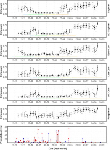
Previously to classification tests assessment, individual SAR features (${\mathrm{\sigma }}_{\text{VV}}^0,$ ${\mathrm{\sigma }}_{\text{VH}}^0$ and ${\mathrm{\gamma }}_{\mathrm{VV}}$) time series were analysed for each class. In each time series of each class, the average and standard deviation of pixel values corresponding to the total polygons (whole dataset) are depicted. Figure 3 shows the backscatter coefficient behaviour at both VV and VH polarization. Moreover, time series of coherence at VV polarization are observed in Figure 4.

Figure 3. The five upper plots correspond to the time series of backscatter coefficient of the classes at VV (magenta) and VH (green) polarization. Points represent the average values, while vertical lines represent standard deviation for all polygons of each class. For crop classes, horizontal line represents the seasonal crop calendar with the seeding period (light blue), vegetative stage (green), reproductive stage (yellow) and harvest period (brown). The lower plot corresponds to the daily precipitation data registered by the Pergamino (red) and Arrecifes (blue) stations.

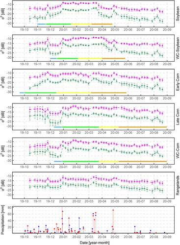
Figure 4. The five upper plots correspond to the time series of coherence of the classes at VV polarization. Points represent the average values, while vertical lines represent standard deviation for all polygons of each class. For crop classes, horizontal line represents the seasonal crop calendar with the seeding period (light blue), vegetative stage (green), reproductive stage (yellow) and harvest period (brown). The lower plot corresponds to the daily precipitation data registered by the Pergamino (red) and Arrecifes (blue) stations.

In Figure 3, similar behaviour was observed for ${\mathrm{\sigma }}_{\text{VV}}^0$ and ${\mathrm{\sigma }}_{\text{VH}}^0$ throughout the time series for all evaluated classes. These features have been broadly studied for corn and soybean monitoring (Jiao et al. 2011; Veloso et al. 2017; Vreugdenhil et al. 2018; Khabbazan et al. 2019; Kumari et al. 2019; Nasirzadehdizaji et al. 2021). However, some differences in backscatter between and in the crops along their life cycles are important to be highlighted.

Firstly, seeding period showed the lowest values for both crops. It is likely to be due to the signal interaction with bare soil (smooth roughness surface). In vegetative stage, a sharp backscatter increase was observed for both crops, mainly during the first half of this stage. This would be related to the crop growing and the consequent leaves development at this period. Under this condition, the higher the biomass, the stronger the backscattered signal due to the volume backscattering mechanism increase (Khabbazan et al. 2019; Xie et al. 2021). It should be noted that time-lapse of mentioned up-ward trend was shorter for late sown than for early sown crops (both soybean and corn). During the late period of vegetative stage and during the reproductive stage, some important differences between soybean and corn were observed, regardless of the sowing period. For soybean, this period is usually characterized by leaves development until mid-late of reproductive stage, while the very end of this reproductive stage is described by a high rate of crop senescence and leaves loss. These crop variations would be linked to the high and unchanged backscatter values until the end of the crop cycle. After that, a marked decrease of backscatter was noticed (mainly for ${\mathrm{\sigma }}_{\text{VH}}^0$). It could be related to the decrease of signal interaction with vegetation, due to both the low biomass close to soybean maturity time (thin dry stem standing) and the crop harvesting. This pattern can be seen during March for Soybean and April for WC-Soybean. On the other hand, backscatter for maize crop showed constant values from late vegetative stage to early reproductive stage and, from this point on, a slight downward trend until harvest period was observed. This behaviour could be related to corn plant architecture for mentioned periods and the plant moisture loss due to the plant drying out. Unlike soybeans, maize leaf senescence rate increases from early reproductive stage (Borrás et al. 2003), and dry leaves remain downwards (only some of the dry leaves fall off the plant). Under this condition, backscattering response could be linked to a decrease of volume backscattering component, and a lower backscattered energy due to the lower moisture presence in the plant. For maize crop, although a backscatter decrease was noticed from the end of the crop cycle, such decrease was not as significant as for soybeans. In the study region, maize fields are generally not harvested from a couple of weeks up to several months after reaching physiological maturity for grain drying out (depending on climatic conditions and crop seeding time). During this period, the whole plant senescence is usually reached, and the backscattering response would be dominated by the contribution of the soil and the corn stalks (Ulaby et al. 1984).

Likewise, some relevant points of backscatter time series should be highlighted:

1. For most of the vegetative and reproductive stages, both ${\mathrm{\sigma }}_{\text{VV}}^0$ and ${\mathrm{\sigma }}_{\text{VH}}^0$ values for soybean were higher than for corn (regardless of seeding periods).

2. In both crops, early and late sown periods can be distinguished due to the time lag of their life cycles. In this sense, backscatter information in specific periods, such as the month of December, could be relevant to discern early and late sown crops. During this month, backscatter values for early sown crops (vegetative stage) are higher than for late sown crops (seeding period).

3. Until December, backscatter values differences between crop sequences (WC-Soybean and WC-Corn) and Late Corn can be observed. Although they both have a similar seeding period, the different field cover prior to crop summer sowing, as well as the presence of residue of harvested winter crop for crop sequences would produces unlike backscatter values. For this period, such differences were even higher between early sown crops (Soybean and Early Corn) and late sown crops (Soybean, Late Corn and WC-Corn).

For Rangelands class, relatively constant values from October to January (summer beginning) were observed. Then, a backscatter increase was noticed, and after that, constant values remained (minor changes) until May. This backscatter behaviour could be linked to the higher vegetation presence in early January. From May to September, a backscatter downward trend was observed. During this period (dry season), moisture loss in vegetation cover would reduce the backscattered energy. It is important to point out that throughout the time series, backscatter values were never higher than those corresponding to the vegetative and reproductive stages of the crops.

Above-mentioned relationships between crop growth and backscatter behaviours are linked to the coherence time series shown in Figure 4. High coherence values were observed during the seeding period of the crops compared to crops growing season. For this period, vegetation cover absence on field would produce similar signal-ground interaction for the interferometric pairs’ images (depending on soil moisture changes and the structure of winter crop residue for crop sequences). As the crops grow, a coherence downward behaviour is evident until reaching the lowest values for each crop. This pattern is clearly noticeable during the first half of vegetative stages. During this period, geometric changes in the fields due to crop growth are likely to occur with a consequent temporal decorrelation increase. From this point on, low coherence values until the end of the crops cycle were observed. For this period, geometric and dielectric changes in canopy like leaves movement caused by the wind and the crop drying out would produce a strong temporal decorrelation. From the end of crop cycle and during the harvest period, a coherence increase was observed in both crops. The latter could be linked to the field harvesting. Harvested fields would produce more stable ground conditions compared to vegetation cover for interferometric pairs’ images (Kavats et al. 2019; Shang et al. 2020; Amherdt et al. 2021).

It should be noted that during December, coherence values for late sown crops (seeding period) were higher than for early sown crops (vegetative/reproductive stage). This could contribute to early and late sowing crops differentiation.

Coherence time series for Rangelands class showed: i) relatively high (compared to values corresponding to crops vegetative/reproductive stages) constant values for the October-December time range; ii) a slight increase in the month of December; iii) higher (compared to December) constant values in the January-May time interval and iv) an upward behaviour from May to June and values with minor changes from June.

Some peaks can be clearly identified in both backscatter (high values) and coherence (low values) time series. These could be linked to rainfall events. For backscatter values, the higher the moisture content, the higher the backscattered energy. Furthermore, variations in soil and canopy moisture due to precipitation have previously been reported as a significant decorrelation source (Ahmed et al. 2011; Simard et al. 2012). Such behaviours are clearly evidenced in both backscatter and coherence time series for Rangelands class (also observed for crop classes) at the end of December, at mid-March, and at the end of April. This patterns was observed in late November as well. In that case, although rainfall events were reported prior to the images acquisition, those precipitation values were not as intense as for the rest of the above mentioned cases.

3.2. Crop classification

According to the defined classifier training strategy, the class with the lowest number of samples corresponded to WC-Corn (point 1 of Section 2.3.3). The summary of the obtained sampling according to the point 2 of Section 2.3.3 is shown in Table 3.

Table 3. Randomly selected polygons from the whole dataset according to the classifier training strategy (points 1 and 2 of Section 2.3.3).

Class	Number of polygons	Area (Ha)
Soybean	32	775.0
WC-Soybean	28	805.4
Early Corn	32	737.4
Late Corn	37	741.4
WC-Corn	32	772.6
Rangelands	28	791.8

Regarding the performed classification sets to evaluate the SAR information for different crops growth stages, the used time ranges for each set are described below:

1. Range 1: complete dataset of SAR images. It corresponds to almost a whole year (October 2019–September 2020). This period contains information from the drying period of winter crops to corn and soybean crops (early and late sown) post-harvest period.

2. Range 2: from 14 October 2019 to 12 January 2020. This period contains information from the drying period of winter crops up to: i) early/mid reproductive stage of early sown corn (full plant development is reached); ii) the end of vegetative stage of early sown soybean (maximum values of both height and fresh biomass are not probably reached) and iii) the beginning of vegetative stage of late sown crops (period characterized by low/medium leaf development). In this set, the contribution of SAR data up to early/middle growth stages of study crops to the proposed classification, as well as the in-season classifications (defined as ‘early-season’ classifications) accuracies were evaluated.

3. Range 3: from 14 October 2019 to 24 March 2020. This period contains information from the drying period of winter crops up to: i) harvest period of early sown crops (whole plant senescence is reached); ii) the end of reproductive stage for WC-Soybean and iii) the beginning of reproductive stage of late sown corns (maximum values of both height and fresh biomass are probably reached). In this set, the contribution of SAR data up to middle/late growth stages of study crops to the proposed classification, and the in-season classification (defined as ‘mid-season’ classifications) accuracies were evaluated.

4. Range 4: from 14 October 2019 to 10 June 2020. This period contains information from the drying period of winter crops to harvest period (whole plant senescence is reached for unharvested fields) of late sown corns, and post-harvest period of the rest of study crops.

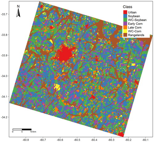
General and individual metrics derived from error matrices (Table S1) for classifications assessment (Section 2.3.4) were depicted in 2 tables. Moreover, classification obtained through backscatter at VV polarization was taken as reference for the scores’ comparison in each classification set (analysed time ranges). This polarization was chosen as reference because the co-polarization is the conventional one for singular polarization SAR systems. In the next subsection, obtained results are described. In Figure 5 an example of the proposed crop classification for the study area is shown.

Figure 5. Example of the proposed crop-type map. It corresponds to the obtained using the ${\mathrm{\sigma }}_{\text{VV}}^0$ + ${\mathrm{\sigma }}_{\text{VH}}^0$ + ${\mathrm{\gamma }}_{\mathrm{VV}}$ SAR features for Range 4 to train the classifier. Urban areas were masked out with the Global Man-made Impervious Surface (GMIS) Dataset from LANDSAT (Brown de Colstoun et al. 2017).

3.2.1. Classification tests

In Table 4 similar relationships between the classification tests can be observed for all the classification sets. Firstly, classification tests obtained using the coherence were the less accurate. For the latter, the decrease (compared to the ${\mathrm{\sigma }}_{\text{VV}}^0$ classification) in overall accuracy and the kappa index, respectively, in each classification set was: 7% and 9 points for Range 1; 8% and 9 points for Range 2; 14% and 17 points for Range 3; and 8% and 10 points for Range 4. Secondly, the rest of classification tests highlighted slightly higher general accuracies (compared to the ${\mathrm{\sigma }}_{\text{VV}}^0$ classification). In this sense, highest differences were seen using backscatter coefficient at both VV and VH polarization and all the analysed features. For these, the increase in the overall accuracy and the kappa index, respectively, in each classification set was, 2% and 3 points for Range 1; 5–6% and 6–7 points for Range 2; 3% and 3–4 points for Range 3; and 2% and 3–4 points for Range 4.

Table 4. Overall accuracy and kappa index scores corresponding to each classification test for the analysed time ranges.

Classifier training input	Range 1		Range 2		Range 3		Range 4
	Overall accuracy (%)	Kappa index	Overall accuracy (%)	Kappa index	Overall accuracy (%)	Kappa index	Overall accuracy (%)	Kappa index
${\mathrm{\sigma }}_{\text{VV}}^0$	95.41	0.94	84.55	0.81	91.68	0.90	95.14	0.94
${\mathrm{\sigma }}_{\text{VH}}^0$	96.48	0.96	87.35	0.85	93.50	0.92	96.14	0.95
${\mathrm{\gamma }}_{\mathrm{VV}}$	88.17	0.85	76.89	0.72	77.68	0.73	86.77	0.84
${\mathrm{\sigma }}_{\text{VV}}^0$ + ${\mathrm{\gamma }}_{\mathrm{VV}}$	97.06	0.96	88.10	0.85	93.89	0.92	96.70	0.96
${\mathrm{\sigma }}_{\text{VH}}^0$ + ${\mathrm{\gamma }}_{\mathrm{VV}}$	96.95	0.96	89.34	0.87	94.28	0.93	96.82	0.96
${\mathrm{\sigma }}_{\text{VV}}^0$ + ${\mathrm{\sigma }}_{\text{VH}}^0$	97.15	0.96	89.49	0.87	94.45	0.93	96.97	0.96
${\mathrm{\sigma }}_{\text{VV}}^0$ + ${\mathrm{\sigma }}_{\text{VH}}^0$ + ${\mathrm{\gamma }}_{\mathrm{VV}}$	97.48	0.97	90.16	0.88	94.76	0.94	97.29	0.97

Regarding the individual scores (Table 5), similar patterns for all the classification sets were evidenced as well. A decrease in most of the classes was observed for the coherence classifications (compared to the ${\mathrm{\sigma }}_{\text{VV}}^0$ classifications). In this context, the highest decrease was observed for WC-Soybean, Late Corn, WC-Corn (except for Range 2) and Rangelands classes. For these classes, the decrease in UA and PA, respectively, in each classification set was, 9% and 12% (WC-Soybean), 15% and 10% (Late Corn), and 20% and 3% (WC-Corn) for the Range 1; 11% and 13% (WC-Soybean), 16% and 8% (Late Corn), and 8% and 12% (Rangelands) for Range 2; 13% and 34% (WC-Soybean), 26% and 8% (Late Corn), and 31% and 16% (WC-Corn) for Range 3; and 7% and 18% (WC-Soybean), 20% and 6% (Late Corn) and 28% and 8% (WC-Corn) for Range 4. In sets corresponding to Range 1, 3 and 4, a significant PA decrease for the class Rangelands was observed (9%, 11% and 9% for each set, respectively). On the other hand, the rest of classification tests showed similar performances (slightly higher) for most of the classes (compared to the ${\mathrm{\sigma }}_{\text{VV}}^0$ classifications). Only classes corresponding to late sown corns (Late Corn and WC-Corn) showed a significant increase. Such pattern was more noticeable for the classification set corresponding to Range 2.

Table 5. User’s and producer’s accuracy for all classification test corresponding to each evaluated classification set.

Classifier training input	User’s accuracy (%)						Producer’s accuracy (%)
	S	WC-S	EC	LC	WC-C	R	S	WC-S	EC	LC	WC-C	R
	Range 1
${\mathrm{\sigma }}_{\text{VV}}^0$	96.8	98.5	96.8	96.2	59.1	97.1	98.3	96.0	97.2	86.7	88.7	97.7
${\mathrm{\sigma }}_{\text{VH}}^0$	98.5	98.3	98.8	95.2	64.8	98.0	97.2	98.0	98.2	87.6	90.8	99.7
${\gamma }_{\mathrm{VV}}$	96.6	89.7	92.3	80.5	38.7	97.1	94.7	83.9	95.9	76.6	85.3	89.2
${\mathrm{\sigma }}_{\text{VV}}^0 + {\gamma }_{\mathrm{VV}}$	97.9	99.0	98.3	97.0	66.6	99.4	98.8	97.5	99.3	91.6	90.7	97.7
${\mathrm{\sigma }}_{\text{VH}}^0 + {\gamma }_{\mathrm{VV}}$	98.6	98.7	99.0	95.6	67.6	98.4	97.7	97.9	99.0	89.8	91.7	99.3
${\mathrm{\sigma }}_{\text{VV}}^0 + {\mathrm{\sigma }}_{\text{VH}}^0$	98.9	98.6	98.7	95.8	69.8	99.1	98.1	98.2	98.6	90.1	91.0	99.7
${\mathrm{\sigma }}_{\text{VV}}^0 + {\mathrm{\sigma }}_{\text{VH}}^0 + {\gamma }_{\mathrm{VV}}$	98.9	98.6	99.0	96.7	69.6	99.6	98.2	98.4	99.4	91.0	91.4	99.5
	Range 2
${\mathrm{\sigma }}_{\text{VV}}^0$	92.9	92.2	91.3	79.8	29.1	87.7	93.9	74.9	93.4	69.2	75.9	92.9
${\mathrm{\sigma }}_{\text{VH}}^0$	96.6	93.0	95.0	81.1	30.4	96.6	93.1	71.1	97.8	83.6	85.6	96.6
${\mathrm{\gamma }}_{\mathrm{VV}}$	93.3	81.2	89.4	63.9	26.1	79.3	90.8	61.7	92.4	61.5	75.6	93.3
${\mathrm{\sigma }}_{\text{VV}}^0 + {\mathrm{\gamma }}_{\mathrm{VV}}$	94.7	93.4	95.3	86.8	34.3	89.8	95.8	77.3	97.8	76.7	77.7	94.7
${\mathrm{\sigma }}_{\text{VH}}^0 + {\mathrm{\gamma }}_{\mathrm{VV}}$	97.0	94.2	95.4	84.8	34.9	96.6	93.7	76.4	98.3	85.4	85.8	97.0
${\mathrm{\sigma }}_{\text{VV}}^0 + {\mathrm{\sigma }}_{\text{VH}}^0$	96.3	94.9	95.3	85.5	33.1	97.8	94.5	76.8	98.6	84.0	85.1	96.3
${\mathrm{\sigma }}_{\text{VV}}^0 + {\mathrm{\sigma }}_{\text{VH}}^0 + {\gamma }_{\mathrm{VV}}$	96.6	95.0	95.5	85.3	36.4	97.8	94.8	78.7	99.0	84.4	84.1	96.6
	Range 3
${\mathrm{\sigma }}_{\text{VV}}^0$	93.7	97.0	94.5	87.1	46.7	95.9	97.8	89.5	96.6	76.4	78.5	97.6
${\mathrm{\sigma }}_{\text{VH}}^0$	97.7	97.4	97.7	85.4	52.6	97.5	96.9	90.3	97.5	83.3	87.1	99.4
${\gamma }_{\mathrm{VV}}$	93.9	84.5	91.2	62.1	15.6	95.8	90.7	55.7	95.4	68.4	62.1	86.9
${\mathrm{\sigma }}_{\text{VV}}^0 + {\gamma }_{\mathrm{VV}}$	96.5	97.6	96.2	88.4	56.8	97.9	97.3	91.6	98.2	84.9	86.0	97.5
${\mathrm{\sigma }}_{\text{VH}}^0 + {\gamma }_{\mathrm{VV}}$	97.7	97.1	97.9	87.3	55.8	98.8	96.8	91.1	99.0	85.2	88.4	99.3
${\mathrm{\sigma }}_{\text{VV}}^0 + {\mathrm{\sigma }}_{\text{VH}}^0$	97.5	97.7	97.2	87.7	56.7	99.2	97.3	92.4	99.0	83.1	89.2	99.5
${\mathrm{\sigma }}_{\text{VV}}^0 + {\mathrm{\sigma }}_{\text{VH}}^0 + {\gamma }_{\mathrm{VV}}$	97.4	97.5	97.4	88.3	59.0	99.6	97.3	92.7	99.4	84.4	89.2	99.4
	Range 4
${\mathrm{\sigma }}_{\text{VV}}^0$	96.4	98.7	95.2	95.9	60.5	97.0	98.4	95.7	97.2	85.7	88.8	97.4
${\mathrm{\sigma }}_{\text{VH}}^0$	98.5	98.4	98.2	94.0	63.5	97.9	97.2	97.3	97.9	87.1	91.1	99.6
${\gamma }_{\mathrm{VV}}$	96.5	91.4	92.8	75.3	32.1	97.4	94.7	77.6	96.1	79.4	80.7	88.9
${\mathrm{\sigma }}_{\text{VV}}^0 + {\gamma }_{\mathrm{VV}}$	97.8	98.9	97.6	96.3	66.7	99.0	98.7	96.7	98.8	91.3	90.7	97.7
${\mathrm{\sigma }}_{\text{VH}}^0 + {\gamma }_{\mathrm{VV}}$	98.6	98.5	98.4	94.2	70.4	98.9	97.3	97.2	98.8	90.8	92.5	99.2
${\mathrm{\sigma }}_{\text{VV}}^0 + {\mathrm{\sigma }}_{\text{VH}}^0$	98.8	98.5	97.9	96.0	68.2	99.3	97.9	98.1	98.9	88.9	91.7	99.6
${\mathrm{\sigma }}_{\text{VV}}^0 + {\mathrm{\sigma }}_{\text{VH}}^0 + {\gamma }_{\mathrm{VV}}$	98.9	98.7	98.0	95.4	73.3	99.5	97.7	97.9	99.3	91.2	92.2	99.5

S: Soybean; WC-S: WC-Soybean; EC: Early Corn; LC: Late Corn; WC-C: WC-Corn; R: Rangelands.

In addition, some relevant points from Tables 4 and 5 should be mentioned:

• Contribution of coherence to backscatter at VV or VH polarization for the proposed classification (for all classification sets). Increases in individual scores for all classes were achieved by adding coherence to backscatter information. These increases were more noticeable for Range 2. The highest differences were observed for late sown corn (both Late Corn and WC-Corn).

• VH polarization yielded better results than VV polarization using backscatter at single polarization (for all classification sets).

• Classification tests using VV and VH polarization backscatter, as well as all the analysed SAR variables produced the best scores (general and individual) in all classification sets. Further, minor differences between them were observed (except for Range 4, in which an increase of 5% in UA for WC-Corn was noticed when adding coherence to backscatter information).

• Highest individual scores corresponded to classes of early sown crops (soybean and corn) for all classifications sets.

• Lowest individual scores corresponded to classes of late sown crops (soybean and corn). Particularly, WC-Corn showed the lowest scores (mainly in UA values) for all the obtained classifications.

• All classification tests showed a significant improvement compared to the classification obtained using only backscatter at VV polarization (excluding the obtained one using coherence information) in classification set corresponding to Range 2. The major increases were for corn classes (particularly late sown corns).

4. Discussion

This study confirmed the added value of coherence to backscatter information for crop classification purposes (Busquier et al. 2020; Mestre-Quereda et al. 2020). Particularly, the contribution of coherence to backscatter information for corn and soybean mapping considering different sowing times, and single or double crop systems was demonstrated for the first time. The accuracies improvement by adding coherence to backscatter information was higher when using single polarization backscatter (VV or VH) for all the classification sets. Such enhancement was more significant for early-season map (Range 2). On the other hand, coherence addition to backscatter information at both VV and VH polarization produced some improvements in accuracy scores (mainly individual scores), but these were not significant enough. In this case, the use of coherence would not be convenient for the proposed classification due to the high computational cost implied in the coherence estimation and the classification process.

This study also evaluated the most suitable variables among the analysed SAR features, as well as the contribution of SAR information corresponding to different crops growth stages for the proposed classification. In this context, the using of backscatter information at both VV and VH polarization would be the most adequate for the proposed classification. As mentioned before, the addition of coherence to backscatter variables is not worthy considering the low accuracy improvement and the high computational burden. In this sense, the integration of both VV and VH polarization has been reported as the most suitable combination for crop classification purposes among the backscatter information (McNairn and Shang 2016). For the latter classification tests (${\mathrm{\sigma }}_{\text{VV}}^0$ + ${\mathrm{\sigma }}_{\text{VH}}^0$ and ${\mathrm{\sigma }}_{\text{VV}}^0+{\mathrm{\sigma }}_{\text{VH}}^0+{\mathrm{\gamma }}_{\mathrm{VV}}$), a significant improvement in accuracies for crop sequences (corn and soybean) classes was observed from classification set corresponding to Range 2 compared to classification set corresponding to Range 3. This suggests that the period between both classification sets would contain valuable information for soybean and maize discerning (double crop systems) but not for late sown corns (Late Corn and WC-Corn) differentiation. Regarding the preferable polarization, VH polarization would be more suitable than VV polarization, mainly for in-season classification (Range 2 and 3). This is consistent with McNairn and Shang (2016) findings, who reported the linear cross-polarization as the best single polarization for crop classification purposes. For all classification sets, classification performances using only coherence for classifier training were the lower. In this context, coherence classifications corresponding to Range 2 and 3 sets reached very similar scores. Indeed, classification corresponding to Range 2 resulted more adequate than the Range 3 one for late sown crops discrimination. Only for the Rangelands class, classification test obtained in the classification set corresponding to the Range 3 highlighted a significant improvement compared to that obtained for Range 2. All scores showed an improvement for the classification sets that contained information on the complete crops growing season (Range 1 and 4). This suggests that most valuable coherence information would be found for the winter crop harvesting period, seeding and emergence of summer crops periods, and from the beginning of summer crops drying out. Coherence information would be not relevant during most of vegetative and reproductive periods of the crops for the proposed classification. This could be linked to the strong temporal decorrelation component during the latter mentioned growth stages for both crops according to the observed in Section 3.1. Such coherence behaviour during the growth period for other crops has been previously reported (Villarroya-Carpio et al. 2022). Moreover, all late sown crops showed an enhancement of accuracies in classification sets corresponding to Range 1 and 4 compared to classification set corresponding to Range 3 (for all classification tests). This evidences the contribution of SAR information (mainly backscatter information) during the mid/late reproductive periods of the crops. Furthermore, general and individual accuracies for classification sets corresponding to Range 1 and 4 were almost the same (for all classification tests). This suggests that there is no valuable SAR information during harvest and post-harvest periods, particularly for maize crop. These periods were evaluated due to the relationship of the SAR response with different crop residues according to previous studies (McNairn et al. 2001, 2002), which could contribute to crop classification.

As mentioned in Section 3.2.1, WC-Corn class achieved the lowest accuracy scores in all classification tests for all classification sets. This could be related to the similar time series (mainly for backscatter information) between this class and the rest of the classes corresponding to late sown crops. As described in Section 3.1, the WC-Corn backscatter and coherence time series exhibited similar behaviour to that of WC-Soybean from October to December, and from December onward time series were analogous to those of Late Corn. This could produce misclassification between these classes (mainly between Late Corn and WC-Corn).

Obtained results can be compared with previous works on soybean and corn mapping. However, it must be considered that each study about crop-type mapping with SAR data has specific characteristics related to the study site (evaluated crop, climatic conditions, among others) and the employed data (SAR variables, signal frequency, acquisitions number, among others). In this context, achieved results are in accordance with those obtained by Amherdt et al. (2021), but some relevant differences must be pointed out: first, the capability of distinguishing Late Corn and WC-Corn, being the major challenge due to their very similar calendars; second, the SAR information contribution for different growth stages of the crops, evidenced by the performed classification sets; and third, the coherence contribution to crop mapping. Further, obtained mid-season map (Range 3) was quite similar to that obtained by Dingle Robertson et al. (2020) by combining backscatter at VV and VH polarization for corn and soybean mapping in the region; while, achieved general accuracy using VH polarization backscatter information for the whole crops growing season (Range 1 or 4) was similar to that reported by Whelen and Siqueira (2018) for corn and soybean classification in North Dakota, United States. It is worth noting that in these works only crop type was distinguished using C-band SAR data, without considering different sowing dates and crop systems as in the present study. On the other hand, a dense dataset of SAR imagery would be suited for the ‘early-season’ crops mapping (mainly for soybean crop) comparing the obtained results with those reported by McNairn et al. (2014). It is important to highlight that classification corresponding to the aforementioned work was attained using the combination of C-band and X-band SAR images (small dataset of images) and a Decision Tree classifier. In the present study, not only crop-type mapping but also crop discerning according to seeding time and crop system (single crop or crop sequence) was feasible with a high accuracy. In this sense, accuracy scores for maize crop classes were similar for early and late planted corn, but significantly worse for the double crop system (employing backscatter information of the whole crop season) compared to those obtained by L. Li et al. (2019). In addition, obtained results in the present study were similar and even more accurate (mainly using backscatter at both VV and VH polarization) compared to those obtained by de Abelleyra et al. (2020), who employed optical images time series for corn and soybean mapping over the same region. In this context, Dingle Robertson et al. (2020) also reported better performance when using SAR image time series compared to optical image time series for soybean and maize mapping. As already mentioned, optical images have been extensively studied for cropland mapping. However, SAR sensor characteristics would allow to separate one crop type from another due to the recognition of changes in and between the structure of the crops throughout their growth stages (McNairn et al. 2014). Therefore, although not a substitute for optical data, SAR data proved to be a suitable source for crop classification, particularly for mapping corn and soybeans.

Potential limitations from this work are mainly related to:

• The SAR images time span. In this context, the evaluation for more than one summer crops season would allow more robust conclusions to be drawn. Also, a larger number of images for the winter crop growing season could provide critical information to discriminate the WC-Corn and Late Corn.

• The unavailability of a larger reference dataset obtained in-situ. In this sense, the possible erroneous definition of classes for some samples due to misinterpretation of the optical images would decrease the accuracy of the classifications.

5. Conclusions

In this work the coherence contribution to backscatter information for soybean and corn mapping was demonstrated. In addition, the contribution of crops growth stages to proposed classification and in-season maps accuracies were assessed. In this context, the main challenges were both the crop-type discerning, as well as its discrimination according to crop systems (single crop of crop sequence) and sowing time.

Results evidenced the coherence added value to single backscatter coefficient (VV or VH), mainly for late sown corns (Late Corn and WC-Corn) discerning. In this sense, coherence addition to backscatter information could be a suitable tool for soybean and corn mapping using C-band singular VV polarization SAR images. However, the combination of backscatter at VV and VH polarization would be the preferable variables for the proposed classification. In this case, the addition of coherence would not be convenient due to the minor accuracies improvement and the high computational burden involved in coherence estimation and classifier training. Among the backscatter variables, VH polarization resulted more adequate than VV polarization. Also, results showed that there is useful SAR information up to the end of the crops growing season for proposed classification. Despite that, there is valuable SAR information until early and middle stages of crops growth. In this context, time series of C-band SAR images would be an adequate source for early season classification of corn and soybean. Both early season and middle season classifications achieved a high accuracy, mainly using backscatter information at VV and VH polarization or all the analysed SAR features. The availability of early season maps allows to better plan various input supply tasks, and/or organize logistics and transportation to consumer markets.

Moreover, further studies evaluating different crop types should be carried out to confirm the added value of coherence to crop mapping purposes, as well as the suitability of SAR data to obtain accurate in-season maps.

Disclosure statement

No potential conflict of interest was reported by the author(s).

References

- Ahmed R, Siqueira P, Hensley S, Chapman B, Bergen K. 2011. A survey of temporal decorrelation from spaceborne L-Band Repeat-Pass InSAR. Remote Sen Envi. 115(11):2887–2896. doi:10.1016/j.rse.2010.03.017.
- Amherdt S, Di Leo NC, Balbarani S, Pereira A, Cornero C, Pacino MC. 2021. Exploiting Sentinel-1 data time-series for crop classification and harvest date detection. Int J Remote Sens. 42(19):7313–7331.
- Aoki AM, Robledo JI, Izaurralde RC, Balzarini MG. 2021. Temporal integration of remote‐sensing land cover maps to identify crop rotation patterns in a semiarid region of Argentina. Agron J. 113(4):3232–3243.
- Attema E, Cafforio C, Gottwald M, Guccione P, Monti Guarnieri A, Rocca F, Snoeij P. 2010. Flexible dynamic block adaptive quantization for Sentinel-1 SAR missions. IEEE Geosci Remote Sens Lett. 7(4):766–770.
- Bitar MV, Cabrini SM, Orlando L, Lingua M, Paolilli C, Fillat F, Elustondo L, Bevaqua F, Senigagliesi C. 2020. Los sistemas productivos del partido de Pergamino: resultados de una encuesta a productores. Indicadores económicos e informes técnicos INTA EEA Pergamino, N° 2, enero 2020. https://inta.gob.ar/sites/default/files/inta_pergamino_los_sistemas_productivos_del_partido_de_pergamino_resultados_de_una_encuesta_a_productores_2.pdf.
- Blaes X, Vanhalle L, Defourny P. 2005. Efficiency of crop identification based on optical and SAR image time series. Remote Sens Environ. 96(3-4):352–365.
- Borrás L, Maddonni GA, Otegui ME. 2003. Leaf senescence in maize hybrids: plant population, row spacing and kernel set effects. Field Crops Res. 82(1):13–26.
- Bowles TM, Mooshammer M, Socolar Y, Calderón F, Cavigelli MA, Culman SW, Deen W, Drury CF, Garcia AG, Gaudin AC, et al. 2020. Long-term evidence shows that crop-rotation diversification increases agricultural resilience to adverse growing conditions in North America. One Earth. 2(3):284–293.
- Breiman L. 2001. Random forests. Mach Learn. 45(1):5–32.
- Brown de Colstoun EC, Huang C, Wang P, Tilton JC, Tan B, Phillips J, Niemczura S, Ling P-Y, Wolfe RE. 2017. Global man-made impervious surface (GMIS) dataset from Landsat. Palisades, NY: NASA Socioeconomic Data and Applications Center (SEDAC); [accessed 2021 Oct 19].
- Busquier M, Lopez-Sanchez JM, Mestre-Quereda A, Navarro E, González-Dugo MP, Mateos L. 2020. Exploring TanDEM-X interferometric products for crop-type mapping. Remote Sens. 12(11):1774.
- Cai Y, Guan K, Peng J, Wang S, Seifert C, Wardlow B, Li Z. 2018. A high-performance and in-season classification system of field-level crop types using time-series Landsat data and a machine learning approach. Remote Sens Environ. 210:35–47.
- Chang J, Hansen MC, Pittman K, Carroll M, DiMiceli C. 2007. Corn and soybean mapping in the United States using MODIS time‐series data sets. Agron J. 99(6):1654–1664.
- Congalton RG, Green K. 2020. Assessing the accuracy of remotely sensed data: principles and practices. 3rd ed. London, UK: CRC Press.
- de Abelleyra D, Veron S, Banchero S, Mosciaro MJ, Propato T, Ferraina A, Taffarel MCG, Dacunto L, Franzoni A, Volante J. 2020. First large extent and high resolution cropland and crop type map of Argentina. 2020 IEEE Latin American GRSS & ISPRS Remote Sensing Conference (LAGIRS). 22–26 March 2020, Santiago, Chile: IEEE.
- Di Yenno F, Terré E. 2021. Argentina se encamina a un récord de siembras en la 2021/22. Informativo semanal: Mercados; [accessed 2021 July 23]. https://www.bcr.com.ar/es/print/pdf/node/87073.
- Dingle Robertson L, M. Davidson A, McNairn H, Hosseini M, Mitchell S, de Abelleyra D, Verón S, Le Maire G, Plannells M, Valero S, et al. 2020. C-band synthetic aperture radar (SAR) imagery for the classification of diverse cropping systems. Int J Remote Sens. 41(24):9628–9649.
- Engdahl M. 2013. Multitemporal InSAR in land-cover and vegetation mapping [Ph.D. thesis]. Espoo, Finland: Aalto University.
- FAO. 2022. Crops and livestock products; [accessed 2022 May 10]. https://www.fao.org/faostat/en/#data/QCL.
- Frison P-L, Fruneau B, Kmiha S, Soudani K, Dufrêne E, Le Toan T, Koleck T, Villard L, Mougin E, Rudant J-P. 2018. Potential of Sentinel-1 data for monitoring temperate mixed forest phenology. Remote Sens. 10(12):2049.
- Gayo S, López M. 2018. Dinámica de los planteos de maíz en la Argentina: de dónde venimos y hacia dónde vamos. Congreso Maizar 2018; May 22; Buenos Aires, Argentina, http://agrolinux3.agrositio.com/maizar/congresomaizar/2018/presentaciones/competitividad/gayo_lopez.pdf.
- Geudtner D, Torres R. 2012. Sentinel-1 system overview and performance. 2012 IEEE International Geoscience and Remote Sensing Symposium. 22-27 July 2012, Munich, Germany: IEEE.
- Hanssen RF. 2001. Radar interferometry. Data Interpretation and Error Analysis. Remote Sensing Digital Image Processing. Dordrecht, Boston: Springer. doi:10.1007/0-306-47633-9
- Jacob AW, Vicente-Guijalba F, Lopez-Martinez C, Lopez-Sanchez JM, Litzinger M, Kristen H, Mestre-Quereda A, Ziolkowski D, Lavalle M, Notarnicola C, et al. 2020. Sentinel-1 InSAR coherence for land cover mapping: a comparison of multiple feature-based classifiers. IEEE J Sel Top Appl Earth Observ Remote Sens. 13:535–552.
- Jiao X, McNairn H, Shang J, Pattey E, Liu J, Champagne C. 2011. The sensitivity of RADARSAT-2 polarimetric SAR data to corn and soybean leaf area index. Can J Remote Sens. 37(1):69–81.
- Kavats O, Khramov D, Sergieieva K, Vasyliev V. 2019. Monitoring harvesting by time series of Sentinel-1 SAR data. Remote Sens. 11(21):2496.
- Khabbazan S, Vermunt P, Steele-Dunne S, Ratering Arntz L, Marinetti C, van der Valk D, Iannini L, Molijn R, Westerdijk K, van der Sande C. 2019. Crop monitoring using Sentinel-1 data: a case study from The Netherlands. Remote Sens. 11(16):1887.
- Kumari M, Murthy CS, Pandey V, Bairagi GD. 2019. Soybean cropland mapping using multi-temporal Sentinel-1 data. Int Arch Photogramm Remote Sens Spatial Inf Sci. XLII-3/W6:109–114.
- Li J, Huang L, Zhang J, Coulter JA, Li L, Gan Y. 2019. Diversifying crop rotation improves system robustness. Agron Sustain Dev. 39(4). doi:10.1007/s13593-019-0584-0
- Li L, Kong Q, Wang P, Xun L, Wang L, Xu L, Zhao Z. 2019. Precise identification of maize in the North China Plain based on Sentinel-1A SAR time series data. Int J Remote Sens. 40(5-6):1996–2013.
- McNairn H, Champagne C, Shang J, Holmstrom D, Reichert G. 2009. Integration of optical and synthetic aperture radar (SAR) imagery for delivering operational annual crop inventories. ISPRS J Photogramm Remote Sens. 64(5):434–449.
- McNairn H, Duguay C, Boisvert J, Huffman E, Brisco B. 2001. Defining the sensitivity of multi-frequency and multi-polarized radar backscatter to post-harvest crop residue. Can J Remote Sens. 27(3):247–263.
- McNairn H, Duguay C, Brisco B, Pultz TJ. 2002. The effect of soil and crop residue characteristics on polarimetric radar response. Remote Sens Environ. 80(2):308–320.
- McNairn H, Kross A, Lapen D, Caves R, Shang J. 2014. Early season monitoring of corn and soybeans with TerraSAR-X and RADARSAT-2. Int J Appl Earth Obs Geoinf. 28:252–259.
- McNairn H, Shang J. 2016. A review of multitemporal synthetic aperture radar (SAR) for crop monitoring. In Multitemporal remote sensing. Remote Sensing and Digital Image Processing, vol 20. Springer, Cham. p. 317–340. doi: 10.1007/978-3-319-47037-5_15
- Mestre-Quereda A, Lopez-Sanchez JM, Vicente-Guijalba F, Jacob AW, Engdahl ME. 2020. Time-series of sentinel-1 interferometric coherence and backscatter for crop-type mapping. IEEE J Sel Top Appl Earth Observ Remote Sens. 13:4070–4084.
- Morishita Y, Hanssen RF. 2015. Temporal decorrelation in L-, C-, and X-band satellite radar interferometry for pasture on drained peat soils. IEEE Trans Geosci Remote Sens. 53(2):1096–1104.
- Nasirzadehdizaji R, Cakir Z, Balik Sanli F, Abdikan S, Pepe A, Calò F. 2021. Sentinel-1 interferometric coherence and backscattering analysis for crop monitoring. Comput Electron Agric. 185:106118.
- Ok AO, Akar O, Gungor O. 2012. Evaluation of random forest method for agricultural crop classification. Eur J Remote Sens. 45(1):421–432.
- Otegui ME, Riglos M, Mercau JL. 2021. Genetically modified maize hybrids and delayed sowing reduced drought effects across a rainfall gradient in temperate Argentina. J Exp Bot. 72(14):5180–5188.
- Ouaadi N, Jarlan L, Ezzahar J, Zribi M, Khabba S, Bouras E, Bousbih S, Frison P-L. 2020. Monitoring of wheat crops using the backscattering coefficient and the interferometric coherence derived from Sentinel-1 in semi-arid areas. Remote Sens Environ. 251:112050.
- Pott LP, Amado TJC, Schwalbert RA, Corassa GM, Ciampitti IA. 2021. Satellite-based data fusion crop type classification and mapping in Rio Grande do Sul, Brazil. ISPRS J Photogramm Remote Sens. 176:196–210.
- Rosen PA, Hensley S, Joughin IR, Li FK, Madsen SN, Rodriguez E, Goldstein RM. 2000. Synthetic aperture radar interferometry. Proc IEEE. 88(3):333–382.
- Seymour MS, Cumming IG. 2002. Maximum likelihood estimation for SAR interferometry. Proceedings of IGARSS ’94 - 1994 IEEE International Geoscience and Remote Sensing Symposium. 08-12 August 1994, Pasadena, CA, USA: IEEE.
- Shang J, Liu J, Poncos V, Geng X, Qian B, Chen Q, Dong T, Macdonald D, Martin T, Kovacs J, et al. 2020. Detection of crop seeding and harvest through analysis of time-series Sentinel-1 interferometric SAR data. Remote Sens. 12(10):1551.
- She B, Anhui C, Yang Y, Zhao Z, Huang L, Liang D, Zhang D. 2020. Identification and mapping of soybean and maize crops based on Sentinel-2 data. Int J Agric Biol Eng. 13(6):171–182.
- Simard M, Hensley S, Lavalle M, Dubayah R, Pinto N, Hofton M. 2012. An empirical assessment of temporal decorrelation using the uninhabited aerial vehicle synthetic aperture radar over forested landscapes. Remote Sens. 4(4):975–986. doi:10.3390/rs4040975.
- Ulaby FT, Allen CT, Eger G, III, Kanemasu E. 1984. Relating the microwave backscattering coefficient to leaf area index. Remote Sens Environ. 14(1-3):113–133.
- Veloso A, Mermoz S, Bouvet A, Le Toan T, Planells M, Dejoux J, Ceschia E. 2017. Understanding the temporal behaviour of crops using Sentinel-1 and Sentinel-2-like data for agricultural applications. Remote Sens Environ. 199:415–426.
- Villarroya-Carpio A, Lopez-Sanchez JM, Engdahl ME. 2022. Sentinel-1 interferometric coherence as a vegetation index for agriculture. Remote Sens Environ. 280:113208.
- Vreugdenhil M, Wagner W, Bauer-Marschallinger B, Pfeil I, Teubner I, Rüdiger C, Strauss P. 2018. Sensitivity of Sentinel-1 backscatter to vegetation dynamics: an Austrian case study. Remote Sens. 10(9):1396.
- Wang S, Azzari G, Lobell DB. 2019. Crop type mapping without field-level labels: random forest transfer and unsupervised clustering techniques. Remote Sens Environ. 222:303–317.
- Wang S, Di Tommaso S, Deines JM, Lobell DB. 2020. Mapping twenty years of corn and soybean across the US Midwest using the Landsat archive. Sci Data. 7(1):307.
- Weiss M, Jacob F, Duveiller G. 2020. Remote sensing for agricultural applications: a meta-review. Remote Sens Environ. 236:111402.
- Whelen T, Siqueira P. 2018. Time-series classification of Sentinel-1 agricultural data over North Dakota. Remote Sens Lett. 9(5):411–420.
- Xie Q, Lai K, Wang J, Lopez-Sanchez JM, Shang J, Liao C, Zhu J, Fu H, Peng X. 2021. Crop monitoring and classification using polarimetric RADARSAT-2 time-series data across growing season: a case study in Southwestern Ontario, Canada. Remote Sens. 13(7):1394.
- Zebker HA, Villasenor J. 1992. Decorrelation in interferometric radar echoes. IEEE Trans Geosci Remote Sens. 30(5):950–959.
- Zhong L, Hu L, Yu L, Gong P, Biging GS. 2016. Automated mapping of soybean and corn using phenology. ISPRS J Photogramm Remote Sens. 119:151–164.