Challenges for chlorophyll-a remote sensing in a highly variable turbidity estuary, an implementation with sentinel-2

Abstract

Coastal waters have high ecological and economic relevance and are globally threatened by intense human activities leading to eutrophication. The decameter resolution of Sentinel-2 Multispectral Instrument (S2-MSI) provides an advantage to detect spatially heterogeneous phenomena that are limited in extent, such as harmful cyanobacterial blooms (cyanoHABs). Chlorophyll-a is typically used in remote sensing of blooms; however, it remains to be evaluated in several coastal regions of the world. The Río de la Plata estuary (South America) provides a key case study due to its highly variable concentrations of suspended sediments, and the increasing frequency of cyanoHABs. Here, we evaluate the potential and limitations of S2-MSI indices to retrieve chlorophyll-a in these optically complex waters, obtaining regional algorithms and comparing them to previously available ones. We propose an approach to follow the evolution of chlorophyll-a thresholds (10 and 24 μg/L) that can contribute to monitoring programs and early warning strategies of cyanoHABs.

Keywords:

• Water quality
• algal bloom
• cyanobacteria
• Río de la Plata
• turbid waters

1. Introduction

Satellite images can support management and decision making, helping reduce human health risks and direct field resources regarding potentially harmful algal blooms (HABs) (Schaeffer et al. 2015). Within HABs, cyanobacterial blooms (cyanoHABs) are increasing in frequency, magnitude and duration globally in fresh and coastal waters (O’Neil et al. 2012; Huisman et al. 2018).

Algal blooms are commonly quantified through the concentration of chlorophyll-a (chl-a) (Ruddick et al. 2008; Khan et al. 2021), which has the advantage of being one of the most commonly estimated parameters using remote sensing techniques since the 1970s (Gholizadeh et al. 2016). Although chl-a concentrations alone cannot confirm cyanobacteria dominance, remotely sensed chl-a can help detect potential cyanoHABs and their initiation, especially in zones were they are often reported, complementing other monitoring techniques. Moreover, the work of Stumpf et al. (2016) points out that chl-a seems to be more sensitive in detecting changes in biomass in cyanobacterial blooms.

Regarding aquatic color remote sensing of chl-a, estuaries and coastal areas are defined as Case 2 waters (Morel and Prieur 1977), where chl-a does not typically dominate the optical properties of the water, and the presence of inorganic particulate matter plays an important role. For satellite retrieval of chl-a in Case 2 waters, several studies have suggested algorithms that use the red and near infrared (NIR) region of the reflectance spectrum (Gons et al. 2002; Dall’Olmo et al. 2005; Gitelson et al. 2007; Matthews et al. 2012; Mishra and Mishra 2012). However, given the optical complexity within Case 2 waters, and the often empirical nature of the algorithms’ parameterizations, the need for regional tuning should be evaluated in water bodies where they have not been previously applied (Dogliotti et al. 2021).

Despite the described challenges, phytoplankton blooms in estuarine and coastal waters around the globe have been widely studied using ocean colour satellites with spatial resolutions in the order of 10²–10³ m, such as CZCS, SeaWiFS, AVHRR, MERIS, and MODIS (Stumpf and Tyler 1988; Gohin et al. 2003; Gower et al. 2005; Shanmugam 2011; Coronado-Franco et al. 2018), including cyanobacterial blooms (Kahru and Elmgren 2014; Matthews and Odermatt 2015; Cannizzaro et al. 2019). Studies with the decameter-resolution satellite sensors, such as Landsat-8 Operational Land Manager (L8-OLI) and Sentinel-2 Multispectral Instrument (S2-MSI), are currently more scarce (Khan et al. 2021), in part due to their more recent availability (e.g. S2-MSI), and because they are missions primarily designed for terrestrial applications that lack bands at some of the wavelengths commonly used to detect spectral features related to phytoplankton pigments, particularly cyanobacteria (Matthews et al. 2012; Wynne et al. 2008; Lunetta et al. 2015; Urquhart et al. 2017). However, recent works have begun to show their potential for chl-a estimation (Gernez et al. 2017; Pahlevan et al. 2020; Bramich et al. 2021; Pahlevan et al. 2022) and phytoplankton bloom detection (Teta et al. 2017; Borfecchia et al. 2019) in coastal waters.

The Río de la Plata Estuary (Figure 1(a)) has the fifth largest basin of the world (3.1$\times {10}^6$ km²) and drains the second largest flow in South America (Framiñan and Brown 1996). The estuary has great economic and environmental importance, providing numerous services, such as transportation, fisheries, tourism, drinking water supply, and being a relevant habitat for native and migratory species (García-Alonso et al. 2019). It has been exposed to both human and climatic pressures that lead to an increase in nutrient loads and moderate eutrophication (Nagy et al. 2002; García-Alonso et al. 2019). In the last decade, the presence of cyanobacterial blooms had been often reported in its coastal areas (Pirez et al. 2013; Sathicq et al. 2014; Aubriot et al. 2020; Kruk et al. 2021). Moreover, recent research has revealed the ecological diversification of the toxic complex Microcystis aeruginosa along the coast of the Río de la Plata, where they have adapted to different temperature, turbidity and salinity levels (Martínez de la Escalera et al. 2022).

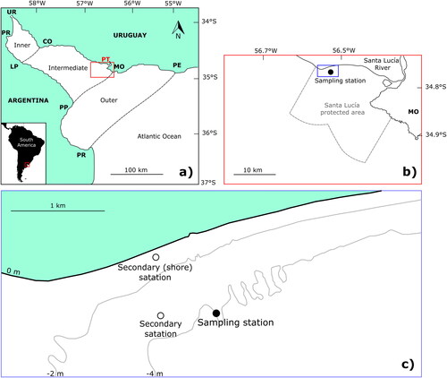
Figure 1. (a) General location of the Río de la Plata and the study region, where the main tributaries UR (Uruguay river) and PR (Paraná river) are indicated, as well as relevant locations along the northern and southern coasts: CO (Colonia) and LP (La Plata) limiting the inner estuary, MO (Montevideo) and PP (Punta Piedras) limiting the intermediate zone, and PE (Punta del Este) and PR (Punta Rasa) indicating the boundary with the Atlantic Ocean. (b) Detail of the study zone of Punta del Tigre (PT), located to the W of MO (Montevideo), the capital city of Uruguay, and within the protected area of the Santa Lucía river. (c) Detail of the coast and bathymetry near the sampling stations.

Regarding remote sensing of chl-a in the Río de la Plata, previous studies have focused on the external region of the estuary and the Southwest Atlantic continental platform (Armstrong et al. 2004; Garcia et al. 2006; Carreto et al. 2008; Garcia and Garcia 2008; Giannini et al. 2013; Machado et al. 2013). Overestimation of satellite chl-a products was highlighted as a problem caused by the turbidity plume of the estuary (Huret et al. 2005; Carreto et al. 2008; Giannini et al. 2013), which receives annually up to 160 million tons of suspended sediments from its main tributaries (Fossati et al. 2014). Regarding remote sensing of algal blooms, Aubriot et al. (2020) described an exceptional cyanoHAB that occurred in 2019 along the northern coast of the estuary by applying the normalized difference chlorophyll index (NDCI) developed by Mishra and Mishra (2012) to S2-MSI images of late January and early February, 2019, but without estimating chl-a concentrations.

To this date, none of these previous studies have evaluated multi-spectral chl-a indices for the Río de la Plata inner and intermediate regions, where high turbidity levels are typically found (Dogliotti et al. 2016). The exception is the recent conference work by Dogliotti et al. (2021) that considered both multi-spectral (matching Sentinel-3 bands) and hyperspectral indices during a cyanobacterial bloom in the southern coast of the estuary. They found better results with hyperspectral algorithms, and concluded that further evaluation and calibration of the algorithms is needed.

Our objectives in this work were: (1) to study the potential of the decameter resolution S2-MSI to retrieve chl-a concentrations from band-combinations of water-leaving reflectance in a coastal region of the Río de la Plata, which has highly variable turbidity levels and has been optically classified as sediment-rich and eutrophic water type (Maciel and Pedocchi 2022); and (2) apply them to detect chl-a levels that are associated to health risks during potential HABs. The consideration of semi-empirical indices based on band-combinations responded to the interest in developing an easy-to-implement monitoring tool that could detect the initial stages of HABs, which in the Río de la Plata are frequently cyanoHABs, and associated chl-a concentrations that are relevant for public health. We relied on a two-year long dataset of in-situ measurements, which covered a wide range of environmental conditions. We also studied the impact of uncorrelated suspended sediments and colour dissolved organic matter (CDOM) variability on chl-a indices which gave critical insight for the Río de la Plata application, and could be useful for other water bodies.

2 Materials and methods

2.1. Field and laboratory data

The study site was the zone of Punta del Tigre (PT), located in the northern coast of the Río de la Plata, closer to the transition between the intermediate and outer zones of the estuary (Figure 1(a)). The sampling site (Latitude 34${}^{°}$45’45.5”S and Longitude 56${}^{°}$32’16.7”W, Figure 1(b)) was located at the W boundary of the Santa Lucía river sound, an area of ecological importance as fish nursery (Jaureguizar et al. 2016). Besides the local influence of the Santa Lucía river, the area is also affected by the general estuarine dynamics, for instance, the turbidity front, typically found near Montevideo (MO), often reaches PT together with saline water intrusions (Maciel et al. 2021). The study period spanned from February 2018 to March 2020, where water samples, continuous records, and radiometric measurements were taken. The depth at the sampling station was around 4 m, and it was located approximately 900 m off from the shore (Figure 1(c)). The coast there consists of a sand beach, but fine cohesive sediments were found to dominate at the sampling station.

Radiometric measurements were obtained at a weekly-to-monthly basis with a set of three RAMSES TriOS hyperspectral radiometers to measure downwelling irradiance, water and sky radiances, following the recommendations in Mobley (1999). These measurements are available in SeaBASS (DOI: 10.5067/SeaBASS/RDLP PT/DATA001). Simultaneously, surface water samples, triplicated at most dates, were collected to measure chl-a. Chl-a was extracted with 90% hot ethanol and measured spectrophotometrically (ISO-10260 1992). Remote sensing reflectance ($R_{\text{rs}}(\lambda )$) was computed from radiometric data, considering the spectral response functions of S2-MSI. For further details of radiometric data processing, refer to Maciel and Pedocchi (2022). A total of 47 resultant $R_{\text{rs}}(\lambda )$ spectra were obtained, corresponding to 45 different field campaigns over the study period, and 43 of them matched chl-a samples.

In order to characterize other colour-related water constituents of the study site, SS and CDOM samples were also simultaneously collected. Total and fixed suspended sediments (TSS and FSS) concentrations were measured gravimetrically (Menéndez 2017), using glass fibre filters with effective particle retention of 1.5 μm. CDOM fluorescence was measured with a table fluorometre (Turner Trilogy, CDOM module excitation: 350/80 nm, emission: 410–450 nm) for samples previously filtered through glass fibre filters with effective particle retention of 0.7 μm. Distilled water was used as blank and subtracted from the sample values. Fluorescence was reported in arbitrary units. Additionally, since September 2019, the CDOM absorption coefficient at 443 nm was measured spectrophotometrically (Mannino et al. 2019), previously filtering the samples through nylon syringe filters with effective pore size of 0.22 μm. The relationship between CDOM arbitrary fluorescence values and absorption coefficient was found to be linear (R²=0.9, n = 20), and it was used to report absorption coefficients in this work.

The sampling point was also a mooring station, where continuous (every half hour) data records were obtained with a SBE 19plus V2 SeaCAT CTD (conductivity, temperature and depth sensor, Sea-Bird Scientific). Salinity (in psu) was also computed from CTD measurements. An ECO Triplet optical sensor with bio-wiper (WETLabs) was integrated (in November 2018) to the CTD to measure turbidity (in NTU) from particles side-scattering at a wavelength of 870 nm. All continuous measurements were obtained approximately at 0.5 m from the bottom. Nevertheless, from CTD profiles measured during field campaigns, the water column was found usually non-stratified.

Chl-a was additionally measured at a secondary station, located approximately 500 m from the main station (Latitude 34${}^{°}$45’46.2”S and Longitude 56${}^{°}$32’37.9”W), as well as at near the shore, at a less frequent basis (monthly to bimonthly) (Figure 1(c)). Values at these two secondary stations were used as a reference for spatial variability. Furthermore, samples for phytoplankton were taken by triplicate at the three stations. Phytoplankton was identified to the lowest taxonomical level possible and counted using an inverted microscope (Olympus CKX41) following standard methods (Sournia 1978). Biovolume was then calculated according to Hillebrand et al. (1999). The relative contribution of cyanobacteria was computed, and it was considered dominant when it was above 50% of the total biovolume.

Given the proximity of the Santa Lucía river mouth to the study site, its discharge was considered as complementary field data. River flow was estimated from a discharge rating curve and daily level data, which was obtained from the Dirección Nacional del Agua (DINAGUA, https://app.mvotma.gub.uy/informacion_hidrica/), Uruguay, at the Santa Lucía city station (50 km upstream of the study site).

2.2. Satellite data

Level 1 C S2 images were downloaded from https://scihub.copernicus.eu/. They were converted to Level 2 (water-leaving reflectances, ${\rho }_{\mathrm{w}}(\lambda )=\pi R_{\text{rs}}(\lambda )$) using the software ACOLITE (https://odnature.naturalsciences.be/remsem/software-and-data/acolite, version 20190326.0), which was developed for inland and coastal waters remote sensing applications (Vanhellemont and Ruddick 2015; Vanhellemont 2019). A sub-scene limited by the following coordinates was used for satellite imagery: latitude between 34.74${}^{°}$ S and 35${}^{°}$ S and longitude from 56.3${}^{°}$ W to 56.8${}^{°}$ W. The DSF algorithm with the additional sun glint (SG) correction (DSF + SG) was applied to the images. This atmospheric correction method was previously validated for the study region in the previous work of Maciel and Pedocchi (2022). After discarding images greatly affected by clouds, a total of sixty S2 images were available for the study area in the period February 2018–April 2020.

2.3. Chl-a indices

Four different chl-a indices based on S2-MSI band-combinations of water-leaving reflectances were considered in this work. The use of band combination indices poses an advantage regarding implementation simplicity in monitoring strategies.

The normalized difference chlorophyll index (NDCI) using the red and red-edge bands was proposed by Mishra and Mishra (2012) for estuarine and coastal turbid productive waters and can be computed as: (1) $$\text{NDCI}=\frac{{\rho }_{\mathrm{w}}(665)-{\rho }_{\mathrm{w}}(705)}{{\rho }_{\mathrm{w}}(665)+{\rho }_{\mathrm{w}}(705)}.$$(1)

A 3-band index (3BI) combining the red, red-edge and a NIR band was first proposed for applications in turbid productive water by Dall’Olmo et al. (2003), being defined as follows: (2) $$3\text{BI}=\left(\frac{1}{{\rho }_{\mathrm{w}}(665)}-\frac{1}{{\rho }_{\mathrm{w}}(705)}\right)\times {\rho }_{\mathrm{w}}(740),$$(2) where ${\rho }_{\mathrm{w}}(\lambda )$ is the water-leaving reflectance for a given band associated to S2-MSI centre wavelength λ.

Another 3-band index has been proposed for a reservoir located upstream of the study region, the Salto Grande dam in the Uruguay river (Drozd et al. 2020). It was considered in this work for being a regionally developed algorithm for a tributary of the Río de la Plata, considering S2-MSI bands. The index proposed by Drozd et al. (2020) (${\mathrm{I}}_{\text{Drozd}}$), as we will call it hereon) takes the form of a normalized difference between the green and red bands, but adding the red edge reflectance in both the numerator and denominator, as follows: (3) $${\mathrm{I}}_{\text{Drozd}}=\frac{{\rho }_{\mathrm{w}}(560)-{\rho }_{\mathrm{w}}(665)+{\rho }_{\mathrm{w}}(705)}{{\rho }_{\mathrm{w}}(560)+{\rho }_{\mathrm{w}}(665)+{\rho }_{\mathrm{w}}(705)}.$$(3)

Finally, a spectral shape (SS) index was considered, also known as reflectance line heights (Matthews 2011). These type of indices measure the reflectance peak at a given band, centred at wavelength λ, relative to a linear baseline between adjacent bands, centred at wavelengths ${\lambda }^{-}$ and ${\lambda }^{+},$ having the following general form (Wynne et al. 2008): (4) $$\text{SS}(\lambda )={\rho }_{\mathrm{w}}(\lambda )-{\rho }_{\mathrm{w}}(\lambda \prime ); {\rho }_{\mathrm{w}}(\lambda \prime )=\left[{\rho }_{\mathrm{w}}({\lambda }^{+})-{\rho }_{\mathrm{w}}({\lambda }^{-})\right]\times \frac{\lambda -{\lambda }^{-}}{{\lambda }^{+}-{\lambda }^{-}}+{\rho }_{\mathrm{w}}({\lambda }^{-}).$$(4)

For S2-MSI, we used $\text{SS}(665),$ with ${\lambda }^{-}=560$ nm, and ${\lambda }^{+}=705$ nm. A comparison with other commonly used $\text{SS}(\lambda )$ is included in Section 3.2.2.

The previous indices were selected over other types of band-combinations based on their statistical correlations with chl-a measurements, as detailed in Appendix A (the Supplemental material). In this way, two-band ratios were discarded for the study region. It is also important to highlight that indices based on band-combinations of the L8-OLI sensor were also empirically evaluated with chl-a measurements for the study region, however, they were discarded due to poor performances (Appendix A, the Supplemental material).

Chl-a indices in Eqs. (1)(1) $$\text{NDCI}=\frac{{\rho }_{\mathrm{w}}(665)-{\rho }_{\mathrm{w}}(705)}{{\rho }_{\mathrm{w}}(665)+{\rho }_{\mathrm{w}}(705)}.$$(1) to (4)(4) $$\text{SS}(\lambda )={\rho }_{\mathrm{w}}(\lambda )-{\rho }_{\mathrm{w}}(\lambda \prime ); {\rho }_{\mathrm{w}}(\lambda \prime )=\left[{\rho }_{\mathrm{w}}({\lambda }^{+})-{\rho }_{\mathrm{w}}({\lambda }^{-})\right]\times \frac{\lambda -{\lambda }^{-}}{{\lambda }^{+}-{\lambda }^{-}}+{\rho }_{\mathrm{w}}({\lambda }^{-}).$$(4) were regionally calibrated using in-situ radiometric data and chl-a concentrations measured at the sampling station (Section 3.2). The following mathematical expressions were considered: linear, quadratic, semi-log (linear with the logarithm of chl-a), power-law, and exponential; and fits were obtained by minimizing the mean squared error. When available, algorithms proposed by previous authors were also considered for comparison and validation of results. Furthermore, the obtained fits were qualitatively evaluated using S2 satellite imagery (Section 3.3). To address their spatial variability with turbidity levels, turbidity was retrieved using the S2-MSI NIR band centred at 740 nm, with the calibration obtained by Maciel and Pedocchi (2022).

2.4. Chl-a levels for bloom monitoring

In this work, we focused on chl-a concentrations associated to heath risk levels rather than on the definition of bloom, as they provide more objective information to support management. We also considered that cyanobacterial blooms are frequently reported in the Río de la Plata estuary and of increasing public concern (Sathicq et al. 2014; Aubriot et al. 2020). These blooms may accumulate on the shore in dense highly toxic scums, being a critical risk for the population (Giannuzzi et al. 2012; Pirez et al. 2013).

For cyanobacterial dominance in particular, the World Health Organization (WHO, https://www.who.int/) defined an Alert Level II equal to 24 μg/L of chl-a concentration for recreational waters (Chorus and Welker 2021). Previously, Pilotto et al. (1997) had associated a level of 10 μg/L with low risk of adverse health effects in recreational waters. Both threshold levels were considered in this work, focusing especially on the lowest one (10 μg/L) as it could be useful for early detection, prior to the occurrence of the Alert Level II.

Taxonomical classification and biovolume calculation were used to evaluate the selected chl-a threshold levels in the context of cyanobacteria presence and dominance. For the study site, cyanobacteria represented 61% (median, from 0% to 100%) and 99% (median, from 63% to 100%) of the total phytoplankton biovolume for chl-a concentrations greater than 10 μg/L and 24 μg/L, respectively. Moreover, cyanobacteria were dominant (> 50% of the total biovolume) in 70% of the samples for which chl-a was above 10 μg/L, and were dominant in all samples that had chl-a greater than 24 μg/L.

3. Results and discussion

3.1. Environmental characterization of the study site

The water temperature at the mooring site had a marked seasonal cycle with minima of 10 °C in austral winter and maxima above 25 °C in summer (Figure 2(a)). Salinity was found most of the time with relatively low values (86% of the records were lower than 5 psu, and 60% were lower than 1 psu), but presented abrupt peaks that reached up to 25 psu.

Figure 2. Field data time series at the study site: (a) temperature and salinity; (b) turbidity, total and fixed suspended solids (TSS and FSS, respectively); (c) extracted chl-a, CDOM absorption coefficient at 443 nm ($a_{\text{CDOM}}(443),$ estimated from CDOM fluorescence), and the Santa Lucía river discharge (Q). Blue shades in (c) show periods of higher Santa Lucía Q (see text).

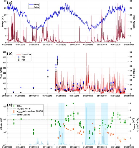
Turbidity values (Figure 2(b)) had a base level of approximately 20–30 NTU during periods of low salinity, reaching lower values only when salinity peaks occurred. Turbidity also presented relatively high variability, with peaks frequently exceeding 100 NTU. Both TSS and FSS had very similar positive correlation coefficients with turbidity, around 0.8 (linear) and 0.7 (rank). FSS accounted in general between 73% and 93% (percentiles 10 and 90) of the TSS concentrations, confirming that suspended sediments were mainly from mineral origin. The ratio between TSS and turbidity for the Río de la Plata Estuary was found to be in general 0.73 by Moreira et al. (2013), which is consistent with our field measurements.

Chl-a (Figure 2(c)) revealed a general seasonal cycle with higher concentrations in summer-autumn, reaching values of ∼10${}^2 \mu$ g/L, and minimums in winter of ∼10${}^0 \mu$ g/L. It can be observed that concentrations exceeded the WHO Alert Level II for recreational waters (24 μg/L) in at least one sample each year (see in Section 2.4 that cyanobacteria always dominate for this chl-a level).

The CDOM absorption coefficient at 443 nm ($a_{\text{CDOM}}(443)$), estimated from a linear relationship with CDOM fluorescence (see Section 2.1), tended to rise after a peak of the Santa Lucía river flow (see shaded periods in Figure 2(c)), while it was lowest by the end of the record, coinciding with practically null river flow and higher (maintained) salinity at the study site.

Time series revealed a dynamic estuarine environment with relatively high variability of turbidity. Turbidity presented a general increasing trend with significant wave height, being stronger for wave heights above 0.5 m (not shown). However, during field campaigns, which were performed with calm sea conditions, the turbidity range was considerably smaller, between 3 to 90 NTU (Table 1).

Table 1. Summary of field data collected at the sampling site when radiometric measurements were taken for the whole study period (2018–2020).

	Average	Median	25th prctile	75th prctile	Max	Min
Chl a (μg/L)	16.0	4.8	3.2	10.4	177.6	0.4
Turbidity (NTU)	31.4	28.2	18.6	39.8	90.4	2.7
TSS (mg/L)	14.6	11.2	8.7	17.3	74.5	3.9
FSS (mg/L)	11.4	8.6	6.5	13.8	68.4	2.5
$a_{\text{CDOM}}(443)$ (m^– 1)	1.813	1.807	1.428	2.331	3.083	0.499

Finally, the chl-a concentration was uncorrelated with all the other variables related to water colour (turbidity, TSS, FSS and CDOM), as given by their rank correlation coefficients: −0.2, 0.2, −0.02 and −0.03, respectively (p-value >0.05 for all variables).

3.2. Algorithms for chl-a estimation

3.2.1. Regional fits

Our regional fits for the chl-a indices presented in Section 2.3 (Figure 3 and Table 2) had high determination coefficient (R²) values ($\ge 0.96$) and root mean squared error (RMSE) between 5 and 7 μg/L for three of the indices: 3BI, NDCI, and SS(665). Their mean absolute (relative) errors were 3.7 μg/L for the NDCI, 4.8 μg/L (134%) for the 3BI, and 4.7 μg/L (76%) for the SS(665). Note that -SS(665) is considered in Figure 3 and hereon so that chl-a concentrations increase with the index. On the other hand, ${\mathrm{I}}_{\text{Drozd}}$ presented a considerably poorer performance, as the index seems to be insensitive to samples with lower turbidity levels, clearly overestimating their chl-a concentrations (Figure 3(c)). It is important to mention that the five data points with lowest turbidity (< 10 NTU) were not considered in the calibration of the ${\mathrm{I}}_{\text{Drozd}}$ index, but they were included to compute its performance metrics (Table 2).

Figure 3. Regional calibration of the four selected chl-a indices: (a) 3BI, (b) NDCI, (c) ${\mathrm{I}}_{\text{Drozd}},$ and (d) SS(665), considering S2-MSI bands. Colours indicate turbidity estimated from the NIR band centred at ∼740 nm. Error bars represent the standard deviation of chl-a measurements (note that in some cases it was not available). None of the quadratic fits (panels (b) and (d)) was able to estimate chl-a levels lower than 2 μg/L approximately.

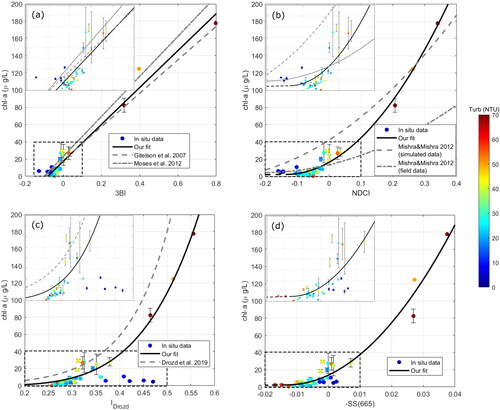
Table 2. Regional expressions for remote sensing estimation of chl-a concentrations ($[\text{chl} a]$) with the four selected indices. The number of data points (n), the root mean squared error (RMSE), and the determination coefficient (R²) of the fits are indicated (both computed in linear scale). (${}^{*}$) Expression is valid for $\text{ND}>-0.136.$ (**) Low turbidity samples were excluded from ${\mathrm{I}}_{\text{Drozd}}$ fit (see text). (***) Expression is valid for $\text{SS}(665)<0.0131$ (equivalent to $-\text{SS}(665)>-0.0131$).

Index (λ(nm))	Fit	n	RMSE (μg/L)	R2
$3\text{BI}$	$[\text{chl} a]=214.07(3\text{BI})+17.53$	43	6.4	0.96
$\text{NDCI}$	$[\text{chl} a]=762.6{(\text{NDCI})}^2+207.4(\text{NDCI})+16.4$ (${}^{*}$)	43	4.9	0.98
${\mathrm{I}}_{\text{Drozd}}$	$[\text{chl} a]=3154.7{({\mathrm{I}}_{\text{Drozd}})}^{4.86}$	38(**)	17.8	0.77
$\text{SS}(665)$	$[\text{chl} a]=66067{(\text{SS}(665))}^2-1726.9(\text{SS}(665))+13.65$ (***)	43	7.2	0.96

The obtained algorithms (Table 2) were calibrated for chl-a concentrations between 0.4 and 180 μg/L (maximum and minimum values in Table 1), although most of the samples presented lower chl-a concentrations, between 3 and 10 μg/L (percentiles 25th and 75th in Table 1). Moreover, the turbidity levels for the dataset were between 3 and 90 NTU, although they were mostly in the range 20–40 NTU, while CDOM absorption at 443 nm was approximately between 0.5 and 3.1 m^{– 1}, but mostly in the range 1.4–2.3 m^{– 1}.

Chl-a indices presented some correlations with measured CDOM and turbidity. The following correlation coefficients were obtained with CDOM: 0.45 (linear) and 0.49 (rank) for NDCI, 0.59 and 0.53 for 3BI, −0.51 and −0.37 for ${\mathrm{I}}_{\text{Drozd}},$ and 0.20 and 0.08 for -SS(665). The SS(665) index had the lowest (and negligible) correlation with CDOM, while it was stronger for 3BI. The correlation coefficients with turbidity were as follows: 0.45 (linear) and 0.42 (rank) for NDCI, 0.46 and 0.49 for 3BI, −0.54 and −0.77 for ${\mathrm{I}}_{\text{Drozd}},$ and −0.38 and −0.52 for -SS(665). It can be observed that all indices showed some relationship to turbidity, being stronger (and negative) for ${\mathrm{I}}_{\text{Drozd}},$ and similar (in absolute value) among the other indices. These correlations among chl-a indices and water-colour related variables are not consistent wit results in Section 3.1, where CDOM and turbidity were uncorrelated with extracted chl-a. This implies that remote sensing of chl-a may be affected by CDOM and turbidity levels, which is further discussed in Section 3.3.

3.2.2. Comparison with previous algorithms

Our results were compared to algorithms previously proposed by other authors for the same chl-a indices, considering the regions and range of constituents related to water colour of these previous applications.

The index ${\mathrm{I}}_{\text{Drozd}}$ was calibrated for a reservoir (Salto Grande, located upstream of the study region) by Drozd et al. (2020), considering S2-MSI bands. They proposed a linear fit between the ${\mathrm{I}}_{\text{Drozd}}$ and logarithmic chl-a concentrations, which tended to overestimate our measured chl-a levels for most samples (Figure 3(c)). This overestimation could be caused by different characteristics of the optically active constituents in both datasets. Their algorithm was optimized for relatively high chl-a levels (mean concentration of 278 μg/L), with predominance of cyanobacteria in most cases. In our dataset, on the other hand, while cyanobacteria dominated all samples with chl-a above 15 μg/L, most of our measurements had lower concentrations (Table 1). Moreover, although Drozd et al. (2020) reported a wide range of TSS concentrations (5–467 mg/L), TSS was positively correlated with chl-a in the Salto Grande reservoir, suggesting that the phytoplankton was an important component of the suspended particulate matter, which was not found to be true for the Río de la Plata.

The NDCI was proposed for MERIS satellite bands in the work of Mishra and Mishra (2012), considering both simulated and field data for several study regions: the Mississippi River Delta, Chesapeake Bay and Delaware Bay, the Mississippi Sound and Mobile Bay. They proposed an empirical quadratic fit, based on the best statistical performance among different linear and non-linear trends. The algorithm obtained for their simulated dataset tended to overestimate our measurements, while their calibration with field data tended to overestimate our lower chl-a concentrations and underestimate the higher ones (Figure 3(b)). Regarding the concentrations of optically active water constituents, the chl-a range in Mishra and Mishra (2012) was similar to our dataset: from 0 to 60 μg/L for their simulated data, and from 0.9 to 28.1 μg/L for their field data; the variability in the CDOM absorption coefficient covered the range found in our study region (from 0.05 to 5 m^{– 1} at 440 nm); and the range of suspended sediment concentration was somewhat narrower (2–10 mg/L of inorganic suspended sediments). Despite the apparent similarities in the ranges of water constituents, our regional fit gave quite different calibration parameters, calling the attention on the importance of algorithm validation in optically complex waters.

Our linear regional fit for the 3BI closely agreed with previous ones proposed for MERIS bands by Gitelson et al. (2007); Moses et al. (2012; Figure 3(a)) for the Chesapeake Bay and the Azov Sea, respectively, suggesting that the 3BI may be more robust for different water bodies. Their chl-a ranges were 9.0–77.4 μg/L (Gitelson et al. 2007) and 1.09–107.82 (Moses et al. 2009); CDOM absorption at 440 nm was reported between 0.20 to 2.50 m^{– 1} and TSS between 7 and 65 mg/L in Gitelson et al. (2007). It is worth highlighting that if the phytoplankton absorption coefficient is assumed directly proportional to chl-a levels, a linear relationship is consistent with the semi-analytical development of the 3BI (Le et al. 2011).

Finally, SS indices have been widely used in the literature, such as the fluorescence line height (FLH) (Gower 1980; Gower et al. 1999), the floating algal index (FAI) (Hu 2009), the maximum chlorophyll index (MCI) (Gower et al. 2005, 2008), and the colour index-based algorithm (CIA) (Hu et al. 2012). The FLH is centred at the chl-a fluorescence peak, around 681 nm, which is not available in S2-MSI, while FAI, MCI and CIA can be computed for S2-MSI bands, centered at the NIR (865 nm), red-edge (705 nm), and green bands (560 nm), respectively. The same satellite band set used to estimate FLH was used to develop a cyanobacteria-related chl-a index (CI) (Wynne et al. 2008). Lunetta et al. (2015) used CI, but incorporating a relative peak centred at 665 nm, with the linear baseline computed from 620 and 681 nm, as an exclusion criterion to determine cyanobacteria presence. Matthews et al. (2012) proposed the maximum peak height (MPH) algorithm to estimate chl-a, defining MPH as the dominant peak across the red and NIR MERIS bands centred at 681, 709 and 753 nm, using a baseline between 664 and 885 nm. In this work, however, the SS index that had higher correlations with measured chl-a concentration was centred at the red band (665 nm), with the baseline between the green (560 nm) and red-edge bands (705 nm) (see Appendix A, the Supplemental material). To the best of the authors knowledge, this index has not been previously reported in the literature, probably because many of the works used satellite bands that are not available in S2-MSI. The expression that gave statistically best results for the study region was a quadratic fit (Figure 3(d)).

3.2.3. Relation of S2-MSI indices to water reflectance features

The four chl-a indices considered in this work have two bands in common: the red (665 nm) and red-edge (705 nm). The importance of a band centred at slightly over 700 nm for the detection of phytoplankton blooms was already remarked by Gitelson (1992); Gower et al. (2008). The water-leaving reflectance (${\rho }_{\mathrm{w}}(\lambda )$) can be related to the inherent optical properties (IOPs) of the water (and its constituents) through the absorption coefficient ($a(\lambda )$) and the backscattering coefficient ($b_b(\lambda )$), as ${\rho }_{\mathrm{w}}(\lambda )=f\left\{b_b(\lambda )/[a(\lambda )+b_b(\lambda )]\right\}$ (Gordon et al. 1988; Lee et al. 2002). Hence, the absorption peak of chl-a, centred at 675 nm, generates a trough in ${\rho }_{\mathrm{w}},$ while a peak is observed near 700 nm due to the backscattering of (phytoplankton) particles in combination with the rapid rise in water absorption that occurs towards the NIR region (Gitelson et al. 1999). These features can be captured by the red (at 665 nm) and red-edge (at 705 nm) bands of S2-MSI. In sediment-rich waters, the backscattering of sediments further increases reflectance in the red-NIR range; however, the narrow-band absorption feature of chl-a can be detected by comparison of the red and red-edge bands (Gower et al. 2008), due to the smooth spectral features of sediments IOPs. Regarding the potential effects of chl-a fluorescence induced by sunlight, which is also a narrow-band feature but peaks at about 685 nm, it should not greatly affect reflectance at S2-MSI bands, and furthermore, for cyanobacteria dominance (found for higher chl-a levels at the study site, see Section 2.4), the effect would be reduced as cyanobacteria produce low chl-a fluorescence (Stumpf et al. 2016). It is worth highlighting that phycocyanin, which is a marker pigment of freshwater cyanobacteria, strongly absorbs around 620 nm, but unfortunately cannot be detected by S2-MSI bands (Stumpf et al. 2016).

Although the -SS(665) index has not been previously applied considering bands similar to those of S2-MSI as in the case of other chl-a indices, the good results obtained for our study region are supported by the previous observations regarding spectral absorption and backscattering features. Findings in Gitelson et al. (1999) also support the good performance of this index, as they revealed that the red trough is much less sensitive to variations in phytoplankton densities than the magnitudes of the green and red-edge peaks of the reflectance spectra, regardless of the phytoplankton species. Nevertheless, the obtained algorithm should be further tested as more field data is collected for the estuary.

3.3. Mapping chl-a

3.3.1. Results with regional algorithms

The regional algorithms obtained in Section 3.2 allowed us to retrieve chl-a maps for the study region from the available S2 images. Two dates were selected as examples, December 2 and 17 of 2019 (Figures 4 and 5), to summarize results that were observed in general for the whole study period (2018–2021). Turbidity presented high spatial variability in the region, varying one or two orders of magnitude, with the turbidity maximum often present in the area, and frequently exceeding 100 NTU (panels (f)). The 3BI and NDCI (panels (a-b)) seemed to replicate the spatial patterns of turbidity, estimating higher chl-a concentrations for more turbid waters. On the other hand, ${\mathrm{I}}_{\text{Drozd}}$ and the -SS(665) index (panels (c-d)) presented opposite trends than 3BI and NDCI, i.e. estimating higher chl-a concentrations for less turbid (clearer) waters. These trends are consistent with the correlations between the chl-a indices and measured turbidity levels described in Section 3.2.1. The considerable overestimation of chl-a levels by ${\mathrm{I}}_{\text{Drozd}}$ in clear waters, which was already observed for the calibration dataset (Figure 3(c)), can be clearly seen in the example of Figure 4(c), discouraging the use of this index for the study region.

Figure 4. Examples of chl-a retrievals at the study region for December 2, 2019: (a) with 3BI, (b) with NDCI, (c) with ${\mathrm{I}}_{\text{Drozd}},$ and (d) with SS(665); (e) the uncertainty was computed pixel-by-pixel as the interquartile range between estimations (a) to (c) relative to their median result; (f) turbidity levels were estimated from the NIR band centred at 740 nm.

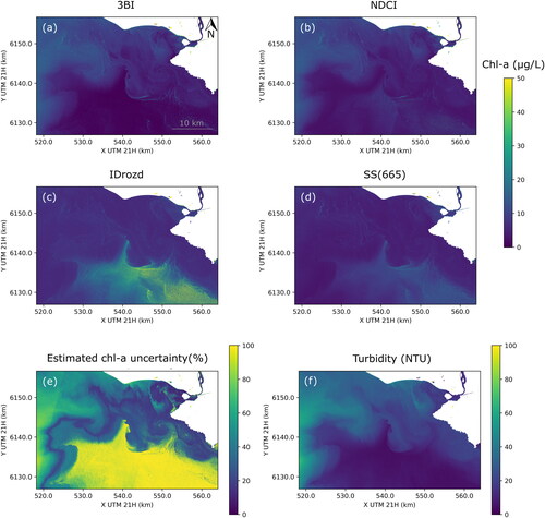
Figure 5. Same as Figure 4 but for December 17, 2019.

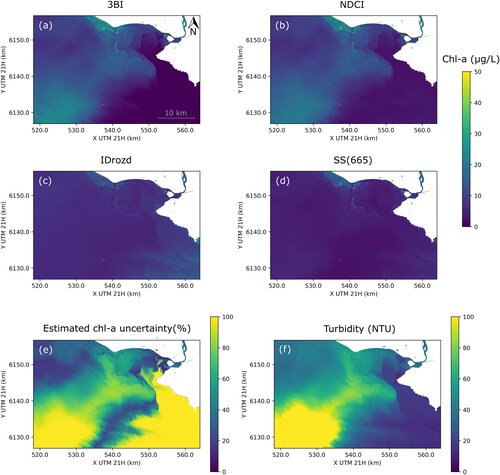
The variability within the chl-a estimations was computed as the interquartile range among the four indices relative to their median in a pixel-by-pixel basis (panels (e)). It was observed that their difference was lower in zones where turbidity was within the 25th and 75th percentiles obtained during field campaigns, while was higher in the turbidity maximum (e.g. SW of Figure 5(e)) and in clear waters (e.g. S of Figure 4(e) and SE of Figure 5(e)). Regarding differences with measured chl-a concentrations, -SS(665) seemed to better discriminate the samples with lower chl-a than the other indices (Figure 3(d)), at least for the ranges of turbidity and CDOM registered during field campaigns. For instance, chl-a from samples collected in December 2, 2019, was on average 4.74 μg/L, which was better estimated by -SS(665) in this case (Figure 4(d)). On the other hand, as chl-a concentrations increased, all indices retrieved more similar results (lower relative differences among retrievals). For example, in December 17, 2019, chl-a between 20.7 and 30.4 μg/L were measured during the field campaign, and all indices estimated chl-a levels around 30 μg/L in the north coast near the sampling site (Figure 5(a–d)), clearly reducing the relative difference between estimations in that area (Figure 5(e)).

3.3.2. Implications for monitoring threshold levels

Results presented in Section 3.3.1 revealed limitations in the application of indices to monitor chl-a thresholds in the coast of the Río de la Plata, as the use of regionally calibrated algorithms, with similar performances (Table 2), gave quite different retrievals as optical properties diverged from the ones registered during field campaigns (Figures 4 and 5). As an example, the threshold maps for the level of 10 μg/L, associated to low potential health risks for recreational waters (Section 2.4), are shown in Figure 6. We considered two of the regional algorithms (using 3BI and -SS(665)) for the same dates presented in Figures 4 and 5. It can be observed that the regions where both indices agree (black pixels in Figure 6) are significantly smaller than the area retrieved if only one index is considered (red pixels in Figure 6), which is practically most of the study region. It is worth mentioning that results were very similar if the regional algorithm for the NDCI was used instead of the one for the 3BI, while ${\mathrm{I}}_{\text{Drozd}}$ was not considered due to its poor performance in clearer waters.

Figure 6. Chl-a threshold maps retrieved at the study region from S2-MSI images for the level of 10 μg/L, matching the two dates in Figures 4 and 5: (a) December 2 and (b) December 17, 2019. The regional algorithms for 3BI and SS(665) were used, and the highlighted areas in both panels indicate where none, one, or two of the indices estimated chl-a level above 10 μg/L.

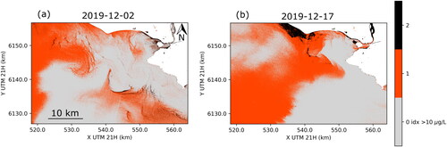
This disagreement between algorithms emerges due to the highly variable levels of optically active constituents, being especially evident for turbidity, which can be considered as a proxy for (mainly inorganic) suspended sediments (Section 3.1). As mentioned earlier, all chl-a indices presented statistically significant correlations with in-situ measured turbidity (Section 3.2.1). On top of this, the levels captured during field campaigns, which were performed with calm weather conditions, were likely limited considering the variability that can be found in the estuary. For instance, turbidity was below 100 NTU during field visits (Table 1), although this value was reached approximately weekly at the moored station (Figure 2(b)), matching the occurrence of storms, when field campaigns were less feasible. Furthermore, values around 100 NTU are typically exceeded in different zones of the Rio de la Plata (Dogliotti et al. 2016), often nearby the study site (e.g. Figure 5(f)).

Despite the previous limitations, it was noted that the simultaneous application of two indices (e.g. Figure 6) that presented opposite trends regarding turbidity could be useful for detecting chl-a threshold levels of interest for monitoring potential cyanobacterial blooms. The opposite trends found between the 3BI or NDCI and the -SS(665) or ${\mathrm{I}}_{\text{Drozd}}$ algorithms were already described in Section 3.3.1 in terms of variations in turbidity levels. Moreover, they were further explored with a simplified set of synthetic spectra obtained with average coastal IOPs, as described in Appendix B (the Supplemental material). Results confirmed the general trends previously observed for the chl-a algorithms (e.g. in Figures 4 and 5), associating them to TSS and CDOM variability. Although the four indices presented limitations to retrieve chl-a in environments with highly variable TSS and CDOM concentrations, -SS(665) showed a more steady behaviour for chl-a around $\sim 10 \mu$ g/L or lower, while 3BI seemed better for higher chl-a concentrations (Appendix B, the Supplemental material). NDCI presented a similar behaviour than 3BI, but the latter was preferred for further implementations in this study due to the similarity of our regional fit to previously proposed algorithms (Section 3.2.2), suggesting a more robust behaviour in optically complex waters.

3.3.3. Example of monitoring application

We used the regional algorithm obtained for -SS(665) in simultaneous with the one for 3BI to obtain chl-a threshold maps for the coastal region of the Río de la Plata estuary for the whole study period (February 2018 to April 2020), which are included in Appendix C (the Supplemental material).

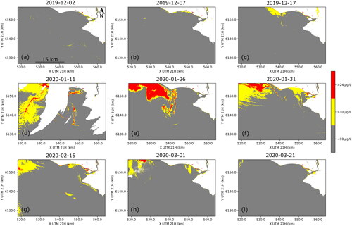
In this Section, we show the period from December 2019 to March 2020 as an example application of the proposed method for bloom monitoring. This period was selected considering that the turbidity and salinity dynamics at the study site (Figure 2(a)) were especially challenging for chl-a remote sensing, as the presence of both turbid and clear water masses limited the performance of each index individually. Near true colour composites of S2-MSI images are shown in Appendix C (the Supplemental material) as a reference to qualitatively observe the variation in water masses. In a temporal sequence of maps, we followed the extension of the two selected chl-a threshold levels (Figure 7). In the beginning of December 2019, areas with chl-a above 10 μg/L observed along the north coast increased by December 17, when also patches with chl-a concentrations above 24 μg/L were detected. By January 2020, a large bloom (chl-a $>24 \mu$ g/L) covered the study area. The peak of the bloom occurred in mid to late January 2020. On January 17, chl-a concentrations of up to 38 μg/L were measured at the sampling site, with cyanobacterial biovolume of 5 mm³/L. Two days previous to February 15, persistent NE winds (∼10 m/s) occurred in the study region, which probably contributed to move the bloom off from the coast (Figure 7(g)). By the end of March, the bloom size decreased and the levels of chl-a were low ($<10 \mu$ g/L). This bloom event corresponded to a cyanobacterial bloom, as it was confirmed in the field campaigns. Furthermore, for chl-a concentrations above 24 μg/L, it is expected that cyanobacteria dominate the phytoplankton composition at the study site (see Section 2.4).

Figure 7. Sequence of chl-a threshold maps for the summer 2019–2020 obtained using S2-MSI imagery. Highlighted areas indicate where both indices 3BI and -SS(665) exceeded chl-a levels of 10 and 24 μg/L. Three consecutive smoothing (median) filters of 7, 5, and 3 pixels were applied to these maps.

Identification and location of cyanobacterial biomass accumulations, not visible from the coast, is important in estuaries such as the Río de la Plata. It is a highly dynamic ecosystem, resulting in large variability of cyanobacterial biomass in time and space, which imposes an important challenge for monitoring (Sathicq et al. 2014). Moreover, persistent winds may transport cyanobacterial populations to the coast, potentially impacting recreational areas and drinking water intakes within relatively short time frames (Sathicq et al. 2014). Our approach allowed to successfully follow the evolution of a cyanobacterial bloom by identifying levels of chl-a that are regularly used as indicators of risk of exposure to toxic cyanobacteria, proving to be a useful tool to complement already existing monitoring programs that are based on in-situ observations (Pirez et al. 2013; Aubriot et al. 2020). Furthermore, it has the potential to be incorporated into early alert systems, as 10 μg/L threshold areas were observed (e.g. in early December 2019), before higher chl-a levels (24 μg/L) were reached (e.g. in January 2020).

4. Conclusions

This study presents the first evaluation of chl-a estimations from high spatial-resolution satellite sensors (S2-MSI) in the Río de la Plata estuary, using a two-year long data set that covered a wide range of environmental conditions. Different types of band-combination indices were explored using in-situ radiometric data and chl-a measurements collected in the intermediate zone of the estuary, close to its northern coast. Regional algorithms were obtained for the study site and compared to previous ones when available. For the 3BI index (Dall’Olmo et al. 2003), the regional fit closely matched algorithms previously applied to other water bodies (Gitelson et al. 2007; Moses et al. 2012). On the other hand, previous calibrations of the NDCI (Mishra and Mishra 2012) and ${\mathrm{I}}_{\text{Drozd}}$ (Drozd et al. 2020) had poor performances in the Río de la Plata, highlighting the importance of local data collection for regional testing and validation of remote sensing products. This work also proposes the use of the spectral shape centred at red band of S2-MSI (-SS(665)). Although similar to other SS indices (Gower et al. 2005; Wynne et al. 2008; Hu 2009; Matthews et al. 2012), to the best of our knowledge the -SS(665) has not been previously applied considering S2-MSI bands, with a linear baseline between the green and red-edge bands (at 560 and 705 nm, respectively). A quadratic algorithm was fitted for -SS(665) at the study region, which better discriminated samples with low chl-a than the algorithms obtained for 3BI, NDCI and ${\mathrm{I}}_{\text{Drozd}}.$ The robustness of the regional fit should be further tested as more field data is collected for the estuary.

When applied to S2-MSI imagery, it was found that the four selected indices presented limitations to retrieve chl-a with highly variable turbidity levels. The spatial variability of turbidity found in the Río de la Plata is difficult to capture during routine field campaigns, partly because of their design: relatively close to the coast and during calm weather conditions. Although satellite imagery is a powerful tool to precisely capture the spatial variability of water quality parameters, covering large areas that are difficult or costly for monitoring programs, their information can be misleading if it is not properly analyzed in terms of the variations of all optically active constituents. To overcome the challenges imposed by the high variability of turbidity levels (mainly associated to inorganic suspended sediments) on chl-a retrievals, we proposed the simultaneous application of two algorithms, based on 3BI and -SS(665), to monitor chl-a threshold levels that are of interest for risk exposure when cyanobacteria dominate. This work successfully follows the evolution of chl-a thresholds on a large spatial scale in a dynamic environment. The proposed approach can be easily implemented in monitoring efforts and protocols, providing a cost-effective way to significantly increases the frequency and spatial extent of observations, being of potential great interest for policy makers, tourism managers and fisheries.

Acknowledgments

The authors also want to thank the assistance of Matías González and Rodrigo Mosquera during field measurements, and the assistance of Katherine Bombi in laboratory analyses. Part of the data used in this work was collected during field campaigns in the frame of an outreach project for UTE.

Disclosure statement

No potential conflict of interest was reported by the authors.

Additional information

Funding

This manuscript was possible thanks to the support of the Sistema Nacional de Investigadores (National Researchers System, Uruguay), the Project FMV-1-2017-1-136098 from Agencia Nacional de Investigación e Innovación (ANII, National Research and Innovation Agency, Uruguay), the fund for scientific equipment from Comisión Sectorial de Investigación Científica (CSIC, Scientific Research Committee) of the Universidad de la República, Uruguay, the Project ID24 (2017) from CSIC and UTE (National Electric Administration of Uruguay), and the fellowship for graduate studies granted to F. Maciel by the Comisión Acadmémica de Posgrado (Academic Graduate Committee) of the Universidad de la República, Uruguay.

References

- Armstrong RA, Gilbes F, Guerrero R, Lasta C, Benavidez H, Mianzan H. 2004. Validation of SeaWiFS-derived chlorophyll for the Rio de la Plata Estuary and adjacent waters. Int J Remote Sensing. 25(7–8):1501–1505.
- Aubriot L, Zabaleta B, Bordet F, Sienra D, Risso J, Achkar M, Somma A. 2020. Assessing the origin of a massive cyanobacterial bloom in the Río de la Plata (2019): towards an early warning system. Water Res. 181:115944.
- Borfecchia F, Micheli C, Cibic T, Pignatelli V, De Cecco L, Consalvi N, Caroppo C, Rubino F, Di Poi E, Kralj M, et al. 2019. Multispectral data by the new generation of high-resolution satellite sensors for mapping phytoplankton blooms in the Mar Piccolo of Taranto (Ionian Sea, southern Italy). European J Remote Sens. 52(1):400–418.
- Bramich J, Bolch CJS, Fischer A. 2021. Improved red-edge chlorophyll-a detection for Sentinel 2. Ecol Indic. 120:106876.
- Cannizzaro JP, Barnes BB, Hu C, Corcoran AA, Hubbard KA, Muhlbach E, Sharp WC, Brand LE, Kelble CR. 2019. Remote detection of cyanobacteria blooms in an optically shallow subtropical lagoonal estuary using MODIS data. Remote Sens Environ. 231:111227.
- Carreto JI, Montoya N, Akselman R, Carignan MO, Silva RI, Cucchi Colleoni D. A. 2008. Algal pigment patterns and phytoplankton assemblages in different water masses of the Río de la Plata maritime front. Contin Shelf Resear. 28(13):1589–1606.
- Chorus I, Welker M. 2021. Exposure to cyanotoxins: understanding it and short-term interventions to prevent it. In: I. Chorus and M. Welker, editors. Toxic cyanobacteria in water. A guide to their public health consequences, monitoring and management. 2nd ed., Chap. 5. CRC Press, Boca Raton (FL), on behalf of the World Health Organization, Geneva; p. 295–400.
- Coronado-Franco KV, Selvaraj JJ, Mancera Pineda JE. 2018. Algal blooms detection in Colombian Caribbean Sea using MODIS imagery. Mar Pollut Bull. 133:791–798.
- Dall’Olmo G, Gitelson AA, Rundquist DC. 2003. Towards a unified approach for remote estimation of chlorophyll-a in both terrestrial vegetation and turbid productive waters. Geophys Res Lett. 30(18):1938.
- Dall’Olmo G, Gitelson AA, Rundquist DC, Leavitt B, Barrow T, Holz JC. 2005. Assessing the potential of SeaWiFS and MODIS for estimating chlorophyll concentration in turbid productive waters using red and near-infrared bands. Remote Sens Environ. 96(2):176–187.
- Dogliotti AI, Gossn JI, Gonzalez C, Yema L, Sanchez ML, O’Farrell I. 2021. Evaluation of multi- and hyper- spectral chl-a algorithms in the Río de la Plata turbid waters during a cyanobacteria bloom. In 2021 IEEE International Geoscience and Remote Sensing Symposium IGARSS, Brussels, Belgium; p. 7442–7445. IEEE.
- Dogliotti AI, Ruddick K, Guerrero R. 2016. Seasonal and inter-annual turbidity variability in the Río de la Plata from 15 years of MODIS: el Niño dilution effect. Estuarine, Coastal and Shelf Science. 182:27–39.
- Drozd A, de Tezanos Pinto P, Fernández V, Bazzalo M, Bordet F, Ibañez G. 2020. Hyperspectral remote sensing monitoring of cyanobacteria blooms in a large South American reservoir: high- and medium-spatial resolution satellite algorithm simulation. Mar Freshwater Res. 71(5):593–605.
- Fossati M, Cayocca F, Piedra-Cueva I. 2014. Fine sediment dynamics in the Río de la Plata. Adv Geosci. 39:75–80.
- Framiñan MB, Brown OB. 1996. Study of the Rio de la Plata turbidity front, Part I: spatial and temporal distribution. Continen Shelf Resear. 16(10):1259–1282.
- García-Alonso J, Lercari D, Defeo O. 2019. Río de la Plata: a neotropical Estuarine system. In: E. Wolanski, J. W. Day, M. Elliott, and R. Ramachandran, editors. Coasts and Estuaries. Chap. 3. Amsterdam: Elsevier; p. 45–56.
- Garcia CAE, Garcia VMT. 2008. Variability of chlorophyll-a from ocean color images in the La Plata continental shelf region. Continen Shelf Resear. 28(13):1568–1578.
- Garcia VMT, Signorini S, Garcia CAE, McClain CR. 2006. Empirical and semi-analytical chlorophyll algorithms in the southwestern Atlantic coastal region (25–40 S and 60–45 W). Int J Remote Sens. 27(8):1539–1562.
- Gernez P, Doxaran D, Barille L. 2017. Shellfish aquaculture from space: potential of Sentinel 2 to monitor tide-driven changes in Turbidity, chlorophyll concentration and oyster physiological response at the scale of an Oyster Farm. Front Mar Sci. 4: 137
- Gholizadeh MH, Melesse AM, Reddi L. 2016. A comprehensive review on water quality parameters estimation using remote sensing techniques. Sensors. 16(8):1298.
- Giannini MFC, Garcia CAE, Tavano VM, Ciotti AM. 2013. Effects of low-salinity and high-turbidity waters on empirical ocean colour algorithms: an example for Southwestern Atlantic waters. Continen Shelf Resear. 59:84–96.
- Giannuzzi L, Carvajal G, Corradini MG, Araujo-Andrade C, Echenique R, Andrinolo D. 2012. Occurrence of toxic cyanobacterial blooms in Río de la Plata Estuary, Argentina: field study and data analysis. J Toxicol. 2012:1–15.
- Gitelson AA. 1992. The peak near 700 nm on radiance spectra of algae and water: relationships of its magnitude and position with chlorophyll concentration. Inter J Remote Sens. 13(17):3367–3373.
- Gitelson AA, Schalles JF, Hladik CM. 2007. Remote chlorophyll-a retrieval in turbid, productive estuaries: chesapeake Bay case study. Remote Sens Environ. 109(4):464–472.
- Gitelson AA, Schalles JF, Rundquist D. C, Schiebe YZ, Yacobi FR. 1999. Comparative reflectance properties of algal cultures with manipulated densities. J Appl Phycol. 11(4):345–354.
- Gohin F, Lampert L, Guillaud JF, Herbland A, Nézan E. 2003. Satellite and in situ observations of a late winter phytoplankton bloom, in the northern Bay of Biscay. Continen Shelf Resear. 23(11–13):1117–1141.
- Gons HJ, Rijkeboer M, Ruddick KG. 2002. A chlorophyll-retrieval algorithm for satellite imagery (Medium Resolution Imaging Spectrometer) of inland and coastal waters. J Plankton Research. 24(9):947–951.
- Gordon HR, Brown OB, Evans RH, Brown JW, Smith RC, Baker KS, Clark D. K. 1988. A semianalytic radiance model of Ocean Color. J Geophys Res. 93(D9):10909–10924.
- Gower J, King S, Borstad G, Brown L. 2005. Detection of intense plankton blooms using the 709 nm band of the MERIS imaging spectrometer. Inter J Remote Sens. 26(9):2005–2012.
- Gower J, King S, Borstad G, Brown L. 2008. The importance of a band at 709 nm for interpreting water-leaving spectral radiance. Can. J. Remote Sens. 34(3):287–295.
- Gower JFR. 1980. Observations of in situ fluorescence of chlorophyll-a in Saanich Inlet. Boundary-Layer Meteorol. 18(3):235–245.
- Gower JFR, R, Doerffer, GA, Borstad. 1999. Interpretation of the 685 nm peak in water-leaving radiance spectra in terms of fluorescence, absorption and scattering, and its observation by MERIS. Inter J Remote Sens. 20(9):1771–1786.
- Hillebrand H, Durselen C, Kirschtel D, Pollingher U, Zohary T. 1999. Biovolume calculation for pelagic and benthic microalgae. J. Phycol. 35(2):403–424.
- Hu C. 2009. A novel ocean color index to detect floating algae in the global oceans. Remote Sens Environ. 113(10):2118–2129.
- Hu C, Lee Z, Franz B. 2012. Chlorophyll a algorithms for oligotrophic oceans: a novel approach based on three-band reflectance difference. J Geophys Resear. 117: c1011.
- Huisman J, Codd GA, Paerl HW, Ibelings BW, Verspagen JMH, Visser PM. 2018. Cyanobacterial blooms. Nat Rev Microbiol. 16(8):471–483.
- Huret M, Dadou I, Dumas F, Lazure P, Garcon V. 2005. Coupling physical and biogeochemical processes in the Río de la Plata plume. Continental Shelf Research. 25(5–6):629–653.
- ISO-10260. 1992. Water quality measurement of biochemical parameters: spectrophotometric determination of chlorophyll-a concentration. Standard 10260. Geneva, Switzerland: international Organization for Standardization.
- Jaureguizar AJ, Solari A, Cortés F, Milessi AC, Militelli MI, Camiolo MD, Clara ML, García M. 2016. Fish diversity in the Río de la Plata and adjacent waters: an overview of environmental influences on its spatial and temporal structure. J Fish Biol. 89(1):569–600.
- Kahru M, Elmgren R. 2014. Multidecadal time series of satellite-detected accumulations of cyanobacteria in the Baltic Sea. Biogeosciences. 11(13):3619–3633.
- Khan RM, Salehi B, Mahdianpari M, Mohammadimanesh F, Mountrakis G, Quackenbush LJ. 2021. A meta-analysis on Harmful Algal Bloom (HAB) detection and monitoring: a remote sensing perspective. Remote Sens. 13(21):4347.
- Kruk C, Martínez A, Martínez de la Escalera G, Trinchin R, Manta G, Segura AM, Piccini C, Brena B, Yannicelli B, Fabiano G, et al. 2021. Rapid freshwater discharge on the coastal ocean as a mean of long distance spreading of an unprecedented toxic cyanobacteria bloom. Sci Total Environ. 754:142362.
- Le C, Li Y, Zha Y, Sun D, Huang C, Zhang H. 2011. Remote estimation of chlorophyll a in optically complex waters based on optical classification. Remote Sensing of Environment. 115(2):725–737.
- Lee Z, Carder KL, Arnone RA. 2002. Deriving inherent optical properties from water color: a multiband quasi-analytical algorithm for optically deep waters. Appl Opt. 41(27):5755–5772.
- Lunetta RS, Schaeffer BA, Stumpf RP, Keith D, Jacobs SA, Murphy MS. 2015. Evaluation of cyanobacteria cell count detection derived from MERIS imagery across the eastern USA. Remote Sens Environ. 157:24–34.
- Machado I, Barreiro M, Calliari D. 2013. Variability of chlorophyll-a in the Southwestern Atlantic from satellite images: seasonal cycle and ENSO influences. Continen Shelf Resear. 53:102–109.
- Maciel FP, Pedocchi F. 2022. Evaluation of ACOLITE atmospheric correction methods for Landsat-8 and Sentinel-2 in the Río de la Plata turbid coastal waters. Inter J Remote Sens. 43(1):215–240.
- Maciel FP, Santoro PE, Pedocchi F. 2021. Spatio-temporal dynamics of the Río de la Plata turbidity front; combining remote sensing with in-situ measurements and numerical modeling. Continen Shelf Resear. 213:104301.
- Mannino A, Novak MG, Nelson N. B, Belz M, Berthon J-F, Blough N. V, Boss E. 2019. Measurement protocol of absorption by chromophoric dissolved organic matter (CDOM) and other dissolved materials. In: A. Mannino and M. G. Novak, editors. Inherent Optical Property Measurements and Protocols: absorption Coefficient. Darmouth, NS, Canada: IOCCG.
- Martínez de la Escalera G, Segura AM, Kruk C, Ghattas B, Cohan FM, Iriarte A, Piccini C. 2022. Genotyping and multivariate regression trees reveal ecological diversification within the microcystis aeruginosa complex along a wide environmental gradient. Appl Environ Microbiol. 88(3): e01475–21
- Matthews MW. 2011. A current review of empirical procedures of remote sensing in inland and near-coastal transitional waters. Inter J Remote Sens. 32(21):6855–6899.
- Matthews MW, Bernard S, Robertson L. 2012. An algorithm for detecting trophic status (chlorophyll-a), cyanobacterial-dominance, surface scums and floating vegetation in inland and coastal waters. Remote Sens Environ. 124:637–652.
- Matthews MW, Odermatt D. 2015. Improved algorithm for routine monitoring of cyanobacteria and eutrophication in inland and near-coastal waters. Remote Sens Environ. 156:374–382.
- Menéndez M. 2017. Determinación de sólidos suspendidos totales, fijos y volátiles en aguas naturales y efluentes líquidos. Método gravimétrico. Manual 1020UY. Uruguay: Dirección Nacional de Medio Ambiente.
- Mishra S, Mishra D. R. 2012. Normalized difference chlorophyll index: a novel model for remote estimation of chlorophyll-a concentration in turbid productive waters. Remote Sens Environ. 117:394–406.
- Mobley CD. 1999. Estimation of the remote-sensing reflectance from above-surface measurements. Appl Opt. 38(36):7442–7455.
- Moreira D, Simionato CG, Gohin F, Cayocca F, Luz M, Tejedor C. 2013. Suspended matter mean distribution and seasonal cycle in the Río de la Plata estuary and the adjacent shelf from ocean color satellite (MODIS) and in-situ observations. Continen Shelf Resear. 68:51–66.
- Morel A, Prieur L. 1977. Analysis of variations in ocean color. Limnol Oceanogr. 22(4):709–722.
- Moses W, Gitelson A, Berdnikov S, Povazhnyy V. 2009. Satellite estimation of chlorophyll-a concentration using the red and NIR bands of MERIS—The Azov Sea case study. IEEE Geosci Remote Sens Lett. 6(4):845–849.
- Moses WJ, Gitelson AA, Berdnikov S, Saprygin V, Povazhnyi V. 2012. Operational MERIS-based NIR-red algorithms for estimating chlorophyll-a concentrations in coastal waters—The Azov Sea case study. Remote Sens Environ. 121:118–124.
- Nagy GJ, Gómez-Erache M, López CH, Perdomo AC. 2002. Distribution patterns of nutrients and symptoms of eutrophication in the Rio de la Plata River Estuary system. In: E. Orive, M. Elliott, and V.N. de Jonge, editors. Nutrients and Eutrophication in Estuaries and Coastal Waters. Developments in Hydrobiology. Vol. 164. p. 125–139. Dordrecht: Springer.
- O’Neil JM, Davis TW, Burford MA, Gobler CJ. 2012. The rise of harmful cyanobacteria blooms: the potential roles of eutrophication and climate change. Harmful Algae. 14:313–334.
- Pahlevan N, Smith B, Alikas K, Anstee J, Barbosa C, Binding C, Bresciani M, Cremella B, Giardino C, Gurlin D, et al. 2022. Simultaneous retrieval of selected optical water quality indicators from Landsat-8, Sentinel-2, and Sentinel-3. Remote Sens Environ. 270:112860.
- Pahlevan N, Smith B, Schalles J, Binding C, Cao Z, Ma R, Alikas K, Kangro K, Gurlin D, Hà N, et al. 2020. Seamless retrievals of chlorophyll-a from Sentinel-2 (MSI) and Sentinel-3 (OLCI) in inland and coastal waters: a machine-learning approach. Remote Sens Environ. 240:111604.
- Pilotto LS, Douglas RM, Burch MD, Cameron S, Beers M, Rouch GJ, Robinson P, Kirk M, Cowie CT, Hardiman S, et al. 1997. Health effects of recreational exposure to cyanobacteria (blue-green) during recreational water-related activities. Aust N Z J Public Health. 21(6):562–566.
- Pirez M, Gonzalez-Sapienza G, Sienra D, Ferrari G, Last M, Last JA, Brena BM. 2013. Limited analytical capacity for cyanotoxins in developing countries may hide serious environmental health problems: simple and affordable methods may be the answer. J Environ Manage. 114:63–71.
- Ruddick K, Lacroix G, Park Y, Rousseau V, Cauwer VD, Sterckx S. 2008. Overview of Ocean Colour: theoretical background, sensors and applicability for the detection and monitoring of harmful algae blooms (capabilities and limitations). Real-time coastal observing systems for marine ecosystem dynamics and harmful algal blooms. Oceanographic methodology series. Paris: UNESCO Publishing.
- Sathicq MB, Gómez N, Andrinolo D, Sedán D, Donadelli JL. 2014. Temporal distribution of cyanobacteria in the coast of a shallow temperate estuary (Río de la Plata): some implications for its monitoring. Environ Monit Assess. 186(11):7115–7125.
- Schaeffer BA, Loftin K, Stumpf RP, Werdell PJ. 2015. Agencies collaborate, develop a cyanobacteria assessment network. EOS. 96
- Shanmugam P. 2011. A new bio-optical algorithm for the remote sensing of algal blooms in complex ocean waters. J Geophys Res. 116(C4):C04016.
- Sournia, A. (Ed.). 1978. Phytoplankton manual. Monographs on oceanographic methodology 6. Paris: UNESCO.
- Stumpf MP, Tyler MA. 1988. Satellite detection of bloom and pigment distributions in Estuaries. Remote Sens Environ. 24(3):385–404.
- Stumpf RP, Davis TW, Wynne TT, Graham JL, Loftin KA, Johengen TH, Gossiaux D, Palladino D, Burtner A. 2016. Challenges for mapping cyanotoxin patterns from remote sensing of cyanobacteria. Harmful Algae. 54:160–173.
- Teta R, Romano V, Sala GD, Picchio S, De Sterlich C, Mangoni A, Tullio GD, Costantino V, Lega M. 2017. Cyanobacteria as indicators of water quality in Campania coasts, Italy: a monitoring strategy combining remote/proximal sensing and in situ data. Environ Res Lett. 12(2):24001.
- Urquhart EA, Schaeffer BA, Stumpf RP, Loftin KA, Werdell PJ. 2017. A method for examining temporal changes in cyanobacterial harmful algal bloom spatial extent using satellite remote sensing. Harmful Algae. 67:144–152.
- Vanhellemont Q. 2019. Adaptation of the dark spectrum fitting atmospheric correction for aquatic applications of the Landsat and Sentinel-2 archives. Remote Sens Environ. 225:175–192.
- Vanhellemont Q, Ruddick K. 2015. Advantages of high quality SWIR bands for ocean colour processing: examples from Landsat-8. Remote Sens Environ. 161:89–106.
- Wynne TT, Stumpf RP, Tomlinson MC, Warner RA, Tester PA, Dyble J, Fahnenstiel GL. 2008. Relating spectral shape to cyanobacterial blooms in the Laurentian Great Lakes. Inter J Remote Sens. 29(12):3665–3672.