The Grease Worker and Its Applicability to Study Mechanical Aging of Lubricating Greases for Rolling Bearings

Abstract

Mechanical degradation by shear is one of the mechanisms that limits the life-time of lubricating grease in a rolling bearing. It results in a change of the micro-structure of the thickener–oil system, leading to a change in bleed and consistency. The resistance to degradation can be quantified using a grease worker. In this article, a novel approach is described, where the grease worker is used to measure the rheological properties of a grease in situ, while aging the grease. Mechanical energy and pressure losses are calculated using the measured force that is required to push the plate with holes through the grease in the cylinder of the grease worker. A pipe flow model in combination with a power law rheology model are used to analytically determine the power law fluid consistency index and exponent while aging the grease. The model validity is verified using computational fluid dynamics simulations and measurements using a rheometer with plate–plate geometry.

Keywords:

• Grease lubrication
• greases
• rheology
• viscosity
• non-Newtonian behavior
• rolling element bearings
• lubricant degradation
• grease degradation
• grease microstructure

Introduction

Most rolling bearings are lubricated using grease. Grease has the advantage over oil that it is relatively stiff and therefore does not easily leak out of the bearing and has inherent sealing properties. This makes it easy to handle and makes it possible to use very low-friction sealing solutions. In addition, grease-lubricated bearings are generally run under starved lubrication conditions, giving very low friction in the bearing as well, leading to an overall energy-efficient system (1). The main disadvantage is that the life of a lubricating grease is usually shorter than that of the bearing. This finite life is caused by mechanical and chemical degradation of the grease at lower and higher temperatures, respectively (2). In this article, mechanical degradation is addressed.

The thickener of soap greases consists of fibers that form a network by entanglement. This is what gives the grease its visco-elastic properties. Mechanical degradation is caused by the change of the micro-structure of the thicknener-oil system due to shear or over-rolling. The rate of change is a function of the imposed energy or entropy generation (3–6).

It was shown by Zhou et al. (5) that under pure uni-directional shear the rheological properties initially change because of an alignment of fibers in the direction of shear. Later—that is, when the grease is exposed to more energy—fibers break up in fragments. So there are two regimes, with different degradation rates. Such uni-directional shear is also applied if grease is worked in a plate–plate rheometer such as done by Kuhn and coworkers (3, 7). The disadvantage of using this type of rheometer is that the energy can only be small because grease may leak out from between the plates or form cracks (8). Using a standard Couette geometry is not possible due to the elastic properties, giving the so-called Weissenberg effect (9–11). Grease will flow transverse to the direction of shear and therefore will leak away from the gap between the cylinders. Zhou et al. (5) have overcome this problem by designing a completely closed Couette geometry where the rotating “bob” was driven by means of a magnetic coupling (5). Later they showed that the same energy concept applies not only to uni-directional shear but also to non-uniform shear as it happens in a grease worker (12). The grease worker is a well-established instrument (13, 14) to test the shear stability of lubricating greases, a quantity that is commonly used in grease specifications for rolling bearings. The instrument can also be used as a research tool and, to our knowledge, was first used as such by Spiegel et al. in 2000 (15). The grease workers from Rezasoltani and Khonsari (4) and later Zhou et al. (12) were home-made, with a different geometry, designed to measure the relation between the change in mechanical grease properties and energy or generated entropy. They showed that the concept works well. The energy in their grease workers is calculated from the measured force that is required to push the plate with holes through the grease in the cylinder.

Since the relationship between energy and yield stress in a Couette aging machine and a grease worker gives identical results, it should be possible to use the measured force directly. The difference with a rheometer is that it is not possible to determine the yield stress or zero shear viscosity in a grease worker, because the forces and shear rates are much higher than those in a rheometer. As will be shown later in this article, it is possible to obtain the change in apparent viscosity at much higher shear rates while degradation of the grease occurs. In this way, aging will be a continuous process: samples no longer need to be moved from the grease worker into the rheometer. This will not only save much time but also means that an aging curve will always be measured on a single sample, which increases the accuracy of the measurement.

The grease worker

Description

Figure 1 shows pictures of the home made grease worker (12) and the setup. A grease worker consists of a closed cylinder, or cup, which is filled with grease. In this volume a piston with holes, called a grease plate, is moved from one side to the other side of this cup, shearing the grease while it flows through these holes. The plate is connected to a rod and a crank, driven by a motor, such that the grease plate moves at a constant rate of 60 strokes per minute. The force required to push the grease through the holes is measured with a load cell placed at the bottom of the grease worker.

Figure 1. Pictures of the homemade grease worker (12) and the setup.

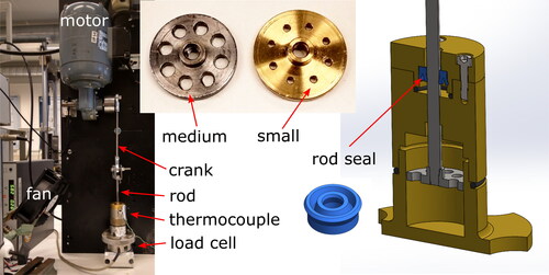
The rod has a very smooth finish, necessary to obtain a proper sealing. The seal is a standard polyurethane U-cup rod seal that provides good sealing at the expense of some friction losses, which should be compensated for. Two grease plates are used, both with eight holes. One has holes with a medium diameter of 3.7 mm and the other one has small holes with a diameter of 1.85 mm.

Energy dissipated by shearing inside the holes will cause the temperature of the grease to increase. This temperature rise is measured at the outside wall with a thermocouple and is minimized by cooling down the walls with a strong air flow generated by a fan. It is desirable to minimize the temperature rise and keep the grease worker at a constant lab temperature of approximately 21°C. When the grease micro structure breaks down upon shearing, this will cause a change (decrease) in viscosity, which is registered as a changed (reduced) force amplitude over time at the load cell. This cannot be distinguished from a change in viscosity caused by a change in temperature over time. Therefore, it is important to keep the temperature as constant as possible during the aging process.

Typical shear rates

The shear rates inside an elastohydrodynamic lubrication contact for rolling bearings are equal to (Dyson and Wilson (16)) [1] $$\dot{\gamma }=\frac{\Delta u}{h},$$[1] and for the inlet of the contact, [2] $$\dot{\gamma }=\frac{{\left(2u_2+u_1\right)}^2}{3\left(u_1+u_2\right)h}.$$[2]

The film thickness is in the order of magnitude of 1 μm and speeds u₁,u₂ are in the order of 10 m/s. The difference in speed is very small but could be 1 m/s. Hence, the shear rates are in the order of magnitude of $\dot{\gamma }\approx {10}^6-{10}^7$  s⁻¹ (1).

In the grease worker, only a small portion of the grease will be sheared at maximum velocity because of the reciprocating motion. An even smaller portion will reach high shear rates at the walls, as will be explained in the section Velocity and Shear Rate Profile. For the grease plate with medium-sized holes and for the ASTM grease workers, the wall shear rate is in the order of ${\dot{\gamma }}_{\mathit{wall}}\approx {10}^3$ s⁻¹. For the grease plate with small holes, the wall shear rate is increased to an order of magnitude of ${\dot{\gamma }}_{\mathit{wall}}\approx {10}^4$ s⁻¹. Because most of the shearing takes place at lower velocities and away from the walls, and assuming perfect mixing, any portion of grease will have experienced a much lower average shear rate. For comparison, in the Couette aging machines as used by Zhou et al. (5), the rotational speed is constant and the shear rates are in the order of $\dot{\gamma }$ = 200 s⁻¹.

Hence, the degradation of grease in laboratory equipment is mild compared to that in an elastohydrodynamic lubrication rolling bearing contact. However, much of the grease will not travel through a contact in a rolling bearing. Grease will significantly degrade during the churning phase after which most of it will be located in semi-stationary reservoirs located under the grease cage and/or on the bearing shoulders, bleeding oil (17). Mechanical aging will definitely continue after this but at a much lower rate. During the churning phase, the friction torque (and therefore energy loss) will be caused by drag. Here the shear will be on the order of magnitude of $\dot{\gamma }$ = 500 s⁻¹, depending on the dimensions and operating conditions of the bearing.

Methods

Estimation of energy density

In the work of Zhou et al. (12) and Rezasoltani and Khonsari (4) the total amount of specific mechanical work done by the grease worker, or total amount of energy density E_gw, was calculated as [3] $$E_{gw}=\frac{1}{V_{gw}}\sum _{k=1}^{N_h}{\overline{F}}_{gw}(k)L_{\mathit{piston}},$$[3] where ${\overline{F}}_{gw}(k)$ is the average force at half stroke k, N_h is the number of half strokes, L_piston is the stroke length, and V_gw is the grease worker internal volume (15.2 cm³).

As can be seen in Fig. 2, the force waveform can have any shape. To properly take this variation into account it is better to take the integral of the force acting over an incremental distance ds rather than taking the average, resulting in an energy density [4] $$E=\frac{1}{V_{gw}}{\int }_0^{S}F(s)ds,$$[4] where $S=N_h{L}_{\mathit{piston}}$ is the total distance traveled. In the grease worker test setup, the force F_l is measured using a load cell as a function of time. The velocity v of the piston is measured, or could be reconstructed, as a function of time as well. Then, there is a seal friction force F_s, estimated using Eq [11][11] $$F_s(v,t)=\left(a_0{e}^{a_{1}t}+a_2\right)\hspace{0.17em}\text{sin}\hspace{0.17em}\left(a_3\tanh \left(a_{4}v\right)\right),$$[11] , which should be subtracted from the force measured at the load cell to get the force required to push the grease through the holes of the grease plate $F_g=F_l-F_s.$ The instantaneous power density required to push the grease through the holes is then given by [5] $$P_g(t)=\frac{F_{g}v}{V_{gw}},$$[5]

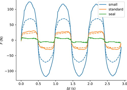
Figure 2. Force measured at the load cell for strokes 1–3 (solid line) and strokes 1,001–1,003 (dashed line). The waveform shape is sinusoidal-like for the grease plate with small holes and for the grease plate with medium-sized holes the shape is closer to a square wave, just like the force acting on the seal.

We can subsequently compute the total energy density up to a certain point in time T from the integral [6] $$E_g={\int }_0^T{P}_g(t)dt,$$[6]

The stroke frequency f is constant, having a value of 1 Hz as prescribed by the ASTM standard (13). Therefore, it is not strictly necessary to measure the velocity of the piston, but it can be reconstructed as well. The position s(t) of the piston is reciprocating in simple harmonic motion because the half stroke length is much smaller than the length of the connecting rod. With $v(t)=\frac{ds}{dt}$ we get the velocity signal as a function of time [7] $$v(t)=2\pi f\widehat{s}\hspace{0.17em}\text{sin}\hspace{0.17em}\left(2\pi ft\right),$$[7] where $\widehat{s}=\frac{1}{2}{L}_{\mathit{piston}}$ is the maximum amplitude for the piston and t is the time.

Stroke energy and power

The energy input can be calculated as a continuous integral as in Eq. [6][6] $$E_g={\int }_0^T{P}_g(t)dt,$$[6] , but because the energy input fluctuates during a stroke, and smooth plots are desired, we smooth the signal by calculating the energy density per stroke.

A stroke is a discrete event, which starts when the velocity is zero at time t_i and ends after a full stroke at time $t_{i+1}.$ The energy density E_s for stroke n_s having time interval t_i to $t_{i+1}$ is calculated from the integral [8] $$E_s(n_s)={\int }_{t_i}^{t_{i+1}}P(t\prime )dt\prime .$$[8]

The average power density P_s for stroke n_s can be defined in a similar way: [9] $$P_s(n_s)=\frac{1}{t_{i+1}-t_i}{\int }_{t_i}^{t_{i+1}}P(t\prime )dt\prime .$$[9]

Then, the total amount of energy up to stroke number N is the cumulative sum of each of the strokes [10] $$E_g=\sum _{k=1}^N{E}_s(k).$$[10]

Seal friction

The force F_l measured at the load cell needs to be corrected with seal friction F_s to obtain the force F_g required to push the grease through the holes of the grease plate. As will be shown in the section Seal Friction Results, the measured seal friction can be described by [11] $$F_s(v,t)=\left(a_0{e}^{a_{1}t}+a_2\right)\hspace{0.17em}\text{sin}\hspace{0.17em}\left(a_3\tanh \left(a_{4}v\right)\right),$$[11] where t is the time, v is the piston velocity, and a₀ to a₄ are the fitting parameters.

Estimation of viscosity

The viscosity of a lubricating grease is very dependent on the shear rate; the viscosity decreases with increasing shear rate. This is called shear thinning behavior, and the most commonly used model that describes this behavior with reasonable accuracy over a large range of shear rates is the Carreau model (18, 19). [12] $$\eta ={\eta }_{\infty }+\left({\eta }_0-{\eta }_{\infty }\right){\left(1+{\left(\lambda \dot{\gamma }\right)}^2\right)}^{\frac{m-1}{2}},$$[12] where η₀ is the viscosity at very low shear rates and ${\eta }_{\infty }$ the viscosity at infinitely high shear rates, approaching the base oil viscosity. The parameters λ and m are the Carreau model time constant and flow behavior index.

As described in the section Typical Shear Rates, the typical shear rates are in the range of 10² to 10⁴ ${\mathrm{s}}^{-1}.$ For a typical grease, this shear rate range is in the middle of the shear-thinning region, so the shear rate–dependent viscosity can be described well by the much simpler power law model (1) [13] $$\eta =K{\dot{\gamma }}^{n-1},$$[13] with K and n the flow consistency and flow behavior index, respectively.

The flow of grease through the holes of the grease plate can be considered as a pipe flow through a very short section of a circular pipe, for which a relatively simple expression for a power law fluid can be used (20): 14 $$\Delta P_p=\frac{2KL}{R}{\left(\frac{Q\left(3n+1\right)}{\pi R^{3}n}\right)}^n.$$14

Here the flow rate Q and pressure drop $\Delta P_p$ can be derived from the piston force F_g and piston velocity v, as will be shown in the section Fit to Power Law Model. The only unknown parameters are the flow consistency and shear thinning indexes K and n. These parameters can be solved for because within each stroke the piston velocity is varying sinusoidally, in a range of flow rates and pressure differences; see Fig. 7. The flow rates and pressure differences can be estimated using only the measured force, piston velocity, and dimensions of the grease worker.

First, the flow rate through a single hole can be calculated from the piston velocity, assuming that the flow rate is equal for all holes and that the grease is incompressible: [15] $$Q=\frac{1}{4}\frac{\pi d_p^{2}v}{n_h}.$$[15]

Secondly, the pressure drop over the grease plate is given by a [16] $$\Delta P_g=\frac{4F_g}{\pi d_{gw}^2}.$$[16]

The flow of grease from the reservoir to the inlet of the short pipes in the grease plate and from the outlet into the other reservoir present an additional entry and exit pressure loss that should be accounted for (20): [17] $$\Delta P_g=\Delta P_p\left[1+2\left(\frac{0.6D}{2L}\frac{3{(3n+1)}^2}{2(2n+1)(5n+3)}\right)\right],$$[17] where $\Delta P_p$ is the pressure loss in the pipe in the grease plate, which is corrected using a factor including the diameter D and length L of the pipe and the flow consistency index n. This gives the total pressure loss $\Delta P_g,$ which is derived from the force measured using the load cell at the bottom of the grease worker.

Finally, there is a gap between the wall of the grease worker and piston where some grease will flow as well. It was estimated using a power law model for slit flow that the contribution was negligible, so for simplicity of the model presented here this flow is not included.

Velocity and shear rate profile

The flow of a power law fluid through a circular pipe with radius R has a velocity profile given by (20) [18] $$u(r)=\frac{R}{1+\frac{1}{n}}\frac{Q\left(3n+1\right)}{\pi R^{3}n}\left[1-{\left(\frac{r}{R}\right)}^{1+\frac{1}{n}}\right].$$[18]

The shear rate is given by the derivative of the velocity profile $\dot{\gamma }=\frac{du}{dr},$ giving [19] $$\dot{\gamma }(r)=\frac{Q{\left(\frac{r}{R}\right)}^{1+\frac{1}{n}}\left(3n+1\right)}{\pi R^{2}nr}.$$[19]

The wall shear rate can be calculated by taking r = R, [20] $${\dot{\gamma }}_{\mathit{wall}}=\frac{Q\left(3n+1\right)}{\pi R^{3}n}.$$[20]

For parallel-plate rheometry, the viscosity is evaluated at a shear rate value located at the edge of the plate (20). Following similar reasoning for the circular pipe (20), one could take the wall shear rate. The problem, however, is that for the grease plate with small holes this shear rate is one order of magnitude larger than for the parallel-plate geometry of the rheometer, so comparing the evaluated viscosities becomes difficult. A solution is to evaluate the viscosity at a weighted average shear rate, given by [21] $$\overline{\dot{\gamma }}=\frac{1}{A}{\int }_A\dot{\gamma }dA\prime =\frac{1}{\pi R^2}{\int }_0^R\dot{\gamma }2\pi \mathit{rdr}=\frac{2Q(3n+1)}{\pi R^{3}n(2+\frac{1}{n})}.$$[21]

Computational fluid dynamics model

The complexity of the grease flow problem was reduced by assuming that it can be described using a simple pipe flow model. To validate this reduction of complexity, particularly the pressure loss correction of Eq. [17][17] $$\Delta P_g=\Delta P_p\left[1+2\left(\frac{0.6D}{2L}\frac{3{(3n+1)}^2}{2(2n+1)(5n+3)}\right)\right],$$[17] , a numerical model was made using COMSOL Multiphysics (21). COMSOL was earlier used to model grease flow, by Westerberg et al. (22), where the flow of grease inside the grease pockets of a double restriction seal geometry was studied. For stationary, incompressible, and laminar flow (creep flow), neglecting the inertial term (Stokes flow) and external forces, the Navier-Stokes equation reduces to (23) [22] $$0=-\nabla p+\nabla ·(\eta (\nabla \mathit{u}+{(\nabla \mathit{u})}^T)),$$[22] where p is the fluid pressure, u is the fluid velocity, and η is the shear rate–dependent viscosity (12) of the fluid. In COMSOL, this equation is solved together with the continuity equation [23] $$\rho \nabla ·\mathit{u}=0,$$[23] where ρ is the density of the fluid. The geometry of the fluid domain is modeled as shown in Fig. 3. Instead of using a moving piston in a static cup, the model is simplified to resemble a fluid flow through a pipe, where the grease plate acts as flow restriction. To save computational time, the whole grease plate with eight holes was not modeled, but by using symmetry the total model volume can be reduced to a pie piece of 1/16th of the original fluid volume. The dimensions can be found in Table 1 and the following boundary conditions were applied:

Figure 3. Front (a) and back (b) views of the fluid domain.

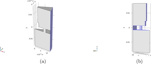
Table 1. Most relevant dimensions of the grease worker.

	Grease plate hole size
	Medium	Small
Cup inner diameter dgw (mm)	24
Cup inner height hgw (mm)	32.9
Maximum amplitude $\widehat{s}$ (mm)	13.8
Rod diameter drod (mm)	5.0
Piston thickness hpiston (mm)	2.9
Piston diameter dpiston (mm)	23.3	23.7
Hole diameter dhole (mm)	3.7	1.85

• The inlet grease velocity at the bottom is equal to the piston velocity.

• The outlet boundary condition at the top is set a pressure of 0 Pa.

• The two sides of the pie piece have a symmetry boundary condition.

• The walls of the piston, hole, and rod as indicated in Fig. 3(b) have a no-slip condition.

• The wall of the cup, as indicated in Fig. 3(a), has a no-slip condition with sliding a wall in the z-direction, equal to the grease velocity. This is necessary because in the grease worker, the piston moves relative to the cup and the bulk of the grease, both with zero velocity. In this model this is reversed: The piston has zero velocity and the grease moves relative to the piston, so the cup wall needs to have the same velocity as the grease.

For the mesh, a physics-controlled mesh with finer elements was selected, resulting in approximately 306,000 elements. A GMRES linear iterative solver was used to solve the equations, with a tolerance-based termination at a (default) value of 0.001.

Results

Seal friction results

The influence of seal friction is quite significant for the grease plate with the medium-sized holes. Depending on the type of grease and amount of degradation, this force can be as much as 50% of the measured peak force at the load cell. Any variation in this force leads to significant errors in the energy calculations and in the estimation of the parameters for the power law model. The seal friction force is measured regularly between grease aging experiments to obtain an average seal friction force signal and is done by running the grease worker for an hour without grease, while keeping the seal lubricated with grease.

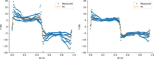
As can be seen in Fig. 4, there is quite some spread and the waveform shape is not a true square wave. The spread is smaller after 1,000 strokes. This figure also shows that the force increases at the edges of the square wave where the velocity of the piston approaches zero. This could be an indication of stick–slip effects. This is confirmed when the piston force is plotted against the piston velocity.

Figure 4. Seal friction force as a function of time, empty grease worker, eight measurements and the fit. The left graph shows the first stroke and the right graph shows stroke 1,000 for all of the eight measurements.

The solid line in Fig. 5 is a fit of the seal friction force using Eq. [11][11] $$F_s(v,t)=\left(a_0{e}^{a_{1}t}+a_2\right)\hspace{0.17em}\text{sin}\hspace{0.17em}\left(a_3\tanh \left(a_{4}v\right)\right),$$[11] . This equation was chosen such that there is a good fit at the higher, more important velocities. At these velocities, the spread in seal force is approximately ±2 N, but this spread becomes much larger at lower velocities of the piston. This is why, as we will see in the section Fit to Power Law Model, only the higher piston velocities will be used to estimate the parameters of the power law model fit. The fiting parameters for Eq. [11][11] $$F_s(v,t)=\left(a_0{e}^{a_{1}t}+a_2\right)\hspace{0.17em}\text{sin}\hspace{0.17em}\left(a_3\tanh \left(a_{4}v\right)\right),$$[11] are a₀ = 1.44 N, a₁ = 2.76 $\times {10}^{-3}{\mathrm{s}}^{-1},$ a₂ = 7.12 N, a₃ = 2.27 and a₄ = 4.78 $\times {10}^1\mathrm{s}{\mathrm{m}}^{-1}.$

Figure 5. Seal friction force as a function of velocity, empty grease worker, 8 measurements and the fit. The left graph shows the first stroke and the right graph shows stroke 1,000 for all of the eight measurements.

Power density master curve

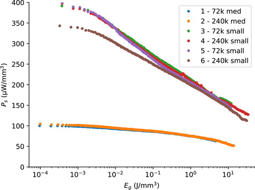
In the work of Zhou et al. (12), the yield stress was plotted against the cumulative energy density to obtain a master curve for the change in yield stress as a function of energy input. A similar method will be employed in the section Fit to Power Law Model, but instead of using the yield stress, the viscosity at the relevant shear rate will be plotted as a function of energy input. In this section we will show a slightly different master curve. Figure 6 shows the average stroke power density against the cumulative energy density for an Li/M grease. Under isothermal conditions, a change in stroke power density indicates a change in grease micro structure, which should be reflected by a change in rheological properties. Obtaining this graph using only the measured force signal F_l involves the following steps:

Figure 6. Stroke power density as a function of cumulative energy density for Li/SS grease.

• High-pass filtering of the force signal F_l with a cut off frequency of 0.5 Hz to remove the DC component of the signal, caused by the weight of sample, static friction of the seal, etc.

• Finding zero crossings in the force signal for reconstruction of the piston velocity signal.

• Reconstruction of the piston velocity signal v using Eq. [7][7] $$v(t)=2\pi f\widehat{s}\hspace{0.17em}\text{sin}\hspace{0.17em}\left(2\pi ft\right),$$[7] .

• Discarding the first two and last two strokes to exclude running-in and running-out effects.

• Calculating the instantaneous power density P_g using Eq. [5][5] $$P_g(t)=\frac{F_{g}v}{V_{gw}},$$[5] , which involves a correction for the friction losses at the seal.

• Calculating the stroke power density P_s using Eq. [9][9] $$P_s(n_s)=\frac{1}{t_{i+1}-t_i}{\int }_{t_i}^{t_{i+1}}P(t\prime )dt\prime .$$[9] .

• Calculating the cumulative energy density E_g using Eq. [6][6] $$E_g={\int }_0^T{P}_g(t)dt,$$[6] or [10].

In the plot of Fig. 6, two groups of lines can be distinguished. The lower group of lines, measurements 1 and 2, is for the plate with mediu-sized holes, with an initial stroke power density of 100 µW/mm³. The upper group of lines is for the grease plate with the small holes, reaching initial stroke power density levels of 400 µW/mm³. The number of strokes for aging is either 72,000 or 240,000 strokes. Note that the initial stroke energy of measurement 6 is 50 µW/mm³ below that of measurements 3 to 5. This is attributed to a higher initial temperature of 23°C instead of the normal temperature of 21°C.

Fit to power law model

To obtain the coefficients K and n of the power law model, the calculation is made using the following steps:

• Calculate the pressure difference $\Delta P_g$ and the flow rate Q using Eqs, [15]–[17].

• In the section on seal friction, the uncertainty in the correction when correcting for seal friction is ±2 N. This results in an uncertainty of pressure of 4.7 kPa.

• Fitting all of the strokes would take too much calculation time and is not useful because most of the change will occur in the first 100–1,000 strokes. Therefore, a selection of 50 strokes per decade with logarithmic spacing is taken to obtain approximately 250 points.

• For each of these strokes, a fit is made to the power law model of circular pipe flow of Eq. [14].

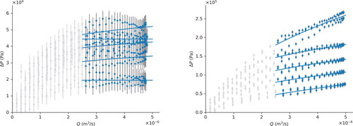
Figure 7 shows the pressure drop $\Delta P_g$ as a function of flow rate Q. It can be seen in Fig. 7(a) that the uncertainty in pressure difference of 4.7 kPa is quite significant for the grease plate with medium-sized holes. Figure 7(b) shows the results for the grease plate with small holes. The small holes configuration gives much smoother curves.

Figure 7. The pressure drop $\Delta P_g$ as a function of flow rate Q for a full stroke of measurements 2 and 4 for a grease plate with (left) medium-sized and (right) small holes. To illustrate the quality of the more clearly, only the first stroke, the last one, and three strokes in between are shown.

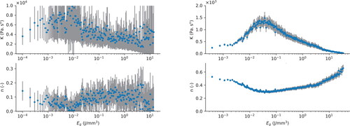
Figure 8 shows the resulting fitting coefficients for each of the approximately 250 selected strokes. The uncertainty in the pressure difference is clearly reflected in the error margins of the fitting coefficients, especially for the medium-sized holes version.

Figure 8. Resulting fitting coefficients as a function of energy density: (left) medium-sized holes and (right) small holes.

Validation with the rheometer

To validate the power law fitting coefficients as estimated using the method in the section Estimation of Viscosity, the viscosity calculated using this method can be compared with the flow curve measured using a rheometer. This was done for the same six samples of Li/M grease used in the section Power Density Master Curve. A sample of fresh grease was measured as well.

Because we want to obtain the flow curve at shear rates larger than 100 s⁻¹, the flow curve is not measured using a rotational sweep (24), but with an oscillatory sweep (25, 26). Using the Cox-Merz rule (1), the complex viscosity as a function of oscillation amplitude is converted to the real viscosity as a function of shear rate (i.e., the flow curve). A 25-mm smooth plate–plate geometry was used for all measurements. The measurements were done at a temperature between 21 and 23 °C in order to be as close as possible to the temperature of the grease in the grease worker. In order to achieve a high shear rate of 1,000 s⁻¹ with reasonable amplitude while keeping the grease in place, a very small gap size of 50 µm was chosen. It was checked that larger gap sizes had no influence on the results at higher shear rates.

The steps involved to obtain the flow curve were as follows:

• Use the filling and trimming procedure of Cyriac et al. (26).

• Wait until the temperature stabilizes at 22 C.

• Start with a gap size of 150 μm.

• Start with a preshear strain sweep; that is ramp up the strain from 0.01 to 3000% and ramp down back to 0.01, in steps of six points per decade, at an oscillation frequency of 10 rad/s.

• Repeat using the same settings for the actual measurement strain sweep.

• Reduce the gap to 50 μm, using the same sample, and trim off the excess grease.

• Repeat the preshear and measurement strain sweeps with a strain up to 10,000% to obtain a strain rate of 1,000 s⁻¹ at the gap size of 50 μm.

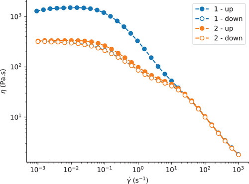
Figure 9 shows the flow curve of sample 4. The blue line shows the first up- and down-ramp, the preshear strain, and the orange line shows the second up- and down-ramp, the actual measurement. Only the first up-ramp is different from the others at low to medium shear rates. This could be caused by effects like fiber alignment. At the shear rates of interest—that is above 100 s⁻¹—all curves coincide. The curves for the 150-μm gap are not shown in Fig. 9, but they coincide nicely with the 50-μm gap for high shear rates.

Figure 9. Flow curve for sample 4, at a gap size of 50 μm.

Figure 10 shows the flow curve of the rheometer measurements for fresh Li/M grease, 72,000 and for 240,000 strokes. The red marks show the viscosity as calculated using the method described in the section Fit to Power Law Model for the same number of strokes. The fit as shown in Figs 7 and 8 was done and consequently is only valid for a small flow rate range. Using Eq. [21][21] $$\overline{\dot{\gamma }}=\frac{1}{A}{\int }_A\dot{\gamma }dA\prime =\frac{1}{\pi R^2}{\int }_0^R\dot{\gamma }2\pi \mathit{rdr}=\frac{2Q(3n+1)}{\pi R^{3}n(2+\frac{1}{n})}.$$[21] the average shear rate range is 287 to 547 s⁻¹ for the grease plate with medium-sized holes and 2,559 to 5,047 s⁻¹ for the grease plate with small holes.

Figure 10. Flow curve from rheometer measurements (denoted by “rheo”) and grease worker power law fit (denoted by “gw”) for the (a) medium-sized hole grease plate and (b) small hole grease plate.

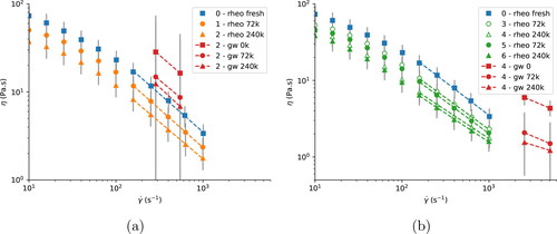
According to the DIN standards for grease measurement (24, 25), the reproducibility is 8 to 10% for an NLGI2 grease. When taking variation of instruments and operators in account, the error reaches a value of 27%. In other literature (27), an error of 24% was reported when comparing the plastic viscosity obtained using various types of rheometer geometries like parallel-plate, coaxial cylinder, and vane geometries. Because the grease worker could be considered as a different type of rheometer geometry, an error of 27% is acceptable and is taken as error on the rheometer measurements as shown by the error bars in Fig. 10.

For the grease plate with medium-sized holes, as shown in Fig. 10(a), sample 2 was taken to compare the grease worker and rheometer data. As could be expected from the error bars in power law fit, (see Fig. 7a), the error in viscosity is enormous and the value for the viscosity is a factor of 3 higher than the viscosity measured using the rheometer. The relative change in viscosity is also not consistent with the rheometer measurements.

Improvement can be seen for the grease plate with small holes; see Fig. 10(b). The error is much smaller, approximately 20% for the fresh grease and up to 65% for the degraded grease. The relative change is consistent with the rheometer measurements. Unfortunately, the absolute value of viscosity is overestimated again by a factor of 3. Additionally, it should be noted that the viscosity of samples 3 and 4 is slightly higher than that of samples 5 and 6. Samples 3 and 4 were measured 10 months after aging, so perhaps the grease microstructure was restored in this period of time, resulting in a higher viscosity.

Concluding, it is possible to measure the viscosity in situ in a grease worker with a small error for the small hole grease plate configuration. Unfortunately, compared to measurements with a plate–plate rheometer, the measured viscosity is a factor of 3 larger for both grease plates. This is ascribed to the difference in methodology, as will be explained in the ’Discussion’. A clear strength of the present methodology is that the grease worker can be used to monitor the relative changes in viscosity. This will be shown in the next section.

Viscosity (change) master curves

So far the adopted grease worker was used to measure the grease viscosity. In this section, the change in viscosity as a function of the imposed energy is addressed.

Figure 11 shows the change in viscosity as a function of energy input. The dots represent the relative change in viscosity as estimated from the fitting parameters of the section Fit to Power Law Model and the three lines are the change in viscosity measured using the rheometer.

Figure 11. Viscosity change as a function of cumulative energy.

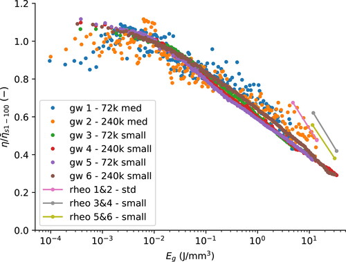
Using the medium-sized hole grease plate gives a large spread. The viscosity is therefore normalized using the mean viscosity of the first 100 strokes. The data points of the small hole grease plate start slightly above 1 and for the grease plate with medium-sized holes slightly above 0.8. The viscosity is evaluated at a weighted shear rate, as explained in Eq. [21][21] $$\overline{\dot{\gamma }}=\frac{1}{A}{\int }_A\dot{\gamma }dA\prime =\frac{1}{\pi R^2}{\int }_0^R\dot{\gamma }2\pi \mathit{rdr}=\frac{2Q(3n+1)}{\pi R^{3}n(2+\frac{1}{n})}.$$[21] , which is within the range of shear rates used for fitting the power law model. For the medium-sized holes grease plate and rheometer fit, the maximum shear rate has a value of 547 s⁻¹ and for the small hole grease plate this value is 5,047s⁻¹.

The normalized viscosity measurements measured using plates with different hole sizes collapse into a single curve by plotting this against energy rather than time. Note that the degradation rate after a certain time is larger for the small hole grease plate than for the large hole grease plate. When comparing the 240,000 strokes samples, the medium-sized holes grease plate (sample 2) has a reduction in viscosity of 62% at an energy input density of 13.9 J/mm³ whilst the grease plate with small holes (sample 6) has a reduction of 73% an an energy input density of 30.8 J/mm³. Comparing the measurements with those obtained from a plate–plate rheometer shows that the reduction is slightly less and that the slope is different. Because the data points of samples 1 and 2 and samples 5 and 6 are nicely aligned, it does confirm that the grease plate with small holes results in more degradation in the same amount of time.

The normalized viscosity measurements using the grease plate with the small holes is shown again separately in Fig. 12 to show clearly that it has much less scatter than the measurements done using the grease plate with medium sized holes. The fit is done using a grease aging equation, established in earlier work by Zhou et al. (12): [24] $$Y=\frac{Y_i-Y_{\infty }}{1+\kappa E_g^{\beta }}+Y_{\infty },$$[24] where Y represents the rheological property as a function of the imposed energy E_g. Because we are interested in the change in viscosity, we can write $Y=\eta /{\eta }_{s1},$ where ${\eta }_{s1}$ is the viscosity estimated in the first stroke. The parameter Y_i is the initial relative viscosity for fresh grease, $Y_i={\eta }_{s1}/{\eta }_{s1}=1.$ The final relative viscosity $Y_{\infty }$ is limited by the base oil viscosity having a value of η_b = 0.374 Pa s, so we can take $Y_{\infty }={\eta }_b/{\eta }_{s1}=0.0788.$ For the other two parameters are used as fitting parameters, the coefficient of degradation κ has a value of 0.911 (mm³/J) and the exponent of degradation β has a value of 0.418.

Figure 12. Viscosity change as a function of cumulative energy for the grease plate with small holes and the fit using Eq. [24][24] $$Y=\frac{Y_i-Y_{\infty }}{1+\kappa E_g^{\beta }}+Y_{\infty },$$[24] .

Computational fluid dynamics results

As explained in the section Computational Fluid Dynamics Model, the computational fluid dynamics (CFD) model uses the Carreau fluid to model the shear thinning behavior of the grease. The simulations are done with both grease plates using the same parameters for the Carreau model. These parameters have values of η₀ = 1462 Pa s, ${\eta }_{\infty }$ = 0.374 Pa s, λ = 8.32 s, and m = 0.413. The motivation will be explained in detail in the Discussion.

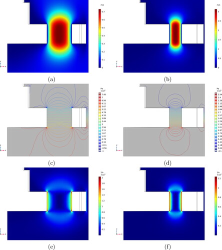
The 2D plots for the velocity, pressure, and shear rate are shown in Fig. 13. The isobars (lines with constant pressure) for the grease plate with small holes, (Fig. 13d), show a fully developed flow at the full length of the pipe, whereas entrance effects are are clearly visible in the grease plate with medium-sized holes. The CFD model can also be used to look into the details of the flow through the gap between the piston and wall. For the grease plate with small holes this is 1.9% of the total flow. Although the pressure difference for the grease plate with medium-sized holes is almost four times smaller, the gap is larger and the flow through this gap is 4.5% of the total flow, becoming a significant contribution.

Figure 13. (a), (b) Velocity, (c), (d) pressure, and (e), (f) shear rate at the maximum plate velocity for the grease worker where the grease plates are executed with medium-sized and small holes.

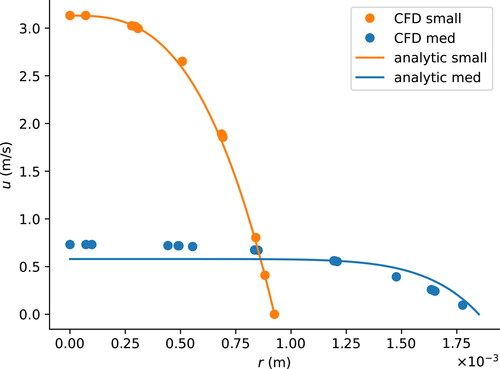
A comparison between the velocity profile of the CFD model and the analytic model (Eq. [18][18] $$u(r)=\frac{R}{1+\frac{1}{n}}\frac{Q\left(3n+1\right)}{\pi R^{3}n}\left[1-{\left(\frac{r}{R}\right)}^{1+\frac{1}{n}}\right].$$[18] ) is shown in Fig. 14. The parameters K and n for the analytic power law model were earlier shown in Fig. 7. There is a very good agreement for the grease plate with small holes, indicating that the power law model is a suitable description of the rheology in this shear rate domain. For the plate with medium-sized holes, the agreement is not a good due to the large difference in the slope parameter m = 0.409 of the Carreau model and n = 0.143 of the power law fit.

Figure 14. Comparison between the velocity profiles obtained from the CFD and analytic models.

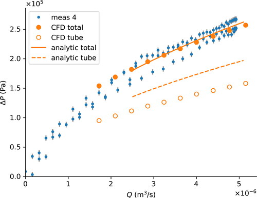
The pressure drop as a function of flow rate is plotted in Fig. 15, comparing the first stroke of measurement 4 with the CFD simulation and the analytic power law model. Equation [17][17] $$\Delta P_g=\Delta P_p\left[1+2\left(\frac{0.6D}{2L}\frac{3{(3n+1)}^2}{2(2n+1)(5n+3)}\right)\right],$$[17] is the total pressure drop, including a correction for the pressure loss caused by the flow from the reservoir into the short pipes, which is illustrated nicely in the 2D pressure plots of Fig. 13c and 13(d). The pressure drop over the tube as calculated by the CFD model and the analytic model using Eq. [14] can be compared using Fig. 15 as well. It can be seen that both models agree quite well with the measurements regarding the total pressure drop but that the pressure drop in the tube is overestimated in the analytic model compared to that in the CFD model.

Figure 15. Pressure drop as a function of flow rate. The comparison of the total pressure drop, including entrance and exit pressure losses, between measurement (blue dots), analytic model (solid orange line), and CFD model (orange closed dots). The comparison of the pressure drop in the tube only, analytic model (dashed orange line) and CFD model (orange open dots).

Discussion

As mentioned in the section Validation with the Rheometer, there is a factor of 3 difference between the viscosity of an Li/M grease measured using the rheometer and the grease worker. In this section we will discuss the rationale behind this.

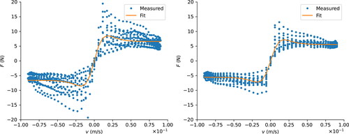
Figure 16 shows the flow curves. The blue dots represent the flow curve measured in oscillation mode, as in the section Validation with the Rheometer. The red line is the viscosity of the base oil, which does not depend on the shear rate. This also implies that the viscosity of the grease cannot be smaller than that. The blue line represents the best fit to the oscillatory measurements using the Carreau model (12). The green dots represent the flow curve measured in rotation mode, using a gap of 50 μm. It is well known that the viscosity at very low shear rates cannot be measured in a plate–plate rheometer with continuous rotation due to wall slip (1). At somewhat higher shear rates the results with continuous rotation and oscillatory shear are, as expected, equal. At the highest shear rates, the viscosity measured with continuous rotation is lower than that of the base oil, which is physically not possible. This could be attributed to slip effects, loss of grease, shear banding, heating effects, or a combination of these. The viscosities obtained from the grease worker for the two plates types are plotted in green and purple, similar to Fig. 10. The orange line, fit CFD, represents a Carreau flow curve, similar to the blue one, having identical parameters except for parameter m. In COMSOL an optimization is done for the m parameter, resulting in coinciding measured and calculated pressure drop as shown in Fig. 15 for the highest flow rate. Finally, there is the green-edged circle, rheo preshear, showing the viscosity after applying 1 second of preshear according to the DIN 51810-2 procedure.

Figure 16. Flow curve with various types of measurements and fits. Blue dots: rheometer in oscillating mode. Green closed dots: rheometer in continuous rotation mode. Green open dot: first second of preshear phase. Green dots connected by a line: grease worker with medium-sized holes. Purple dots connected by line: grease worker with small holes. Blue line: Carreau model with parameters obtained by fitting with the rheometer in oscillating mode. Orange line: Carreau model using the m parameter obtained from the CFD calculations.

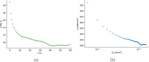
The DIN standard (24) for a rheometer with a cone–plate geometry prescribes a 60-s preshear phase at a shear rate of 100 s⁻¹ prior to performing the measurement in rotational mode. Figure 17(a) shows the evolution of the viscosity during this period, measured with the plate–plate geometry and gap size 50 μm. The viscosity drops from 21 Pa.s to approximately 10 Pa.s; that is, a factor of 2! During this preshear ${10}^{-2}$ J/mm³ was used, which is quite significant. In the grease worker the same amount of energy gives a viscosity reduction of less than only 10%, as can be seen in Fig. 11. An explanation for this could be that preshearing in the rheometer is continuous in one direction, which causes the fibers of the Li/M grease to align (before possibly breaking up/degrading due to shear aging). This alignment already causes a large reduction in viscosity. This could be thixotropic, if the change is time-dependent and reversible (28). In the grease worker this effect should not play a role. Only a very small portion of the grease is sheared at the walls of the holes in the grease plate, at a much larger shear rate (up to 10⁴ s⁻¹) for a very short amount of time (approximately 1 ms). This portion of heavily sheared and slightly degraded grease is subsequently mixed with the bulk of grease. So, on average, the viscosity decreases only slightly and alignment only happens for a short amount of time within the holes of the grease plate but will not persist after mixing with the bulk of the grease. This effect applies not only to fresh grease but also to grease that is degraded using the grease worker, as shown in Fig. 10 and explained in the section Validation with the Rheometer.

Figure 17. Preshear with a constant shear rate of 100 s⁻¹ following DIN 51810-2: (a) viscosity as a function of time and (b) power density as a function of energy density.

Conclusions

The grease worker is a standard instrument to qualify the shear stability of lubricating greases. The results of the difference in grease consistency before and after working a grease can be found in the specifications for all lubricating greases for rolling bearings. The method has not essentially changed since 1956. However, in the last decades it was recognized that the instrument can also be used to study shear degradation more fundamentally.

This started with earlier work (4–6) where the grease worker was used to mechanically degrade lubrication grease and to calculate the energy and/or generated entropy required to do that using the force measured with a load cell located at the bottom of the cup. In this article, a refined method is presented to calculate/measure the response of the rheological properties of grease to this energy input. A great advantage is that this change in rheological properties can be monitored in eliminating the need to do separate measurements using a rheometer to obtain these properties but also giving the advantage that it is no longer necessary to use new grease samples for each measurement, leading to an increase in reliability. A power law fluid pipe flow model is applied for that purpose. Its validity is verified using CFD simulations and measurements using a rheometer with a plate–plate geometry.

To improve the accuracy and decrease the time needed to degrade the grease, a new grease plate was made with holes half the size of the original ones. The time to obtain the same amount of degradation was thereby reduced by almost a factor of 4. This also led to an increase in accuracy because the required force to push the grease through the holes was now much larger compared to the seal friction force. After subtracting the friction force from the force measured at the load cell, the remaining variations in this friction force were estimated at 2%. This led to an error in viscosity of about 20% for fresh Li/M grease and up to 65% for degraded Li/M grease. This is very good because the standard equipment has error margins between 8% and 27% (27). Further improvements can be made if the seal friction can be reduced without compromising its sealing performance and by measuring the seal friction immediately before and after each measurement.

There is a difference of a factor of 3 between the viscosity value as estimated using the grease worker and a standard rheometer measurement. This does not mean that the viscosity measured using the grease worker is wrong. There are also flaws in the methodology followed using the standard plate–plate rheometer, which are often not recognized when the viscosity of a complex material such as lubricating grease is measured. One of these can be attributed to the measurement principle of a plate–plate rheometer itself. In plate–plate rheometry, continuous shear in one direction probably aligns the fibers, causing a large decrease in measured viscosity in 30 s, as shown in Fig. 17. This alignment also happens in the holes of the grease plate but only for a very short amount of time, in the order of 1 ms. This portion of heavily sheared and slightly degraded grease is then mixed with the bulk of grease, so that the next stroke starts with nonaligned grease fibers, creating a different situation as with the plate–plate rheometer. This mixing also takes place in a rolling bearing, making the grease worker more relevant compared to a standard plate–plate rheometer. Despite the fact that there is a difference in absolute viscosity, it is shown in this article that the relative change as measured with the grease worker is close to the change measured using the rheometer. This makes this technology very useful in measuring the rheology of lubricating greases, particularly for studying the change during mechanical degradation.

Improvements could be made by tuning any of the dimensions to the grease being studied. For instance, a change in size and/or amount of holes in the grease plate could improve the accuracy of the viscosity measurement and/or increase the speed of degradation. The reciprocating frequency could be made variable in order to study a larger range of shear rates and one could study the effect of making noncircular holes; for example, slits.

Nomenclature
A	=	Area (m2)
f	=	Stroke frequency (Hz)
dp	=	Piston diameter (m)
dgw	=	Inner diameter of the grease worker (m)
D	=	Hole diameter (m)
E	=	Total input energy density of the grease worker (J/mm3)
Eg	=	Total input energy density of the grease (J/mm3)
Egw	=	Total input energy density of the grease worker (4, 12) (J/mm3)
Eseal	=	Energy density dissipated at seal at stroke ns (J/mm3)
Es	=	Energy density of the grease at stroke ns (J/mm3)
F	=	Force (N)
Fl	=	Force measured using the load cell (N)
Fg	=	Force exerted on the grease (N)
${\overline{F}}_{gw}$	=	Average force as defined in the literature (4, 12) (N)
Fs	=	Friction force at the seal (N)
K	=	Power law model flow consistency index (Pa sn)
L	=	Length of the pipe (m)
Lpiston	=	Length of a stroke (m)
m	=	Carreau model flow behavior index
n	=	Power law model flow behavior index
ns	=	Stroke number
nh	=	Number of holes
Nh	=	Number of half strokes
p	=	Fluid pressure (Pa)
P	=	Power density (W/mm3)
Ps	=	Average power density for stroke Ns (W/mm3)
Q	=	Grease flow rate through a single hole (m3/s)
r	=	Radius (m)
R	=	Hole radius (m)
t	=	Time (s)
u	=	Grease velocity (m/s)
v	=	Piston velocity (m/s)
Vgw	=	Internal volume of the grease worker (mm3)
$\dot{\gamma }$	=	Shear rate (s−1)
$\overline{\dot{\gamma }}$	=	Average shear rate (s−1)
${\dot{\gamma }}_{\mathit{wall}}$	=	Wall shear rate (s−1)
$\Delta P_g$	=	Pressure difference between sides of the grease plate (Pa)
$\Delta P_p$	=	Pressure difference between ends of the pipe (Pa)
η	=	Viscosity (Pa s)
η0	=	Viscosity at low shear rates (Pa s)
ηb	=	Base oil viscosity (Pa s)
${\eta }_{s1}$	=	Viscosity of the first stroke (Pa s)
${\overline{\eta }}_{s1-100}$	=	Average viscosity of the first 100 strokes (Pa s)
${\eta }_{\infty }$	=	Viscosity at high shear rates (Pa s)
λ	=	Carreau model time constant (s)
ρ	=	Density (kg/m3)
ω	=	Angular velocity (rad/s)

Acknowledgements

We thank Leo Tiemersma for making the grease plate with small holes and other parts for the grease worker, Dr. Dirk van den Ende for discussions on rheology and the CFD model, Qierui Zhang for various discussions and help with the rheometer, and SKF for permission to publish this article.

References

- Lugt, P. (2013), Grease Lubrication in Rolling Bearings, 1st Ed., John Wiley & Sons: Chichester, UK.
- Ito, H., Tomaru, M., and Suzuki, T. (1988), “Physical and Chemical Aspects of Grease Deterioration in Sealed Ball Bearings,” Lubrication Engineering, 44(10), pp 872–879.
- Kuhn, E. (1998), “Investigations into the Degradation of the Structure of Lubricating Greases,” Tribology Transactions, 41(2), pp 247–250. doi:10.1080/10402009808983745
- Rezasoltani, A. and Khonsari, M. M. (2014), “On the Correlation Between Mechanical Degradation of Lubricating Grease and Entropy,” Tribology Letters, 56(2), pp 197–204. doi:10.1007/s11249-014-0399-8
- Zhou, Y., Bosman, R., and Lugt, P. M. (2018), “A Model for Shear Degradation of Lithium Soap Grease at Ambient Temperature,” Tribology Transactions, 61(1), pp 61–70. doi:10.1080/10402004.2016.1272730
- Osara, J. and Bryant, M. (2019), “Thermodynamics of Grease Degradation,” Tribology International, 137, pp 433–445. doi:10.1016/j.triboint.2019.05.020
- Acar, N., Franco, J. M., and Kuhn, E. (2020), “On the Shear-Induced Structural Degradation of Lubricating Greases and Associated Activation Energy: An Experimental Rheological Study,” Tribology International, 144, pp 106105. doi:10.1016/j.triboint.2019.106105
- Magnin, A. and Piau, J. M. (1987), “Shear Rheometry of Fluids with a Yield Stress,” Journal of Non-Newtonian Fluid Mechanics, 23, pp 91–106. doi:10.1016/0377-0257(87)80012-5
- Baart, P., Lugt, P. M., and Prakash, B. (2014), “On the Normal Stress Effect in Grease-Lubricated Bearing Seals,” Tribology Transactions, 57(5), pp 939–943. doi:10.1080/10402004.2014.935120
- Barnes, H., Hutton, J., and Walters, K. (1989), An Introduction to Rheology, Elsevier Science, AE Amsterdam.
- Hutton, J. F. (1975), “On Using the Weissenberg Rheogoniometer to Measure Normal Stresses in Lubricating Greases as Examples of Materials Which Have a Yield Stress,” Rheologica Acta, 14(11), pp 979–992. doi:10.1007/BF01516301
- Zhou, Y., Bosman, R., and Lugt, P. M. (2019), “A Master Curve for the Shear Degradation of Lubricating Greases with a Fibrous Structure,” Tribology Transactions, 62(1), pp 78–87. doi:10.1080/10402004.2018.1496304
- ASTM D1403-10. (2007), “Test Methods for Cone Penetration of Lubricating Grease Using One-Quarter and One-Half Scale Cone Equipment,” ASTM International: West Conshohocken, PA.
- American Society for Testing and Materials. (2008), “ASTM D217 Standard Test Methods for Cone Penetration of Lubricating Grease,” ASTM International: West Conshohocken, PA.
- Spiegel, K., Fricke, J., and Meis, K.-R. (2000), “The flow behavior of lubricating greases,” Vol. 500 of Kontakt & Studium, Schmierfette, W. Bartz (Ed.), pp 228–265, Expert Verlag, Renningen-Malmsheim.
- Dyson, A. and Wilson, A. R. (1965), “Paper 3: Film Thicknesses in Elastohydrodynamic Lubrication by Silicone Fluids,” Proceedings of the Institution of Mechanical Engineers, Conference Proceedings, 180(11), pp 97–112. doi:10.1243/PIME_CONF_1965_180_323_02
- Lugt, P. (2009), “A Review on Grease Lubrication in Rolling Bearings,” Tribology Transactions, 52(4), pp 470–480. doi:10.1080/10402000802687940
- Agassant, J.-F., Avenas, P., Carreau, P. J., Vergnes, B., and Vincent, M. (2017), Polymer Processing: Principles and Modeling, 2nd Ed., Carl Hanser: München, Germany.
- Carreau, P. J. (1972), “Rheological Equations from Molecular Network Theories,” Transactions of the Society of Rheology, 16(1), pp 99–127.
- Barnes, H. (2000), A Handbook of Elementary Rheology, University of Wales Institute of Non-Newtonian Fluid Mechanics, Penglais, United Kingdom.
- (2019), Comsol Multiphysics® Version 5.5. Comsol AB, Stockholm, Sweden.
- Westerberg, L. G., Sarkar, C., Farre Llados, J., Lundstrom, T. S., and Hoglund, E. (2017), “Lubricating Grease Flow in a Double Restriction Seal Geometry: A Computational Fluid Dynamics Approach,” Tribology Letters, 65(3).
- (2017), Comsol Multiphysics Cyclopedia. Available at: https://www.comsol.ch/multiphysics/navier-stokesequations. (accessed March, 2021).
- DIN 51810-1. (2011), Testing of lubricants - Determination of the shear viscosity of lubricating greases using the rotational viscometer - Part 1: Cone and plate measuring system. Berlin.
- DIN 51810-2. (2011), Testing of lubricants - Testing rheological properties of lubricating greases - Part 2: Determination of flow point using an oscillatory rheometer with a parallel-plate measuring system. Berlin.
- Cyriac, F., Lugt, P. M., and Bosman, R. (2015), “On a New Method to Determine the Yield Stress in Lubricating Grease,” Tribology Transactions, 58(6), pp 1021–1030. doi:10.1080/10402004.2015.1035414
- Haist, M., Link, J., Nicia, D., et al. (2020), “Interlaboratory Study on Rheological Properties of Cement Pastes and Reference Substances: Comparability of Measurements Performed with Different Rheometers and Measurement Geometries,” Materials and Structures, 53(4).
- Mewis, J. and Wagner, N. J. (2009), “Thixotropy,” Advances in Colloid and Interface Science, 147–148, pp 214–227. doi:10.1016/j.cis.2008.09.005