Modeling of Lewis number dependence of scalar dissipation rate transport for Large Eddy Simulations of turbulent premixed combustion

ABSTRACT

The influences of differential diffusion of heat and mass on the Favre-filtered scalar dissipation rate (SDR) transport have been analyzed and modeled using a priori analysis of Direct Numerical Simulations (DNS) data of freely propagating statistically planar turbulent premixed flames with different values of global Lewis number, Le. The DNS data has been explicitly filtered using a Gaussian filter to obtain the unclosed terms of the Favre-filtered SDR transport equation, arising from turbulent transport (T₁), density variation due to heat release (T₂), strain rate contribution due to the alignment of scalar and velocity gradients (T₃), correlation between the gradients of reaction rate and reaction progress variable (T₄), molecular dissipation of SDR (−D₂), and diffusivity gradients f(D). The statistical behaviors of these terms and their scaling estimates reported in a recent analysis have been utilized here to propose models for these unclosed terms in the context of Large Eddy Simulations (LES) and the performances of these models have been assessed using the values obtained from explicitly filtered DNS data. These newly proposed models are found to satisfactorily predict both the qualitative and quantitative behaviors of these unclosed terms for a range of filter widths Δ for all Le cases considered here.

Nomenclature

c	=	reaction progress variable
cm	=	thermo-chemical parameter
CP	=	specific heat at constant pressure
CV	=	specific heat at constant volume
CF	=	model parameter
C3, C4	=	model parameters
D	=	progress variable diffusivity
Dt	=	eddy diffusivity
Da	=	Damköhler number
D1	=	molecular diffusion term
D2	=	molecular dissipation term
fb	=	burning mode probability density function
	=	model parameters
f(D)	=	term due to diffusivity gradient
ksgs	=	sub-grid scale kinetic energy
	=	thermo-chemical parameter
Ka	=	Karlovitz number
Le	=	Lewis number
l	=	integral length scale
Ma	=	Mach number
Mi	=	ith component of resolved flame normal
Nc	=	scalar dissipation rate
Ni	=	ith component of flame normal
p	=	model parameter
Pr	=	Prandtl number
Q	=	general quantity
Ret	=	turbulent Reynolds number
ReΔ	=	sub-grid Reynolds number
	=	unstrained laminar burning velocity
t	=	time
tc	=	chemical time scale
tf	=	initial turbulent eddy turnover time
tsim	=	simulation time
T	=	instantaneous dimensional temperature
T+	=	non-dimensional temperature
Tad	=	adiabatic flame temperature
T0	=	reactant temperature
T1, T2, T3, T4	=	terms in the transport equation of Favre-filtered scalar dissipation rate
ui	=	ith component of nondimensional fluid velocity
u′	=	root mean square fluctuation of velocity
u′Δ	=	sub-grid velocity fluctuation
	=	chemical reaction rate
xi	=	ith Cartesian coordinate
YR	=	reactant mass fraction
YR0	=	reactant mass fraction in unburned gas
YR∝	=	reactant mass fraction in burned gas
αT	=	thermal diffusivity
αT0	=	thermal diffusivity of the unburned gas
β	=	Zel’dovich number
β3, β′3	=	model parameters
γ	=	ratio of specific heats (=CP/CV)
γ1, γ2	=	model parameter
δth	=	thermal flame thickness
δz	=	Zel'dovich flame thickness
Δ	=	filter width
Γ	=	model parameter
μ	=	viscosity
μ0	=	viscosity of unburned gas
ρ	=	density
ρ0	=	unburned gas density
τ	=	heat release parameter
τij	=	viscous stress tensor
Φ′	=	model parameter
	=	LES-filtered value of a general quantity q
	=	Favre-filtered value of a general quantity q
Subscripts	=
0	=	unburned gas value
∞	=	burned gas value
res	=	resolved scale value
sg	=	sub-grid scale value
Acronyms	=
DNS	=	direct numerical simulation
LES	=	large eddy simulation
pdf	=	probability density function
SDR	=	scalar dissipation rate

1. Introduction

Lean premixed combustion has been identified as one of the possible ways to reduce pollutant emission from gasoline engines and industrial gas turbines [1]. Lean hydrogen and hydrogen-blended hydrocarbon combustion has the potential to attenuate pollutants and greenhouse gas emissions [2, 3]. However, the flames with abundance of fast diffusing species such as hydrogen either in molecular or in atomic form give rise to a significant level of differential diffusion of heat and mass. The differential diffusion of heat and mass can be characterized by a nondimensional number known as the Lewis number Le, which is defined as the ratio of thermal diffusivity α_T to mass diffusivity D (i.e., Le = α_T/D). In actual premixed combustion it is often not straightforward to assign a single global Lewis number in the presence of several species with different Lewis numbers. Often the Lewis number of the deficient species is considered to be the global Lewis number [4], whereas Law and Kwon [5] proposed a methodology of evaluating the effective Lewis number based on heat release measurements. More recently Dinkelacker et al. [6] proposed an algebraic expression for the effective Lewis number based on mole fractions of major species. A number of previous analyses concentrated on the effects of global Lewis number on different aspects of premixed combustion in isolation [7–28] and the same approach has been adopted here.

Modeling of the differential diffusion arising from non-unity global Lewis number remains pivotal to high-fidelity engineering simulations, which are likely to play important roles in the development of new-generation combustors using either hydrogen or hydrogen-blended fuels. Prediction of the micro-mixing rate of hot products and cold unburned gas plays a key role in the modeling of turbulent reacting flows and a quantity known as the scalar dissipation rate (SDR) characterizes this micro-mixing rate [29, 30–32]. Furthermore, the Favre-mean value of SDR of reaction progress variable c in premixed turbulent flames can be related to the mean reaction rate in the context of Reynolds Averaged Navier Stokes (RANS) simulations [23, 33–35]. The instantaneous SDR of reaction progress variable is defined as [23, 33–38]

(1)

where D is the diffusivity of reaction progress variable c. Recent analyses have demonstrated [36–38] that the SDR-based reaction rate closure for RANS can also be used for the modeling of the filtered reaction rate based on the Favre-filtered SDR of a reaction progress variable (i.e., ) in the context of Large Eddy Simulation (LES) in the following manner when the filter size Δ remains greater than the thermal flame thickness δ_th = (T_ad − T₀)/Max| ∇ T|_L (where T_ad, T₀, and T are the adiabatic flame, unburned gas, and instantaneous temperatures, respectively):

(2)

where ρ is the density and is the Favre-filtered value of a quantity Q with the over-bar indicating an LES filtering operation. In Eq. (2) f_b(c) is the reacting mode probability density function (pdf) of c and the subscript “L” refers to the planar laminar flame conditions. By assuming f_b(c) as a smooth function, regardless of the exact form, the numerical value of c_mremains within a range of 0.7–0.9 for typical hydrocarbon–air mixtures [33].

The modeling of SDR not only is useful for the closure of filtered reaction rate but also plays a pivotal role in the closure of micro-mixing rate in the context of pdf methodology [30, 39–41]. For turbulent premixed flames, the Favre-filtered SDR can be modeled either by using an algebraic expression in terms of the resolved quantities or by solving a modeled transport equation. A few recent analyses [36–41] have concentrated on the algebraic closure of SDR for turbulent premixed flames in the context of LES. Algebraic closures are suitable when an equilibrium is maintained between the generation and destruction rates of , but this assumption may be rendered invalid under some conditions (e.g., low Damköhler number lean premixed combustion). A number of previous analyses [34, 42–51] concentrated on the modeling of SDR transport in turbulent premixed combustion in the context of RANS simulations. Interested readers are referred to Ref [34]. for a detailed review of the existing modeling methodologies for SDR transport in the context of RANS simulations. Recent advancements in high-performance computing have made LES of industrial flows more affordable than in the past, and LES is more successful in capturing unsteady flow features than RANS. However, relatively limited attention has been given to the investigation of SDR transport in the context of LES [52, 53]. Recently, models for the unclosed terms of the SDR transport equation for unity Lewis number flames in the context of LES have been proposed [53], but the differential diffusion effects due to non-unity Le were not addressed. A recent analysis [28] concentrated on the influences of global Le on the statistical behaviors of the unclosed terms of the transport equation based on an order-of-magnitude approach, which successfully explained the effects of global Le and the filter width Δ dependences of the Favre-filtered SDR and its transport. It has been found that Le has significant influences on both the qualitative and quantitative behaviors of the unclosed terms of the SDR transport equation [22, 28]; however, the modeling of Le effects on these unclosed terms is yet to be addressed, and the present analysis aims to address this gap in the existing literature. In this respect the main objectives of this paper are:

1. To propose models for the unclosed terms of the SDR transport equation in such a manner that the performances of these models remain satisfactory for a range of Δ and Le.

2. To assess the performances of the newly proposed models with respect to explicitly filtered Direct Numerical Simulation (DNS) data.

These objectives are addressed here by conducting a priori analysis using a DNS database of statistically planar turbulent premixed flames with a range of different values of Le (i.e., Le = 0.34–1.2). The details related to mathematical background and numerical implementation are provided in the next section. This is followed by the presentation of the results and subsequent discussion. The main findings are summarized and conclusions are drawn in the final section of this paper.

2. Mathematical background & numerical implementation

Three-dimensional DNS simulations with detailed chemistry are now possible, but they remain extremely expensive and need several millions of CPU hours [54] for conducting extensive parametric variations and carrying out explicit filtering of DNS data using a range of filter widths Δ, as has been carried out in the current study. Thus, the chemical mechanism has been simplified here as a single-step Arrhenius-type irreversible chemical reaction. Under this condition the species field is uniquely represented by a reaction progress variable c, which can be defined by using the mass fraction of a suitable reactant Y_R as c = (Y_R0 − Y_R)/(Y_R0 − Y_R∞), where subscripts 0 and ∞ denote the values in the unburned and burned gases, respectively. The transport equation of c can be used to derive a transport equation of , which takes the following form [28, 53]:

(3)

where u_i is the ith component of the velocity vector. On the left-hand side of Eq. (3) the terms denote the transient effects and resolved advection of , respectively. The term D₁ depicts the molecular diffusion of , and the terms T₁, T₂, T₃, T₄, (−D₂), and f(D) are all unclosed and expressed as follows:

(4i)

(4ii)

(4iii)

(4iv)

(4v)

(4vi)

where is the reaction rate of c. The term T₁ represents the effects of sub-grid convection, whereas T₂ denotes the effects of density-variation due to heat release. The term T₃ is determined by the alignment of ∇c with local strain rate e_ij = 0.5(∂u_i/∂x_j + ∂u_i/∂x_i), and this term is commonly referred to as the scalar-turbulence interaction term. The term T₄ arises due to the correlation between and ∇c, whereas (−D₂) denotes the molecular dissipation of SDR; these terms will henceforth be referred to as the reaction rate term and the dissipation term, respectively. The term f(D) denotes the effects of D variation. A priori DNS modeling of the above-mentioned unclosed terms will be discussed in Section 3 of this paper.

For the present analysis, a DNS database of freely propagating turbulent premixed flames has been considered. The simulation domain is taken to be a cube of 24.1δ_th × 24.1δ_th × 24.1δ_th, which is discretized using a uniform Cartesian grid of 230 × 230 × 230 points, ensuring about 10 grid points are kept within Min(δ_L, δ_th), where δ_L = 1/(Max |∇c|_L) is an alternative flame thickness based on |∇c| and the values of δ_L/δ_th for cases A–E (with Le = 0.34, 0.6, 0.8, 1.0, and 1.2) are provided in Table 1. The initial values of the normalized root-mean-square (rms) value of turbulent velocity u′/S_L, integral length scale to thermal flame thickness ratio l/δ_th, Damköhler number Da = lS_L/u′δ_th, Karlovitz number Ka = (u′/S_L)^3/2(l/δ_th)^−1/2, turbulent Reynolds number Re_t = ρ₀u′l/μ₀, and τ = (T_ad − T₀)/T₀ are presented in Table 1 along with domain and grid sizes, where ρ₀ and μ₀ are the unburned gas density and viscosity, respectively, and S_L is the unstrained laminar burning velocity. The flamelet assumption is likely to be valid for the values of u′/S_L and l/δ_th considered here, and all cases considered here represent the thin reaction zones regime combustion according to the regime diagram by Peters [55].

Table 1. Initial values of simulation parameters and nondimensional numbers relevant to the DNS database considered for this analysis.

Case	Le	u′/SL	δL/δth	l/δth	τ	Ret	Da	Ka
A	0.34	7.5	2.17	2.45	4.5	47.0	0.33	13.0
B	0.6	7.5	1.40	2.45	4.5	47.0	0.33	13.0
C	0.8	7.5	1.15	2.45	4.5	47.0	0.33	13.0
D	1.0	7.5	1.0	2.45	4.5	47.0	0.33	13.0
E	1.2	7.5	0.90	2.45	4.5	47.0	0.33	13.0

For all cases τ = 4.5; β = 6.0; Pr = 0.7;  = 0.014159.

The simulations have been carried out using a well-known DNS code called SENGA [56]. For all cases the boundary conditions in the mean flame propagation direction are considered to be partially nonreflecting, whereas boundaries in the transverse directions are considered to be periodic. A 10th order central difference scheme is used for spatial differentiation for the internal grid points and the order of differentiation gradually drops to a one-sided second-order scheme at the non-periodic boundaries. A low-storage third-order Runge-Kutta method is used for explicit time advancement for all the governing equations. In all cases flame–turbulence interaction takes place under decaying turbulence, which necessitates the simulation time t_sim ≥ max(t_f, t_c), where t_f = l/u′ is the initial eddy turnover time and is the chemical time scale, with α_T0 being the unburned gas thermal diffusivity. The simulations have been carried out for about 3.34t_f = 3.34l/u′, which amounts to approximately for all cases considered here. Several studies [12–15, 19, 57–61] with either similar or smaller simulation time have contributed significantly to the fundamental understanding and modeling of turbulent premixed combustion in the past. By the time the statistics were extracted, the value of u′/S_L in the unburned reactants ahead of the flame had decayed by about 50%, whereas the value of l/δ_th had increased by about 1.7 times, relative to their initial values. This database has been used in several previous analyses [20–28] and it was shown in Ref [23]. that the volume-integrated burning rate for the Le = 1.0 and 1.2 flames reached quasi-steady state by the time statistics were extracted. However, the Le < 1.0 flames are thermo-diffusively unstable and thus the volume-integrated burning rate increases with time for these cases [23]. The qualitative nature of the statistics was found to remain unchanged and the scaling estimates presented in the next section remain valid since t = 2.0 l/u′ for all cases considered here.

The unclosed terms of the transport equation of have been evaluated by explicitly filtering DNS data using a standard three-dimensional Gaussian filter [28, 53, 57, 58, 60]: and the filtered values of a general quantity Q are given by the following integral: . In the next section, the results will be presented for Δ ranging from Δ ≈ 0.4δ_th to Δ ≈ 2.8δ_th. This range of filter widths is comparable to the range of Δ used in several previous a priori DNS analyses [57, 58, 60], and addresses a range of different length scales from Δ comparable to δ_th ≈ 1.75δ_z (δ_z = α_T0/S_L is the Zel’dovich flame thickness) up to 2.8δ_th ≈ 5.0δ_z, where Δ is comparable to the integral length scale.

3. Results and discussion

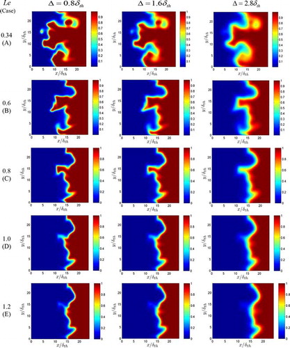
The distributions of on x₁ − x₂ mid-plane for Δ = 0.8δ_th, 1.6δ_th, and 2.8δ_th at t =1.75 t_c for cases A–E are shown in Figure 1, which shows an increase in the extent of flame wrinkling with decreasing Le. The extent of flame wrinkling can be quantified in terms of the normalized turbulent flame surface area A_T/A_L, where the flame surface area is evaluated using the volume integration of the form: A = ∫ _V|∇c|dV with subscripts “T” and “L” denoting the turbulent and laminar flame values, respectively [28]. The values of A_T/A_L and the normalized turbulent burning velocity S_T/S_L (where ) at 1.75t_c = δ_th/S_L are listed in Table 2, which demonstrates that both A_T/A_L and S_T/S_L increase significantly with decreasing Lewis number. The burning rate per unit area in turbulent flames increases (decreases) compared with the corresponding laminar value as a result of negative (positive) Markstein length [7–10] for the Le < 1 (Le > 1) flames. This, in turn, leads to S_T/S_L > A_T / A_L (S_T / S_L < A_T / A_L) in the Le < 1 (Le > 1) flames (see Table 2). It can be further seen from Figure 1 that the flame brush thickens (i.e., the magnitude of decreases) and the extent of flame wrinkling decreases with increasing Δ as a result of the smearing of local information due to the convolution operation associated with LES filtering. As the SDR is related to the reaction rate, and the gradient of the reaction progress variable, the effects of Le on burning rate and Δ dependence of are expected to influence the statistical behavior of SDR and its transport. The effects of Le and Δ on the statistical behavior of SDR and its transport have been analyzed elsewhere [28] and the current analysis will only concentrate on the influences of global Lewis number on the modeling of SDR transport.

Table 2. The effects of Lewis number on normalized flame surface area A_T/A_L and normalized turbulent flame speed S_T/S_Lwhen the statistics were extracted (i.e., t = 1.75 α_T0/).

Case	AT/AL	ST/SL
A	3.93	13.70
B	2.66	4.58
C	2.11	2.53
D	1.84	1.83
E	1.76	1.50

Figure 1. Distributions of on x₁ − x₂ mid-plane for Δ = 0.8δ_th (1st column), 1.6δ_th (2nd column), 2.8δ_th (3rd column) for cases A–E (1st–5th row) when the statistics were extracted (i.e., t = 1.75 α_T0/).

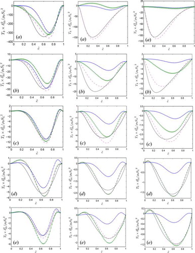
The normalized mean values of T₁, T₂, T₃, T₄, (−D₂), and f(D) conditional on for cases A–E are shown in Figure 2 for Δ ≈ 0.4δ_th and Δ ≈ 2.8δ_th. Figure 2 shows that T₂ and (−D₂) act as source and sink, respectively, in all cases, which is consistent with previous findings [21, 28]. The contribution of T₄ is positive for a major portion of the flame brush before becoming negative toward the burned gas side for Δ ≤ δ_th (e.g., Δ ≈ 0.4δ_th); however, for Δ > δ_th (e.g., Δ ≈ 2.8δ_th) the contribution of T₄ remains a leading-order source throughout the flame brush. The term T₃ assumes positive values toward the unburned gas side of the flame brush before assuming mostly negative values for the major part of the flame brush in cases D and E, whereas T₃ is negative throughout the flame brush in cases A–C for all filter widths. The contribution of f(D) is negative (positive) toward the unburned (burned) gas side of the flame brush for all cases and for all filter widths. The magnitude of T₁ is negligible compared with T₂, T₃, T₄, (−D₂), and f(D) for all Δ in all cases. It can be seen from Figure 2 that the magnitude of all the terms decrease with increasing Le and Δ, which is consistent with previous findings based on DNS data [22, 28]. The observed behaviors of T₁, T₂, T₃, T₄, (−D₂), and f(D) in response to Le and Δ have recently been explained by Gao et al. [28] using a detailed scaling analysis, and the scaling estimates of the filtered SDR and the unclosed terms of the SDR transport equation are provided in Table 3. It is worth noting that m and n in Table 3 are positive numbers with magnitudes greater than unity, and the functions g(Le), φ(Le), φ₁(Le), and Ψ(Le) increase with decreasing global Lewis number Le. It can be seen from the scaling estimates in Table 3 that the magnitudes of the terms T₁, T₂, T₃, T₄, (−D₂), and f(D) are expected to increase with decreasing filter width and global Lewis number. Interested readers are referred to [28] for further discussion on the derivation of the scaling estimates of T₁, T₂, T₃, T₄, (−D₂), and f(D), and only the modeling of these terms will be discussed in this paper in the following subsections.

Figure 2. Variations of T₁ ( —— ), T₂ (

), T₃ (

), T₄ (

), (−D₂) (

), and f(D) (

) conditionally averaged in bins of for Δ ≈ 0.4δ_th (1st column), 1.6δ_th (2nd column), and 2.8δ_th (3rd column) in cases A–E (1st–5th row). All the terms are normalized with respect to .

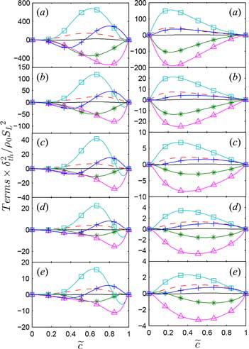
Table 3. Summary of the scaling estimates of the relevant quantities according to Gao et al. [28].

Quantities	Scaling estimates
T1	alternatively The above expressions can be combined as
T2
(T2)res (see Eq. 7ii)
T3	alternatively
(T3)res (see Eq. 11iii)
T4
(T4)res (see Eq. 14i)
(−D2)	alternatively
(−D2)res (see Eq. 14ii)
f(D)
{f(D)}res (see Eq. 14iii)

3.1. Modeling of the turbulent transport term T₁

Equation (4i) indicates that the turbulent transport term T₁ could be satisfactorily closed if the sub-grid flux of SDR (i.e., ) is properly modeled. The sub-grid flux of SDR is often modeled using a gradient hypothesis as follows [34]:

(5i)

where D_t is the sub-grid scale eddy diffusivity. It has been demonstrated earlier that the turbulent scalar flux of scalar gradients (e.g., flame surface density and SDR) may exhibit counter-gradient (gradient) transport for the flames when counter-gradient (gradient) transport is observed for [20, 22, 23, 62]. Thus, the modeling of T₁ needs to include both gradient and counter-gradient transports of .

Gao et al. [28] demonstrated that the unclosed term T₁ can be scaled in the following manner:

(5ii)

where g(Le) is a function increasing with decreasing Le, which accounts for flame normal acceleration, S_L is used to scale the sub-grid velocity fluctuations associated with sub-grid scalar gradients, and the sub-grid fluctuations of SDR are taken to scale with S_L/δ_L [28]. In Eq. (5ii), Da_Δ = ΔS_L/u′_Δδ_th and Re_Δ = ρ₀u′_ΔΔ/μ₀ are the sub-grid Damköhler number and sub-grid turbulent Reynolds number, respectively, with and being the sub-grid turbulent velocity fluctuation and sub-grid kinetic energy, respectively. One obtains Da_ΔRe_Δ ∼ (Δ/δ_th)² using μ₀ ∼ ρ₀S_Lδ_th, which indicates that Da_ΔRe_Δ increases with increasing Δ. Alternatively, one obtains the following expression when the sub-grid velocity fluctuations are taken to scale with u′_Δ [28]:

(5iii)

It is worth noting that the scaling estimate given by Eq. (5ii) (Eq. (5iii)) is more appropriate for counter-gradient (gradient) transport. Equations (5ii) and (5iii) can be combined to obtain the following scaling estimate, which is valid for both gradient and counter-gradient transport [28]:

(5iv)

Gao et al. [53] have recently extended a RANS model proposed by Chakraborty and Swaminathan [51] for the purpose of modeling for the unity Lewis number flames in the context of LES in the following manner:

(6i)

where is the ith component of the resolved flame normal vector for LES, Φ′ = 0.7 is a model parameter, and the following values have been suggested for γ₁, γ₂, and C_F [53]:

(6ii)

The parameterization given by Eq. (6ii) ensures that γ₂ assumes an asymptotic value for large values of Re_Δ (i.e., Re_Δ → ∞ ). In Eq. (6i), the first term on the right-hand side principally accounts for the effects of flame normal acceleration due to heat release, whereas the last term on the right-hand side of Eq. (6i) represents turbulent transport according to conventional gradient hypothesis. Moreover, the first and second terms on the right-hand side of Eq. (6i) are consistent with the scaling estimates given by Eqs. (5iv) and (5iii), respectively.

The predictions of according to Eq. (6i) with Φ′ = 0.7 are compared to the corresponding quantity extracted from DNS data for Δ ≈ 0.4δ_th, 1.6δ_th, and 2.8δ_th in Figure 3 for cases A–E. Figure 3 shows that even though Eq. (6i) predicts in a reasonable manner in the cases with Le ≈ 1.0 (e.g., cases C–E), this model does not adequately capture the correct qualitative and quantitative behaviors of for the flames with Le << 1.0 (i.e., cases A and B). The model given by Eqs. (6i) and (6ii) does not explicitly account for non-unity Lewis number effects, so it is not surprising that this model does not adequately capture the behavior of for Le << 1.0 flames where the nondimensional temperature T⁺ = (T − T₀)/(T_ad − T₀) is significantly different from the reaction progress variable c, which alters the distribution of heat release and thermal expansion within the flame brush compared with the Le ≈ 1.0 flames. This behavior is mimicked here by introducing Le dependence of the model parameter Φ′ in the following manner:

(6iii)

Figure 3. Variations of (

) conditionally averaged in bins of along with the predictions of Eqs. (6i) and (6ii) with Φ′ = 0.7 (

) and Eqs. (6i) and (6ii) with Φ′ according to Eq. (6iii) (

) for Δ ≈ 0.4δ_th (1st column), 1.6δ_th (2nd column), and 2.8δ_th (3rd column) in cases A–E (1st–5th row).

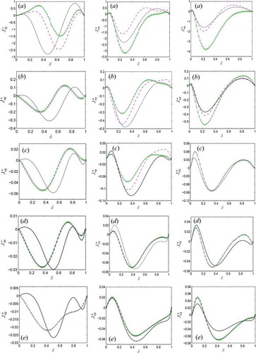
The predictions of the model given by Eq. (6i) with Φ′ according to Eq. (6iii) are also shown in Figure 3, which demonstrates that the model with new parameterization Φ′ = 0.3(1 − Le) + 0.7 predicts satisfactorily for all filter widths in all cases considered here and the agreement between the predictions of Eq. (6i) and DNS data improves with increasing Δ (see Figure 3). The predictions of Eq. (6i) with Φ′ according to Eq. (6iii) become equal to the corresponding values obtained for Φ′ = 0.7 for the Le = 1.0 case, and these two predictions cannot be distinguished from each other for case D in Figure 3. It worth noting that the sub-grid flux of the reaction progress variable (i.e., ) requires modeling in LES, and the performances of the models for and the turbulent transport term T₁ depend on the modeling of . The modeling of is beyond the scope of the current analysis and interested readers are referred to recent investigations by Chakraborty and Cant [63] and Gao et al. [64] for further discussion on the modeling of turbulent scalar fluxes in premixed turbulent flames.

3.2. Modeling of the density variation term T₂

For unity Lewis number flames the gas density ρ can be expressed as ρ₀/(1 + τc) [33], which leads to an alternative expression for the density variation term T₂ as [22, 47, 48, 51, 53]: . However, ρ = ρ₀/(1 + τT⁺) ≠ ρ₀/(1 + τc) in the non-unity Lewis number flames because the equality between T⁺ and c no longer holds. Although does not strictly hold in non-unity Lewis number flames, the gas density can still be scaled as ρ ∼ ρ₀/(1 + τc); thus, the density variation term T₂ can be scaled for adiabatic flames with low Mach number as follows [28]:

(7i)

where m is a positive number greater than unity (i.e., m > 1). The resolved part of T₂ can be taken to scale as [28]

(7ii)

where U_ref is a velocity scale representing the Favre-filtered velocity components . It is worth noting that for unity Lewis number flames yields ; however, the expression does not strictly hold for non-unity Lewis number flames, but and (T₂)_res can still be scaled using ρ₀/(1 + τ˜c) and , respectively.

The scaling estimates given by Eqs. (7i) and (7ii) demonstrate that T₂ remains of the order of irrespective of Δ. By contrast, the magnitude of (T₂)_res remains comparable to for U_ref ∼ S_L and Δ ≈ δ_th; however, the magnitude of (T₂)_res is expected to decrease with increasing Δ. This suggests that the sub-grid component (T₂)_sg = T₂ − (T₂)_res plays an increasingly important role with increasing Δ, which can be substantiated from Figure 4, where the variations of the mean values of T₂ and (T₂)_sg = T₂ − (T₂)_res conditional on are shown for cases A–E for Δ ≈ 0.4δ_th, 1.6δ_th, and 2.8δ_th.

Figure 4. Variations of T₂ (

) and (T₂)_sg (

) conditionally averaged in bins of along with the predictions of Eqs. (8) (

) and (9) (

) for Δ ≈ 0.4δ_th (1st column), 1.6δ_th (2nd column), and 2.8δ_th (3rd column) in cases A–E (1st–5th row). All the terms are normalized with respect to .

Gao et al. [53] recently proposed the following model T₂ for unity Le flames in the following manner:

(8)

where Ka_Δ = (u′_Δ/S_L)^3/2(Δ/δ_th)^−1/2 is local sub-grid Karlovitz number and is a model parameter. The first term on the right-hand side of Eq. (8) accounts for the resolved component (T₂)_res, whereas the second term models the sub-grid component. The Karlovitz number dependence in Eq. (8) ensures the diminishing strength of heat release with increasing Ka_Δ [22, 28, 47, 48, 51, 52] as the combustion process is likely to show the attributes of the broken reaction zones regime [55] (where the effects of heat release are weak) for high values of Karlovitz number. The prediction of Eq. (8) is also shown in Figure 4 for cases A–E for Δ ≈ 0.4δ_th, 1.6δ_th, and 2.8δ_th. A comparison between the predictions of Eq. (8) and the normalized T₂ extracted from explicitly filtered DNS data reveals that Eq. (8) satisfactorily predicts T₂ for a range of different filter widths for flames with Le ≈ 1.0 (e.g., cases C–E); however, this model significantly underpredicts the magnitude of T₂ for the Le << 1.0 cases (e.g., cases A and B). It can be seen from Eq. (7i) that the magnitude of T₂ is expected to increase with decreasing Le due to the strengthening of heat release effects as a result of the enhanced burning rate for the small values of Lewis number (see Table 2). As this effect is missing in Eq. (8), this model underpredicts the magnitude of T₂ for the Le << 1.0 cases (e.g., cases A and B), where the effects of enhanced heat release due to the differential diffusion of heat and mass are particularly strong.

Here the model given by Eq. (8) has been extended in order to account for the effects of Le in the following manner:

(9i)

(9ii)

In Eq. (9ii) accounts for the strengthening of heat release effects with decreasing Le as suggested by the scaling estimate given by Eq. (7i). The parameter is a thermo-chemical parameter, which provides information regarding the SDR-weighted dilatation rate [34, 36, 65, 66]. The thermo-chemical parameter accounts for the correlation between and ρN_c within the flame front. It is possible to approximate f_b(c) as f_b(c) = 1/|∇c|_L [65, 66], which enables one to evaluate from laminar flame data. The thermo-chemical parameter is also affected by Le and it is equal to 0.52, 0.67, 0.71, 0.78, and 0.79, respectively, for the Le = 0.34, 0.6, 0.8, 1.0, and 1.2 flames considered here. The predictions of Eq. (9) are compared to the predictions of Eq. (8) and T₂ extracted from DNS data in Figure 4, which shows that Eq. (9) satisfactorily predicts the quantitative behavior of T₂ for a range of different values of Δ for flames with Le ranging from 0.34 to 1.2. Eq. (9) becomes exactly equal to Eq. (8) for the Le = 1.0 case and thus the predictions of Eqs. (8) and (9) cannot be distinguished from each other for case D in Figure 4.

3.3. Modeling of the scalar turbulence interaction term T₃

The variations of the mean values of T₃ conditional on are shown in Figure 5 for cases A–E at Δ ≈ 0.4δ_th, 1.6δ_th, and 2.8δ_th. Figure 5 shows that T₃ assumes predominantly negative values throughout the flame brush for cases A–C, but this term exhibits weak positive values toward both the unburned gas sides of the flame brush before assuming mostly negative values for the major portion of the flame brush in cases D and E. The term T₃ can be expressed as follows [21, 28, 34, 45–48]:

(10)

where e_a, e_β, and e_γ are the most extensive, intermediate, and most compressive principal strain rates and their angles with∇c, respectively. Equation (10) suggests that a predominant collinear alignment of ∇c with e_a (e_γ) leads to a negative (positive) value of T₃. It was discussed elsewhere [21, 28, 34, 45–48] that ∇c predominantly aligns with e_a, when the strain rate induced by the flame normal acceleration overcomes turbulent straining, whereas one obtains preferential alignment of ∇c with e_γ when turbulent straining dominates over the strain rate due to flame normal acceleration. The flame normal acceleration strengthens with decreasing Le, and thus ∇c predominantly aligns with e_a, for the Le << 1 flames (e.g., cases A and B), leading to negative values of T₃ [21, 22, 28]. By contrast, turbulent straining overcomes the flame normal acceleration on both ends of the flame brush for the Le ≈ 1.0 cases considered here (e.g., cases C–E), which leads to positive values of T₃ both on unburned and on burned gas sides of the flame brush for Δ ≈ 0.4δ_th. However, the flame normal acceleration dominates over turbulent straining in the middle of the flame brush where the effects of heat release are strong even in the Le ≈ 1.0 cases considered here (e.g., cases C–E), which leads to negative values of T₃ for the major portion of the flame brush in these cases.

Figure 5. Variations of T₃ (

) and (T₃)_res (

) conditionally averaged in bins of along with the predictions of Eqs. (12i) and (12iii) (

) and Eqs. (13i) and (13ii) (

) for Δ ≈ 0.4δ_th (1st column), Δ ≈ 1.6δ_th (2nd column), and Δ ≈ 2.8δ_th (3rd column) in cases A–E (1st–5th row). All the terms are normalized with respect to .

The effects of ∇c alignment with e_a, on T₃ can be scaled in the following manner [28]:

(11i)

The contribution of ∇c alignment with e_γ on T₃ can be scaled as follows [28]:

(11ii)

The Lewis number Le dependence in Eq. (11i) (with n > 1) accounts for the greater extent of ∇c alignment with e_a for the flames with Le << 1.0. Gao et al. [28] proposed the following scaling estimate of the resolved part of T₃:

(11iii)

A comparison of Eqs. (11i)–(11iii) reveals that the contribution of (T₃)_res to T₃ is expected to weaken with increasing Δ, and this behavior can indeed be seen from Figure 5, which shows that the magnitude of (T₃)_res decreases with increasing Δ.

Gao et al. [53] utilized the scaling estimates given by Eqs. (11i) and (11ii) to propose a model for T₃ for Le = 1.0 flames:

(12i)

where C₃ and C₄ are the model parameters and is the density-weighted local sub-grid Damköhler number. The symbol is a bridging function in terms of ΔS_L/α_T0, which ensures that (T₃)_sg ≈ T₃ for Δ >> δ_th and T₃ approaches (T₃)_res when the flow is fully resolved:

(12ii)

Gao et al. [53] proposed the following expressions for the model parameter C₃, C₄, and :

(12iii)

It is worth noting that the terms and are consistent with scaling estimates given by Eqs. (11i) and (11ii), respectively. However, a comparison between Eq. (11i) and reveals that the increased alignment of ∇c with e_α for small values of Le as a result of the strengthening of flame normal acceleration is not accounted for by the model given by Eq. (12ii). The effects of flame normal acceleration are expected to weaken with increasing Karlovitz number as the reacting flow field exhibits some attributes of passive scalar mixing for large values of Karlovitz number in the broken reaction zones regime [55]. This behavior is mimicked here by Ka_Δ dependence of C₄in Eq. (12iii).

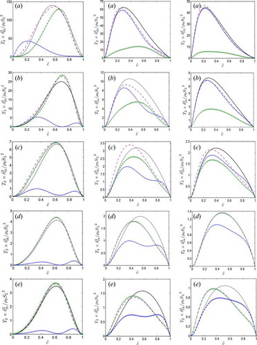
The predictions of Eq. (12i) with the model parameters given by Eq. (12ii) are compared to T₃ extracted from DNS data in Figure 5, which shows that Eq. (12i) adequately captures the qualitative and quantitative behaviors of T₃ for the Le ≈ 1.0 cases considered here (e.g., cases C–E); however, this model has been found to underpredict the magnitude of the negative contribution of T₃ in the Le << 1.0 cases (e.g., cases A and B) for Δ > δ_th. It has already been noted that the increased extent of scalar gradient destruction in the Le << 1.0 flames, due to the preferential alignment of ∇c with e_α under strong actions of flame normal acceleration, is not addressed in the model given by Eq. (12i). Thus, this model underpredicts the negative contribution of T₃ for the flames with Le << 1.0. Here Eq. (12i) has been modified in the following manner to account for non-unity Lewis number effects:

(13i)

(13ii)

The involvement of the function Γ(Le) in Eq. (13i) accounts for the strengthening of ∇c alignment with e_α under strong actions of flame normal acceleration in flames with small values of Lewis number. The presence of helps Eq. (13i) capture the qualitative behavior of T₃ across the flame brush. It can be seen from Figure 5 that the model given by Eq. (13i) provides satisfactory qualitative and quantitative predictions of T₃ for all the flames with different values of Le for a range of Δ. It is worth noting that Eq. (13i) approaches Eq. (12i) for Le = 1.0 and thus the predictions of Eqs. (12i) and (13i) cannot be distinguished from each other for case D in Figure 5.

3.4. Modeling of the combined reaction, dissipation, and diffusivity gradient contribution [T₄ − D₂ + f(D)]

The variations of the mean values of [T₄ − D₂ + f(D)] conditional on are shown in Figure 6 for A–E for Δ ≈ 0.4δ_th, 1.6δ_th, and 2.8δ_th. It can be seen from Figure 6 that [T₄ − D₂ + f(D)] acts as a sink (source) term toward the burned (unburned) gas side of the flame brush for Δ ≈ 0.4δ_th and Δ ≈ 1.6δ_th; however, the mean value of [T₄ − D₂ + f(D)] conditional on assumes predominantly negative values for Δ ≈ 2.8δ_th. Table 3 shows that the order of magnitudes of T₄, (−D₂), and f(D) remain comparable according to the scaling analysis by Gao et al. [28] and their magnitudes are expected to increase with decreasing Le. Furthermore, the scaling estimates of (T₄)_res, (−D₂)_res, and {f(D)}_res in Table 3 suggest that their contributions are expected to weaken with increasing Δ, where (T₄)_res, (−D₂)_res, and {f(D)}_res are the resolved components of T₄, (−D₂), and f(D), which are given by

(14i)

(14ii)

(14iii)

Figure 6. Variations of [T₄ + f(D) − D₂] (

) and [(T₄)_sg − (D₂)_sg + {f(D)}_sg] (

) conditionally averaged in bins of along with the predictions of Eqs. (15i) and (15ii) (

) and Eq. (16) (

) for Δ ≈ 0.4δ_th (1st column), 1.6δ_th (2nd column), and 2.8δ_th (3rd column) in cases A–E (1st–5th row). All the terms are normalized with respect to .

Thus, the sub-grid components (T₄)_sg = T₄ − (T₄)_res, (−D₂)_sg = −D₂ + (D₂)_res, and {f(D)}_sg = f(D) − {f(D)}_res are expected to play major roles for Δ >> δ_th. The aforementioned behaviors of the resolved and sub-grid components of T₄, (−D₂), and f(D) can be confirmed from Figure 6. It can be seen from Table 3 that the magnitudes of (T₄)_sg, (−D₂)_sg, and {f(D)}_sg remain of the order of for Δ >> δ_th; however, their magnitudes are expected to increase with decreasing Le, which can indeed be substantiated from Figure 6.

Gao et al. [53] utilized to model [T₄ + f(D) − D₂] together for unity Lewis number flames by extending an existing RANS model [22, 34, 44, 47, 48, 51] in the following manner:

(15i)

(15ii)

The involvement of in Eq. (15i) is required for capturing the qualitative behavior of [T₄ − D₂ + f(D)] across the flame brush, whereas f_TD approaches unity for small values of Δ as the terms get fully resolved (i.e., ). The transition from positive to negative contribution of [T₄ + f(D) − D₂] with increasing Δ has been accounted for by . The predictions of Eq. (15i) are shown in Figure 6, which shows that this model captures both the qualitative and quantitative behaviors of [T₄ + f(D) − D₂] for the Le ≈ 1.0 cases considered here (e.g., cases C–E); however, this model underpredicts the magnitude of [T₄ + f(D) − D₂] significantly for the Le << 1.0 cases (e.g., cases A and B). It is worth noting that the model given by Eq. (15i) does not account for the increased magnitude of {T₄ − D₂ + f(D)}_sg for small values of Le (see Table 3); hence, perhaps it is not surprising that this model under-predicts the magnitude of [T₄ + f(D) − D₂] for the flames with Le << 1.0 (e.g., cases A and B). The increased magnitude of [T₄ + f(D) − D₂] for the small values of Le is accounted for by modifying Eq. (15i) in the following manner:

(16)

where and f_TD are considered according to Eq. (15ii). The predictions of Eq. (16) are shown in Figure 6, which demonstrates that Eq. (16) captures both the qualitative and quantitative behaviors of [T₄ + f(D) − D₂] for a range of filter widths for different Le cases considered here. Equations (15i) and (16) become equal to each other for Le = 1.0 and thus their predictions cannot be separated from each other in case D in Figure 6.

It is worth noting that the combined contribution of the terms D₁, T₄, f(D), and (−D₂) can be expressed in the following manner if the SDR transport equation is derived based on the kinematic form of the progress variable transport equation (i.e., Dc/Dt = S_d|∇c|) [34, 47]:

(17)

where and are the flame displacement speed and local flame normal vector, respectively. Thus, Eq. (17) suggests that the net contribution of [T₄ − D₂ + f(D)] originates due to flame normal propagation and flame curvature. This justifies the modeling of these terms together [21, 34, 44, 47, 48, 53] because the molecular diffusion term D₁ is a closed term. Although Eq. (16) reasonably captures the qualitative behavior and the magnitude of [T₄ + f(D) − D₂] for all cases considered here, the collective modeling of the terms T₄, f(D), and (−D₂) may give rise to the loss of their individual physical significances. However, this is one of the first attempts to model the Lewis number effects on the SDR transport equation terms in the context of LES of premixed combustion and thus there is a scope for further improvement of this modeling in the future.

3.5. Implications of model implementation

The newly proposed models for the unclosed terms of the SDR transport equation are summarized in Table 4 for the future potential users of these models. It is worth noting that the flamelet assumption is invoked while deriving these models, so they are expected to remain valid in the corrugated flamelets and thin reaction zones regimes of turbulent premixed combustion [55]. The scaling estimates in Table 3 indicate that the terms T₂, T₃, T₄, (−D₂), and f(D) remain leading-order contributors to the SDR transport and the magnitude of T₁ remains negligible compared with the terms T₂, T₃, T₄, (−D₂), and f(D) irrespective of Damköhler and turbulent Reynolds numbers. This is consistent with the observations made from Figure 2. However, the turbulent transport term T₁ still needs to be modeled and included in the model implementation for LES for numerical stability.

Table 4. Summary of the proposed models for the unclosed terms of the SDR transport equation (Eq. (3)) in this analysis.

Term	Model expression
	where γ1 = 1.8, γ2 = 4.9 − 3.2erf(0.15RetΔ), RetΔ = ρ0u′ΔΔ/μ0, Φ = 0.3(Le − 1) + 0.7 and CF = 0.11
T2	where KaΔ = (u′Δ/SL)^3/2(Δ/δth)^−1/2 is local sub-grid Karlovitz number and .
T3	where C3 = 7.5, C4 = 0.75(1.0 + KaΔ)^−0.4, and with p = 0.2 + 1.5(1 − Le)
[T4 − D2 + f(D)]	where fTD = exp[−0.27(SLΔ/αT0)^1.7], c* = 1.0 − 0.83erf[0.5(ΔSL/αt0) − 2.3] and β′3 = 5.7/Le^0.2

4. Conclusions

The effects of global Lewis number Le on the modeling of the unclosed terms of the transport equation of Favre-filtered SDR have been analyzed based on a priori analysis of a DNS database of freely propagating statistically planar turbulent premixed flames with Le ranging from 0.34 to 1.2. It has been found that Le has profound influence on the statistical behavior of the unclosed terms of transport arising from turbulent transport T₁, density variation due to heat release T₂, alignment of scalar and velocity gradients T₃, correlation between the gradients of reaction rate and reaction progress variable T₄, molecular dissipation (−D₂), and diffusivity gradients f(D), and detailed physical explanations have been provided for the observed non-unity Lewis number effects. Recently proposed models for T₁, T₂, T₃, T₄, (−D₂), and f(D) for unity Lewis number flames have been extended here to account for the effects of Le based on the scaling estimates of these unclosed terms [28]. The newly proposed models have been found to satisfactorily predict the unclosed terms obtained from explicitly filtered DNS data for a range of Δ for different values of Le. However, it is still essential to implement these models into actual LES simulations for the purpose of a posteriori assessment. Moreover, these models need to be further validated based on detailed chemistry-based DNS simulations. Further validation of these models will form the basis of future investigations.

References

- Y. Huang and V. Yang, Dynamics and Stability of Lean-Premixed Swirl Stabilised Combustion, Prog. Energy Combust. Sci., vol. 35, no. 4, pp. 293–364, 2009.
- T. Wallner, H. K. Ng, and R. W. Peters, The Effects of Blending Hydrogen with Methane on Energy Operation, Efficiency and Emissions, Proc. SAE Trans., 2007–01-0474, 2007.
- R. Schefer, Reduced Turbine Emissions Using Hydrogen-Enriched Fuels, Proc. of the 2002 U.S. DOE Hydrogen Program Review NREL/CP-610–32405, 2002.
- M. Mizomoto, S. Asaka, S. Ikai, and C. K. Law, Effects of Preferential Diffusion on the Burning Intensity of Curved Flames, Proc. Combust. Inst., vol. 20, pp. 1933–1939, 1984.
- C. K. Law and O. C. Kwon, Effects of Hydrocarbon Substitution on Atmospheric Hydrogen–Air Flame Propagation, Int. J. Hydrogen Energy, vol. 29, pp. 867–879, 2004.
- F. Dinkelacker, B. Manickam, and S. R. Mupppala, Modelling and Simulation of Lean Premixed Turbulent Methane/Hydrogen/Air Flames with an Effective Lewis Number Approach, Combust. Flame, vol. 158, pp. 1742–1749, 2011.
- P. Pelce and P. Clavin, Influence of Hydrodynamics and Diffusion Upon the Stability Limits of Laminar Premixed Flames, J. Fluid Mech., vol. 124, pp. 219–237, 1982.
- P. Clavin and F. A. Williams, Effects of Molecular Diffusion and Thermal Expansion on the Structure and Dynamics of Turbulent Premixed Flames in Turbulent Flows of Large Scale and Small Intensity, J. Fluid Mech., vol. 128, pp. 251–282, 1982.
- P. A. Libby, A. Linan, and F. A. Williams, Strained Premixed Laminar Flames with Non-Unity Lewis Numbers, Combust. Sci. Technol., vol. 34, pp. 257–293, 1983.
- G. I. Sivashinsky, Instabilities, Pattern Formation and Turbulence in Flames, Annu. Rev. Fluid Mech., vol. 15, pp. 179–190, 1983.
- R. G. Abdel-Gayed, D. Bradley, M. Hamid, and M. Lawes, Lewis Number Effects on Turbulent Burning Velocity, Proc. Combust. Inst., vol. 20, pp. 505–512, 1984.
- W. T. Ashurst, N. Peters, and M. D. Smooke, Numerical Simulation of Turbulent Flame Structure with Non-Unity Lewis Number, Combust. Sci. Technol., vol. 53, pp. 339–375, 1987.
- D. Haworth and T. J. Poinsot, Numerical Simulations of Lewis Number Effects in Turbulent Premixed Flames, J. Fluid Mech., vol. 244, pp. 405–436, 1992.
- C. J. Rutland and A. Trouvé, Direct Simulations of Premixed Turbulent Flames with Nonunity Lewis Numbers, Combust. Flame, vol. 94, pp. 41–57, 1993.
- A. Trouvé and T. J. Poinsot, The Evolution Equation for Flame Surface Density in Turbulent Premixed Combustion, J. Fluid Mech., vol. 278, pp. 1–31, 1994.
- N. Chakraborty, and R. S. Cant, Influence of Lewis Number on Curvature Effects in Turbulent Premixed Flame Propagation in the Thin Reaction Zones Regime, Phys. Fluids, vol. 17, 105105, 2005.
- J. Yuan, Y. Ju, and C. K. Law, Coupled Hydrodynamic, and Diffusional Thermal Instabilities in Flame Propagation at Small Lewis Numbers, Phys. Fluids, vol. 17, 074106, 2005.
- N. Chakraborty and M. Klein, A Priori Direct Numerical Simulation Assessment of Algebraic Flame Surface Density Models for Turbulent Premixed Flames in the Context of Large Eddy Simulation. Phys. Fluids, vol. 20, 085108, 2008.
- I. Han and K. H. Huh, Roles of Displacement Speed on Evolution of Flame Surface Density for Different Turbulent Intensities and Lewis Numbers in Turbulent Premixed Combustion, Combust. Flame, vol. 152, pp. 194–205, 2008.
- N. Chakraborty, and R. S. Cant, Effects of Lewis Number on Scalar Transport in Turbulent Premixed Flames, Phys. Fluids, vol. 21, 035110, 2009.
- N. Chakraborty, M. Klein, and N. Swaminathan, Effects of Lewis Number on Reactive Scalar Gradient Alignment with Local Strain Rate in Turbulent Premixed Flames, Proc. Combust. Inst., vol. 32, pp. 1409–1417, 2009.
- N. Chakraborty and N. Swaminathan, Effects of Lewis Number on Scalar Dissipation Transport and Its Modelling Implications for Turbulent Premixed Combustion, Combust. Sci. Technol., vol. 182, pp. 1201–1240, 2010.
- N. Chakraborty and R. S. Cant, Effects of Lewis Number on Flame Surface Density Transport in Turbulent Premixed Combustion, Combust. Flame, vol. 158, pp. 1768–1787, 2011.
- N. Chakraborty, M. Katragadda, and R. S. Cant, Effects of Lewis Number on Turbulent Kinetic Energy Transport in Turbulent Premixed Combustion, Phys. Fluids, vol. 23, 075109, 2011.
- N. Chakraborty, and N. Swaminathan, Effects of Lewis Number on Scalar Variance Transport in Turbulent Premixed Flames, Flow, Turb. Combust., vol. 87, nos. 2–3, pp. 261–292, 2011.
- N. Chakraborty, and A. N. Lipatnikov, Effects of Lewis Number on the Statistics of Conditional Fluid Velocity in Turbulent Premixed Combustion in the Context of Reynolds Averaged Navier Stokes Simulations, Phys. Fluids, vol. 25, 045101, 2013.
- N. Chakraborty, L. Wang, and M. Klein, Effects of Lewis Number on Streamline Segment Analysis of Turbulent Premixed Flames, Phys. Rev. E, vol. 89, 033015, 2014.
- Y. Gao, N. Chakraborty, and N. Swaminathan, Scalar Dissipation Rate Transport in the Context of Large Eddy Simulations for Turbulent Premixed Flames with Non-Unity Lewis Number, Flow Turb. Combust., vol. 93, pp. 461–486, 2014.
- R. W. Bilger, Some Aspects of Scalar Dissipation, Flow Turb. Combust., vol. 72, pp. 93–114, 2004.
- R. O. Fox, Computational Models for Turbulent Reacting Flow, Cambridge University Press, Cambridge, UK, 2003.
- N. Kasagi, Y. Tomita, and A. Kuroda, Direct Numerical Simulation of Passive Scalar Field in a Turbulent Channel Flow, J. Heat Transfer, vol. 114, no. 3, pp. 598–606, 2008.
- S. C. P. Cheung, G. H. Yeoh, A. L. K. Cheung, R. K. K. Yuen, and S. M. Lo, Flickering Behaviour of Turbulent Fires Using Large Eddy Simulation, Numer. Heat Trans. A., vol. 52, no. 7, pp. 679–712, 2007.
- K. N. C. Bray, Turbulent Flows with Premixed Reactants, in P. A. Libby, and F. A. Williams, (eds.), Turbulent Reacting Flows, Springer Verlag, Berlin Heidelburg, New York, pp. 115–183, 1980.
- N. Chakraborty M. Champion A. Mura, and N. Swaminathan, Scalar Dissipation Rate Approach to Reaction Rate Closure, in N. Swaminathan, and K. N. C. Bray, (eds.), Turbulent Premixed Flame, 1st ed., Cambridge University Press, Cambridge, UK, pp. 76–1023, 2011.
- S. P. Malkeson and N. Chakraborty, The Modeling of Fuel Mass Fraction Variance Transport in Turbulent Stratified Flames: A Direct Numerical Simulation Study, Numer. Heat Trans. A., vol. 58, no. 3, pp. 187–206, 2010.
- T. Dunstan, Y. Minamoto, N. Chakraborty, and N. Swaminathan, Scalar Dissipation Rate Modelling for Large Eddy Simulation of Turbulent Premixed Flames, Proc. Combust. Inst., vol. 34, pp. 1193–1201, 2013.
- Y. Gao, N. Chakraborty, and N. Swaminathan, Algebraic Closure of Scalar Dissipation Rate for Large Eddy Simulations of Turbulent Premixed Combustion, Combust. Sci. Technol., vol. 186, pp. 1309–1337, 2014.
- T. Ma, Y. Gao, A. M. Kempf, and N. Chakraborty, Validation and Implementation of Algebraic LES Modelling of Scalar Dissipation Rate for Reaction Rate Closure in Turbulent Premixed Combustion, Combust. Flame, vol. 161, pp. 3134–3153, 2014.
- M. S. Raju, Application of Scalar Monte-Carlo Probability Density Function Method for Turbulent Spray Flames, Numer. Heat Trans. A, vol. 30, no. 8, pp. 753–777, 1996.
- Y. Pei, E. R. Hawkes, and S. Kook, Transported Probability Density Function Modelling of the Vapour Phase of an n-Heptane Jet at Diesel Engine Conditions, Proc. Combust. Inst., vol. 34, pp. 3039–3047, 2013.
- Y. Pei, E. R. Hawkes, and S. Kook, A Comprehensive Study of Effects of Mixing, and Chemical Kinetic Models on Predictions of n-Heptane Jet Ignitions with the PDF Method, Flow, Turb. Combust., vol. 91, pp. 249–280, 2013.
- T. Mantel and R. Borghi, New Model of Premixed Wrinkled Flame Propagation Based on a Scalar Dissipation Equation, Combust. Flame, vol. 96, no. 4, pp. 443–457, 1994.
- A. Mura and R. Borghi, Towards an Extended Scalar Dissipation Equation for Turbulent Premixed Combustion, Combust. Flame, vol. 133, pp. 193–196, 2003.
- N. Swaminathan and K. N. C. Bray, Effect of Dilatation on Scalar Dissipation in Turbulent Premixed Flames, Combust. Flame, vol. 143, pp. 549–565, 2005.
- N. Chakraborty, and N. Swaminathan, Influence of Damköhler Number on Turbulence-Scalar Interaction in Premixed Flames, Part I: Physical Insight, Phys. Fluids, vol. 19, 045103, 2007.
- N. Chakraborty, and N. Swaminathan, Influence of Damköhler Number on Turbulence-Scalar Interaction in Premixed Flames, Part II: Model Development, Phys. Fluids, vol. 19, 045104, 2007.
- N. Chakraborty, J. W. Rogerson, and N. Swaminathan, A Priori Assessment of Closures for Scalar Dissipation Rate Transport in Turbulent Premixed Flames Using Direct Numerical Simulation, Phys. Fluids, vol. 20, 045106, 2008.
- N. Chakraborty, J. W. Rogerson, and N. Swaminathan, The Scalar Gradient Alignment Statistics of Flame Kernels and Its Modelling Implications for Turbulent Premixed Combustion, Flow Turb. Combust., vol. 85, pp. 25–55, 2010.
- A. Mura, K. Tsuboi, and T. Hasegawa, Modelling of the Correlation between Velocity and Reactive Scalar Gradients in Turbulent Premixed Flames based on DNS Data. Combust. Theor. Modell., vol. 12, pp. 671–698, 2008.
- A. Mura, V. Robin, M. Champion, and T. Hasegawa, Small-Scale Features of Velocity and Scalar Fields of Turbulent Premixed Flames, Flow Turb. Combust., vol. 82, pp. 339–358, 2009.
- N. Chakraborty and N. Swaminathan, Effects of Turbulent Reynolds Number on the Scalar Dissipation Rate Transport in Turbulent Premixed Flames in the Context of Reynolds Averaged Navier Stokes Simulations, Combust. Sci. Technol., vol. 185, pp. 676–709, 2013.
- E. Knudsen, E. S. Richardson, E. M. Doran, H. Pitsch, and J. H. Chen, Modeling Scalar Dissipation, and Scalar Variance in Large Eddy Simulation: Algebraic, and Transport Equation Closures, Phys. Fluids, vol. 24, 055103, 2012.
- Y. Gao, N. Chakraborty, and N. Swaminathan, Scalar Dissipation Rate Transport and Its Modelling for Large Eddy Simulations of Turbulent Premixed Combustion, Combust. Sci. Technol., vol. 187, no. 3, pp. 362–383, 2015.
- J. H. Chen, A. Choudhary, D. De Supinski, E. R. Hawkes, S. Klasky, W. K. Liao, K. L. Ma, J. Mellor-Crummey, N. Podhorski, R. Sankaran, S. Shende, and C. S. Yoo, Terascale Direct Numerical Simulations of Turbulent Combustion using S3D, Comput. Sci. Discov., vol. 2, no. 1, 015001, 2009.
- N. Peters, Turbulent Combustion, Cambridge University Press, Cambridge, UK, 2000.
- K. W. Jenkins and R. S. Cant, DNS of Turbulent Flame Kernels, in C. Liu, L. Sakell, and T. Beautner, (eds.), Proc. Second AFOSR Conf. on DNS and LES, Kluwer Academic Publishers, New Brunswick, NJ, pp. 191–202, 1999.
- M. Boger, D. Veynante, H. Boughanem, and A. Trouvé, Direct Numerical Simulation Analysis of Flame Surface Density Concept for Large Eddy Simulation of Turbulent Premixed Combustion, Proc. Combust. Inst., vol. 27, pp. 917–925, 1998.
- F. Charlette, C. Meneveau, and D. Veynante, A Power-Law Flame Wrinkling Model for LES of Premixed Turbulent Combustion. Part I: Non-Dynamic Formulation and Initial Tests, Combust. Flame, vol. 131, pp. 159–180, 2002.
- R. W. Grout, An Age-Extended Progress Variable for Conditioning Reaction Rates, Phys. Fluids, vol. 19, 105107, 2007.
- H. Reddy, and J. Abraham, Two-Dimensional Direct Numerical Simulation Evaluation of the Flame Surface Density Model for Flames Developing from an Ignition Kernel in Lean Methane/Air Mixtures Under Engine Conditions, Phys. Fluids, vol. 24, 105108, 2012.
- C. Pera, S. Chevillard, and J. Reveillon, Effects of Residual Burnt Gas Heterogeneity on Early Flame Propagation and on Cyclic Variability in Spark-Ignited Engines, Combust. Flame, vol. 160, pp. 1020–1032, 2013.
- D. Veynante, A. Trouvé, K. N. C. Bray, and T. Mantel, Gradient and Countergradient Turbulent Scalar Transport in Turbulent Premixed Flames, J. Fluid Mech., vol. 332, pp. 263–293, 1997.
- N. Chakraborty and R. S. Cant, Effects of Turbulent Reynolds Number on Turbulent Scalar Flux Modelling in Premixed Flames using Reynolds Averaged Navier-Stokes Simulations, Numer. Heat Trans. A, vol. 67, no. 11, pp. 1187–1207, 2015.
- Y. Gao, N. Chakraborty, and M. Klein, Assessment of the Performances of Sub-Grid Scalar Flux Models for Premixed Flames with Different Global Lewis Numbers: A Direct Numerical Simulation Analysis, Int. J. Heat Fluid Flow, vol. 52, pp. 28–39, 2015.
- H. Kolla, J. Rogerson, N. Chakraborty, and N. Swaminathan, Prediction of Turbulent Flame Speed using Scalar Dissipation Rate, Combust. Sci. Technol., vol. 181, pp. 518–535, 2009.
- J. W. Rogerson and N. Swaminathan, Correlation between Dilatation and Scalar Dissipation in Turbulent Premixed Flames, Proc. 3rd European Combustion Meeting Crete, China, Greece, 11th to 13th April, 2007.