Inquiry-Based Modeling of Population Dynamics With Logistic Differential and Difference Equations

Abstract

Following a modeling-first approach to differential equations, inquiry-based learning activities on modeling and controlling the growth of locally relevant species, such as lionfish or sea turtles, are developed by the authors. Emerging exemplary practices are presented, building towards a balanced teaching of differential equations involving multiple mathematical perspectives, representations, and intra-disciplinary and interdisciplinary mathematical connections. This innovative approach is an effort towards realizing the MAA’s Common Vision for Undergraduate Mathematical Sciences programs in 2025. Discrete and continuous approaches are used simultaneously, while numerical and graphical methods are used to build connections between logistic differential and difference equation models. The resulting chaotic behavior of the solutions is also emphasized. We suggest that this enhancement of the Doing the Math phase of modeling outlined in SIAM’s 2016 Guidelines for Assessment and Instruction in Mathematical Modeling offers a wider access to deeper mathematics, and helps to foster complementary disciplinary perspectives in mathematics.

Keywords:

• Inquiry-based modeling
• differential equations
• difference equations
• population dynamics
• logistic growth

1. MOTIVATION

Calls for a stronger emphasis on mathematical modeling at all stages of mathematical development have been made by the leading professional organizations in mathematics, mathematical sciences, and mathematics education [17, 21, 24, 30]. With reform efforts underway, undergraduate programs in the mathematical sciences have been urged to meet the emerging demands for collaboration with other STEM and non-STEM fields. To this point, the National Research Council (NRC), the Society of Industrial and Applied Mathematics (SIAM), and the National Council for Teachers of Mathematics (NCTM), have endorsed a mathematics teaching that better aligns with other disciplines [17, 24, 30]. Furthermore, the Mathematical Association of America (MAA) has encouraged increasing the connectivity of the various mathematical sciences, in particular, by employing both analytic and computational approaches, a common sentiment echoed by the NRC and others [21].

Deeply interwoven into the modeling process is student inquiry, with inquiry-based methods in undergraduate mathematics known to be effective by both researchers and practitioners [11, 29]. Inquiry-based approaches have been offered in the learning of differential equations in response to student difficulties, with an emphasis on continuous methods [28, 29, 32]. In this paper, we discuss how we use the mathematical modeling process in differential equations as an integrative tool, connecting mathematics with a wide body of ideas from other sciences. We use the theme of population dynamics, which has natural connections across mathematics, biology, ecology, economics, etc., as thread to build these intra-disciplinary and interdisciplinary connections. Adopting a fallibilistic orientation (see [10]) to mathematics and mathematical modeling, we simultaneously present problems from multiple mathematical standpoints, allowing both students and teachers to experience the modeling process as both mathematicians and scientists.

The inquiry-based learning modules described here utilize both differential and difference equations and emphasize both discrete and continuous approaches. From each approach, students experience multiple opportunities to explore various representations: numerical, algebraic, verbal, and graphical. By using both discrete and continuous data, students are expected to experience a deeper and richer understanding of their models, and to develop broad interdisciplinary perspectives, thus realizing the common visions mentioned above.

2. BACKGROUND AND SETTING

The learning modules described in Sections 3–5 fit naturally in an introductory course on differential equations, but they can also be used in calculus, or in any course for which calculus is a prerequisite. The collection of activities, including the relevant assessments, take approximately 10 75-minute class sessions over a 5-week period. A modeling first approach is used here to connect and coordinate content, and to provide deep, rich coverage of logistic growth modeling by using both differential and difference equations in an integrated and innovative way. Portions of the inquiry-based learning modules have been implemented at the University of the Virgin Islands by the authors every semester from Fall 2015 to Summer 2017 as a part of a National Science Foundation funded project to innovate STEM Education [9]. Locally relevant population dynamics were previously emphasized at the University of the Virgin Islands by Dance and Sandefur with endangered queen conch as the pertinent species, albeit at the college algebra level [5].

Adopting a balanced practice with both discrete and continuous methods, we developed inquiry-based learning modules on growth modeling as a thread across precalculus, discrete mathematics, and calculus, including differential equations while students learn ideas such as rates of change, differentiation, initial value problems, and integration [8]. In our precalculus module, students model the spread of disease by generating numerical data with an exponential growth pattern, then proceed to analyze real data from an outbreak (Ebola), using regression methods to discover logistic growth curves in the form. $$P\left(t\right)=\frac{A}{1+B^t}.$$

We highlight numerical techniques as they come up with models using computers and calculators as available, and they experiment with their model using both discrete and continuous techniques before being presented the continuous function. Various inquiry-based learning modules have been developed by the authors including numerical and algorithmic approaches as well as visual representations of integral curves as solutions of ordinary differential equations [7, 25].

When students are early in the calculus sequence, we have them focus on the discretization of continuous variables by modeling the rates of changes of growth curves. They explore the population change in endangered sea turtles using real data from nearby Buck Island (such as that found at www.seaturtlestatus.org and [15, 16]), informing their adaptive management strategies in a local and global context. For instance, students might approximate that the sea turtle population increases by 5% each year, and discover the recursive relation $\Delta P=P_{n+1}-P_n=0.05·P_n.$

The basic idea with discrete methods in solving differential equations begins with the discretization of the domain at successive time points [26, 27]. As their study of differential equations intensifies, we have students develop difference equations that approximate differential equations in terms of a discrete function involving differences in the function values, without using any derivatives. Numerical methods are then used to build approximate solutions using their recurrence equations.

Later in the calculus sequence, the discrete approach offers students a numerical method whereby difference equations are developed from ordinary differential equations and recurrently expressed in the form of $y\prime =f(y)$. Graphical representations as a solution strategy are heavily integrated, using slope fields and available technologies, such as GeoGebra [18]. Students learn how to plot any slope field and accompanying graphical solutions for any $y\prime =f(x,y)$ [25].

3. MODELING LIONFISH POPULATION

Our activity starts after students have seen both Verhulst’s differential logistic equation, (1) $$\frac{dP}{dt}=rP\left(t\right)\left(1-\frac{P\left(t\right)}{K}\right),$$(1) and a corresponding difference equation representing logistic growth, $$\Delta P=P_{n+1}-P_n=r{P}_n-\frac{r}{K}{P}_n^2.$$

We launch with a real-world ill-posed problem:

Invasive lionfish have entered the Caribbean and are being sighted with increasing frequency in the coastal waters surrounding St. Croix. This poses a severe danger for the ecosystem and the affected coral reefs. To help prevent an ecological crisis, we need to create a mathematical model of the lionfish population that can be used to help manage this problem.

Having students work in small groups, we explain that they will receive no additional data and that they must be able to defend their assumptions in building their model, enhancing their sense of ownership of their model. Although students can freely use difference equations, they have (almost exclusively) began with the analytic approach, which requires them to know the constants used in Verhulst’s equation (1)(1) $$\frac{dP}{dt}=rP\left(t\right)\left(1-\frac{P\left(t\right)}{K}\right),$$(1) .

3.1. Initial Phases of Modeling: Setting Assumptions, Selecting Variables, Formulating

In the initial phases of modeling, we create opportunities for students to develop interdisciplinary perspectives and engage them in enhanced critical thinking; an essential 21st-century skill connected to learning across subjects and disciplines. Students need to understand the problem in context before determining a viable set of assumptions, which requires student research. We try to ensure that they tap into our local community/faculty experts that conduct research on lionfish, in addition to the usual online sources.

Students first must investigate a few questions. How many lionfish do we have here? How fast is the population of lionfish increasing? What is the carrying capacity of lionfish in our waters? Answering these questions are in fact mathematical modeling problems in themselves that require statistical methods.

As a sample of student approach (and offering no remark on the veracity of this approach), one group, after an online search, referenced Figure 1, which illustrates the abundance of lionfish sightings in nearby Bermuda.

Figure 1. Abundance of lionfish sightings, Bermuda [14].

Students reasoned that carrying capacity was reached in 2008 for Bermuda. After doing their own research, students found a second study [1] detailing the capture and tagging of 161 lionfish, with 24% recaptured. They then derived $161/0.24\approx 670$ as an estimate for the total population of lionfish in Bermuda.

To estimate the intrinsic growth rate, students entered the differential equation $$\frac{dy}{dx}=ry\left(1-\frac{y}{670}\right)$$ into a slope-field generator and experimented with varying values of r until a slope field with a solution resembling Figure 1 was obtained. Other groups obtained different parameters. Imperative to the process is discussion, reflection, and peer presentation of their graphical representations (slope fields) and symbolic representation (equations). Some assumptions embedded in the process that students did not recognize on their own came to light such as: Is St. Croix the same size as Bermuda? This gives students an early opportunity to iterate and revise.

After revisiting their initial assumptions, and citing a faculty lionfish expert whom suggested that tag/release methods underestimate the actual population, our sample group used the logistic differential equation with r = 0.8 and capacity of 850 to represent their estimation of the population after x years, with accompanying slope field shown in Figure 2.

Figure 2. Screenshot of lionfish population growth path visually traced using slope field generators. Generated by the tool Desmos [6].

4. MODELING MATHEMATICS IN POPULATION DYNAMICS CONTEXT: ALTERNATIVE METHODS FOR DOING THE MATH

4.1. Global Analytic Solutions to Differential Equations

At this point, we test students’ model by asking questions like: If x lionfish were spotted by a diving expedition, what does your model suggest? With an initial value, students generate a local graphical solution; but we require a global solution. The option to which all of our students turned is to attempt to solve the initial value problem analytically: $$\frac{dy}{dx}=ry\left(1-\frac{y}{K}\right),\hspace{1em}y\left(0\right)=\alpha$$

We find that this traditional content is often not accessible to many students. An analytic solution for equation (1)(1) $$\frac{dP}{dt}=rP\left(t\right)\left(1-\frac{P\left(t\right)}{K}\right),$$(1) demands students integrate using partial fractions, involving a chain of precise algebraic manipulations, to which the majority of students struggle. By providing alternative roads to a solution, we help them access the mathematical ideas, even when they lack the fluency or depth of concentration required for the analytical solution.

4.2. Reformulating Their Models with Difference Equations

Due to the low threshold of prerequisite knowledge, difference equations are often how non-mathematics majors model population growth problems in theoretical biology, bio-mathematics, or computational biology [4]. In our case, we motivate students to revisit their problem using their already determined values of r and K using difference equations. For example, students may formulate $P_{n+1}=1.8P_n-P_n^2(0.8/850)$, from which they tabulate a numerical representation of the population after n years. Our students preferred to do this using Microsoft Excel. We require that students present a visual representation, which they did using a basic scatter plot.

Students have now formulated the problem from both discrete and continuous perspectives. These complementary perspectives are not usually practiced simultaneously in undergraduate courses. Such connections that build towards a synthesis of perspectives are hard to develop unless deliberately planned and supported.

4.3. Revisiting Models with Harvesting Terms

The driving question for this segment of learning activity is: Can we eat to beat the lionfish? This is also the slogan of a local campaign led by STEM educators to combat the lionfish invasion. Here we aim to extend the modeling process and encourage iteration. Students are challenged to incorporate a harvesting regiment into their models in continuous and/or discrete form. The idea of a threshold population for sustainability is a good driver to engage students towards the intended mathematical and scientific inquiries.

Carrying capacity is not the only population level to worry about! Biologists have determined that the reef can safely sustain a population of 350 or fewer lionfish, but once the population exceeds 350 irreversible damage will be done.

Supposing an initial population, we place students in charge of developing a harvesting strategy for the lionfish, adding complexities such as the cost of each harvesting expedition versus the commercial benefits of selling the lionfish, or irregular harvesting periods. In the simplest case, students can usually deduce a standard model, $$\frac{dP}{dt}=rP\left(1-\frac{P}{k}\right)-QP,$$

with Q as a proportion of the population harvested, or $$P_{n+1}=(1+r)P_n-P_n^2(r/K)-Q{P}_n.$$

In another opportunity for iteration, students revisit their original assumptions and formulate a new model where the independent variable is framed in months (or even days) rather than years.

Interpretation then involves putting their findings in context and comparing with relevant scientific research on lionfish. For example, according to [23], approximately 27% of an invading adult lionfish population would have to be removed monthly for abundance to decrease.

4.4. Computational Modeling with Numerical Methods

With two complementary models, students can generate solution curves/scatter plots and find equations/numerical data to match varying initial conditions. As students develop numerical methods to differential equations, we incorporate their own models as an integral component, affording them an opportunity to continue to revisit, analyze and assess, ultimately leading to a higher degree of ownership over their learning.

For instance, students take a numerical approach beginning with the standard forward Euler method. In doing so, we demand that students reflect on the errors as they propagate in each step. This notion, also related to the discretization errors, is locally computed and globally assessed with discrete methods. The discretization is implicit in the forward Euler method, as in the limit definition of derivative, where we choose a step size $\Delta t$ for a function f that represents the slopes of the solution equations, or $P\prime (t_n)=f(t_n)$: $$\frac{P_{n+1}-P_n}{t_{n+1}-t_n}=f(t_n,P_n), \text{or} P_{n+1}=P_n+f(t_n,P_n)\Delta t.$$

Progressing into improved numerical techniques and Runge–Kutta methods, we expand by having students investigate the differences in the backward Euler method and Heun’s method (the explicit trapezoidal rule), for a desired value of $\Delta t$ and accompanying initial condition, see Table 1. Taking the opportunity to investigate the error analysis for both methods is appropriate for the next phase of the modeling project. This is designed to help students experience purposeful refinements of numerical methods to reduce errors”

Table 1. Forward/backward Euler and Heun’s method compared with absolute errors for $P(0)=50,\Delta t=0.1$.

	Forward	Backward	Heun’s	Exact	Forward	Backward	Heun
x 0	Euler	Euler	Method		Error1	Error2	Error3
0	50	50	50	50	0	0	0
0.1	53.765	54.049	53.897	53.900	0.136	0.149	0.007
0.2	57.794	58.400	58.076	58.083	0.289	0.317	0.007
0.3	62.103	63.071	62.553	62.564	0.461	0.571	0.011
0.4	66.708	68.082	67.346	67.362	0.654	0.720	0.016
0.5	71.626	73.450	72.472	72.444	0.868	0.956	0.021

5. ANALYZING AND ASSESSING THE MODEL AND SOLUTIONS

Analyzing and assessing the model and the solutions is not done only in the context of the problem, but also in mathematics, with sensitivity and stability analysis. This is an oft-neglected phase of mathematical modeling. The simultaneous discrete and continuous approach allows for an obvious opportunity to analyze and assess student models via this natural comparative setting. Sensitivity analysis can provide an increased understanding of the relationships between input and output variables in a mathematical model.

5.1. Simple Road to Chaos with the Discrete Logistic Equation

Using the discrete logistic difference equation $P_{n+1}=f(P_n)=r{P}_n(a-b{P}_n)$, students examine how solutions behave and how sensitive they are to small perturbations in the initial conditions and the parameter r. Note that setting $x_n=b·P_n/a$, this becomes the canonical logistic equation: $x_{n+1}=r{x}_n(1-x_n)=f(x_n)$, where f is a quadratic function of x_n. As May observed, this simple logistic equation has very unpredictable dynamics [22].

We ask our students: Do small changes in the initial population and r make large differences in the solutions? As Rasmussen noted [28], sensitivity analysis can enhance the students’ notion of stability, which is being developed initially to characterize equilibrium solutions, thereafter expanding to sensitivity to the initial conditions.

In the students words, the numerical approximations track solutions, as visualized through slope fields. Also, if the choice of parameters are highly sensitive, then the differential equation becomes unstable, and methods of tracing the approximate solution will be difficult. Connecting the ideas of tracking and sensitivity, we want students to observe and interpret the changes in the solution paths by comparing $x(t_0),x(t_1),\dots ,x(t_n)$ with the perturbed $x(t_0)+ϵ$ path. To illustrate, in Table 2 we exemplify the impact of small perturbations in a tabulated form at r = 2.58 for $x_0=0.9$ and $x_0=0.10$, and at r = 3.15 for $x_0=0.94,0.95,0.94$ respectively. These values are generated using the cobweb diagram in Figure 3, where we used a slider for r and x₀ to experiment.

Figure 3. Graphically finding fixed points with cobweb diagram for x_n versus $x_{n+1} x_{n+1}=r{x}_n(1-x_n)$ when r = 3.15 and $x_0=0.94$ where the solution starts cycling between two values 0.53 and 0.78. Cycling between four or more values are observed as r approaches to four.

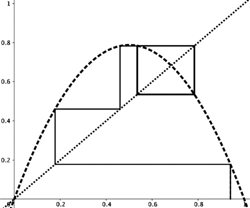
Table 2. Numerical exploration on changing r, and x₀ values for $x_{n+1}=r{x}_n(1-x_n)$, exemplifying that x_n converges to a single value $(r=2,2.58)$ or ends up cycling between two values $(r=3.00,3.15\mathrm{and}\mathrm{3.38.})$

r	x0	x1	x2	x3	x4	x5	x6	x7	x8	x9	x10
2.00	0.21	0.33	0.43	0.48	0.49	0.49	0.49	0.49	0.49	0.49	0.49
2.58	0.09	0.22	0.44	0.63	0.60	0.62	0.61	0.62	0.61	0.61	0.61
2.58	0.10	0.23	0.46	0.64	0.59	0.62	0.61	0.62	0.61	0.61	0.61
3.00	0.21	0.50	0.75	0.56	0.74	0.58	0.73	0.59	0.73	0.60	0.72
3.15	0.07	0.21	0.51	0.79	0.53	0.79	0.53	0.78	0.53	0.78	0.53
3.15	0.94	0.18	0.46	0.78	0.54	0.78	0.53	0.78	0.53	0.78	0.53
3.15	0.95	0.15	0.40	0.76	0.58	0.77	0.56	0.78	0.55	0.78	0.54
3.38	0.95	0.16	0.46	0.84	0.46	0.84	0.46	0.84	0.46	0.84	0.46
3.38	0.21	0.56	0.83	0.47	0.84	0.45	0.84	0.46	0.84	0.45	0.84

Before developing this diagram, students question how small changes in x or P can change the solutions for different r values. Using the initial value x₀, students generate successive iterations of $(x_n,f(x_n))$ which they plot using GeoGebra [13]. We generate an applet with students to represent recursion graphically by plotting $x_{n+1}$ versus x_n. The cobweb plot is created by connecting the recursive points by the vertical and horizontal segments in Figure 2, respectively, expressed as $s_{2n+1}=|(x_n,x_n)-(x_n,f(x_n))|$ and $s_{2n+2}=|(x_n,f(x_n))-(f(x_n),f(x_n))|$. When a convergent solution is found, it is observed that there is a fixed point where $x_n=f(x_n)$ or the graph will converge into a point. The case in Figure 3 demonstrates that the solution does not always converge to a single point.

Similar to the experimental approach in [3], we look into the period doubling by two-cycles, four-cycles, or more, analyzing the fixed points. For a two-cycle, x_k repeats after a certain k, such as $x_7=f^2(x_7)=x_9=x_{11}=\dots$ (see Table 2 for the case of r = 3.15). A k-cycle is observed when $x_n=f^k(x_n)$, doubling periods as k increases. As r approaches four, the logistic map in Figure 5 and periodic solution example in the Figure 4 show that pitchforked solutions are observed indicating bigger cycles.

Figure 4. Periodic Solutions for r = 3.15 and $x_0=0.94$ plotting n versus x_n.

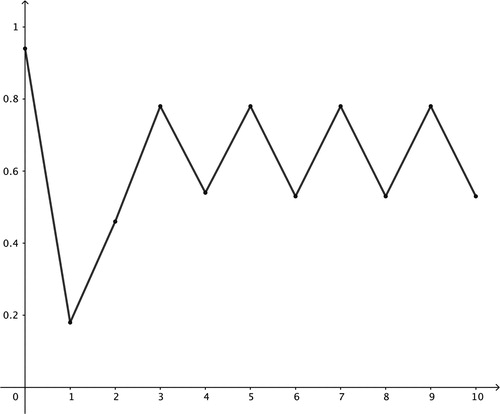
Table 2 samples and exemplifies the numerical investigation with purposeful small variations on r and x₀. It is clear that there are two steady state solutions and x converges for r = 3, r = 3.15 or r = 3.38. In addition, it is observed in Table 2 that the slightly different initial conditions $x_0=0.94$ and $x_0=0.95$, still give the same pitchforked solutions x = 0.78 and x = 0.53 after the 14th iteration.

Ultimately, sensitivity analysis shows that the recursive logistic equation is not a simple model. It demonstrates complex bifurcation behavior as depicted in the logistic map in Figure 5.

Figure 5. Logistic map and bifurcation diagram r versus x, $3<r<4$ fixed points where $x_n>x$ for $x_n=f(x_n).$

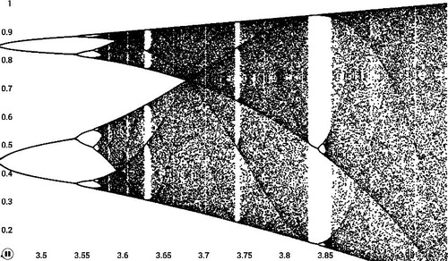
Next, we want to help students understand that this kind of chaotic behavior is not a unique phenomenon for logistic difference equations. Based on their strengths, students can be given individualized assessments to find other differential equations with unpredictable behavior, which they can explore and portray numerically and graphically. A great candidate for a follow-up is Edward Lorenz’s modeling of atmospheric convection (where he discovered chaos) using three ordinary differential equations (ODEs) [20]. This demonstrates that solutions can be highly sensitive to slight variations in the initial conditions, yielding completely divergent trajectories with an infinite set of periodic solutions. This has been used to show that, even if one knows the governing dynamical systems modeled with three ODEs, weather prediction is almost impossible.

We expect students to get informally introduced to the alternatives that they can further investigate later in their upper level classes and student research. Our goal is not to bring closure to mathematical learning as inquiry, but to leave our students curious about future pathways for growth in dealing with differential equations.

6. ASSESSMENTS

We value both the students’ mathematical models as a product and their progression through the phases of the mathematical modeling process. In particular, we value their ability to connect the differing mathematical perspectives, and to build connections among the different representations to the same modeling problem. Reflection logs and peer observations are critical to assess and support students as they go through the stages of modeling. Aligning with the goals of an inquiry-based learning environment, we emphasize communication through student writings and presentations, reflective think-alouds, and embedded assessments, so that teachers can see evidence of emerging understanding. A sample problem that we have used as a summative assessment on an exam is to solve $P\prime (t)=f(P)$, where f is a cubic function, modeling a local deer population scenario with three steady state solutions. Students were successful with this problem at the end of the semester.

Although collecting or accessing authentic data can be challenging and time-consuming, we observed that it opens doors to critical reasoning, reflection, and sense-making. As another summative assessment, we ask students to choose another locally relevant species (for example, fish, conch, sea turtles, fruit flies etc.), to come up with discrete and continuous model parameters for logistic or exponential growth curves, and, using a set of authentic local data, to evaluate how well their models perform in real life. We observe see how they interpret and formulate the relevant scenarios.

7. DISCUSSION AND CONCLUSIONS

The early phases of mathematical modeling, in particular, the problem setting phase, are very important when pursuing an interdisciplinary approach and when setting the stage for a strong emphasis on multi-representational forms. By having students simultaneously develop multiple models from both discrete and continuous perspectives, and by insisting on the use of multiple representations, students can see their solutions clearly from different contexts and develop deeper understandings.

Our teaching experiments suggest that the interdisciplinary orientation involving locally relevant problems enriches both the initial and terminal phases of the modeling process. Participants can demonstrate critical and productive engagement while setting up the problem and making informed assumptions. Furthermore, they exhibit a deeper understanding and interpretation of their solutions through a local context that they can relate to and care about. Furthermore, extensions and improvements of population models offers an opportunity for student research projects. For example, one student, who was mentored by the first author in the summer of 2017, conducted research on the spread of the Zika virus. They utilized a stochastic approach and estimated reproductive rates for local cases using data compiled from the Center for Disease Control.

Our approach helps students approach an understanding that, when modeling complex real-world scenarios, as George Box famously articulated: all models are wrong…the only question of interest is: “Is the model illuminating and useful?” [2] An enhanced treatment of the analysis of errors and the interpretation of the model, which are critical parts of the modeling process, teaches students to revisit assumptions to improve the model, so as to better reflect reality. Such modeling orientation builds a fallibilist conception of mathematics as dynamic, inquiry-driven, incomplete, and uncertain [10]. Students rarely get such opportunities in mathematics classes.

7.1. Future Revisions and Limitations

Setting up a mathematical model for a locally relevant problem, such as lionfish population dynamics, is an interdisciplinary issue that is best practiced with collaboration among faculty and community partners with relevant backgrounds and interests. This practice is not necessarily easy to achieve.

The cyclic nature of mathematical modeling requires updating the models based on new information, which allows revisiting and reinterpreting each phase, including the assumptions made before setting up the model. In our case, the lionfish population model did not take into account age or developmental stage. Building in such assumptions leads to more advanced population dynamic models. In reality, the deterministic differential equation models already involve uncertainty, due to the prediction of a reproductive ratio r. A natural extension is a stochastic logistic difference equation, where r is randomly selected from a probability distribution, within some confidence interval. Pursuing stochastic extensions of the differential and difference equations allows further connections to statistics. More joint pathways can be created between applied mathematics, statistics, and the life sciences when learning ODEs or the complimentary statistical approaches.

Slight variations on the assumptions lead to different problem formulations requiring alternative mathematical frameworks. In response to student inquiries about how to improve their model, we suggest incorporating assumptions for a discrete time delay $\tau >0$ to accommodate the time taken for egg development prior to hatching. Hutchinson’s revised logistic equation, $$\frac{dP}{dt}=rP\left(t\right)\left(1-\frac{P(t-\tau )}{K}\right),$$ where r is the intrinsic growth rate of a population, K is the environmental carrying capacity, is a viable option [19]. In this case, the shifted framework for mathematical modeling is a functional differential equation, and students will be compelled to learn more about delay differential equations [31]. Near the capacity, the solutions to delay differential equations fluctuate, unlike the flat behavior of classic logistic differential equations.

Other intra-disciplinary connections could be created by developing a population dynamics component in a statistics course. The strategy for modeling parameters such as population size (for example, mark-recapture), reproductive rates, capacity, harvesting thresholds, and abundance can be enhanced through statistical treatment.

During the modeling process, there is never one correct mathematical perspective in the Doing the Math Phase that is depicted in the GAIMME report [12]. This phase in particular can be critically improved by fostering these intra-disciplinary mathematical connections; for example, by utilizing discrete and continuous methods with differential and difference equations in the study of population dynamics.

Additional information

Funding

Part of this work was supported by National Science Foundation Grant No. 1355437. Any opinions, findings, and conclusions or recommendations expressed in this material are those of the author(s) and do not necessarily reflect the views of the National Science Foundation.

Notes on contributors

Celil Ekici

Celil Ekici currently works at the Texas A&M University - Corpus Christi as an Assistant Professor of Mathematics having served as faculty in the University of the Virgin Islands after his Ph.D. from the University of Georgia. His research interests include mathematical modeling, population dynamics, and STEM education. He enjoys pursuing locally relevant interdisciplinary mathematics learning opportunities, and integrates them into his practice with undergraduates.

Chris Plyley

Chris Plyley joined the University of the Virgin Islands in the fall of 2015 as an Assistant Professor of Mathematics, after obtaining his Ph.D. from Western University, in London, Canada. His research interests include non-associative algebra, polynomial identity theory, combinatorial number theory, and mathematics education.

REFERENCES

- Akins, J., J. Morris Jr., and S. Green. 2014. In situ tagging technique for fishes provides insight into growth and movement of invasive lionfish. Ecology and Evolution. 4(19): 3768–3777.
- Box, G. 1976. Science and statistics. Journal of the American Statistical Association. 71: 791–799.
- Brown, D. 2014. Experimental mathematics for the first year student. PRIMUS. 24(4): 281–293.
- Cornette, J. L. and R. A. Ackerman. 2011. Calculus for Life Sciences: A Modeling Approach. Washington, DC: Mathematical Association of America.
- Dance, R. and J. Sandefur. 2004. Will Your Grandchildren Have Queen Conch? http://www.uvi.edu/files/documents/College\_of\_Science\_and\_Mathematics/math\_skills/19.pdf Accessed 14 November 2017
- Desmos, Inc. 2018. Graphing calculator. https://www.desmos.com/calculator/. Accessed 15 March 2018.
- Ekici, C. and A. Gard. 2017. Inquiry based approach to transcendental functions in calculus. PRIMUS. 27: 681–692.
- Ekici, C. and C. Plyley. 2017. Inquiry based calculus with difference: Continuous and discrete modeling of mathematics in population growth. Paper presented in Joint Mathematics Meetings, Atlanta, GA.
- Ekici, C., C. Plyley, C. Alagoz-Ekici, and R. Gordon. 2018. Integrated development and assessment of mathematical and scientific modeling practices for culturally responsive STEM education. Eurasia Proceedings of Educational & Social Sciences. 9: 1–10.
- Ernest, P. 1991. The Philosophy of Mathematics Education. Routledge/Falmer.
- Freeman, S., S. L. Eddy, M. McDonough, et al. 2014. Active learning increases student performance in science, engineering, and mathematics. Proceedings of the National Academy of Sciences. 111(23): 8410–8415.
- Garfunkel, S. and M. Montgomery, (Eds). 2016. Guidelines for Assessment and Instruction in Mathematical Modeling Education (GAIMME). Philadelphia, PA: Society for Industrial and Applied Mathematics. http://www.siam.org/reports/gaimme.php. Accessed 12 March 2018.
- GeoGebra. 2018. Applet in GeoGebra. https://www.geogebra.org/m/jSEkYY5p. Accessed 16 March 2018.
- Green, S. J., J. L. Akins, A. Maljkovic, and I. M. Cote. 2012. Invasive lionfish drive atlantic coral reef fish declines. PLoS ONE. 7(3): e32596.
- Halpin, P. N., A. J. Read, E. Fujioka, et al. 2009. OBIS-SEAMAP: The world data center for marine mammal, sea bird, and sea turtle distributions. Oceanography. 22(2): 104–115.
- Hart, K. 2018. Buck Island Turtles. Data from satellite tracking and analysis tool (STAT). http://www.seaturtle.org/tracking/index.shtml/project\_id=663. Accessed 12 March 2018.
- Hirsch, C. R. and A. R. McDuffie (Eds). 2016. Mathematical Modeling and Modeling Mathematics. Reston, VA: National Council of Teachers of Mathematics.
- Hohenwarter, M., and J. Preiner. 2007. GeoGebra: Dynamic mathematics with GeoGebra. The Journal of Online Mathematics and Its Applications. 7. https://www.maa.org/external_archive/joma/Volume7/Hohenwarter/index.html. Accessed 9 December 2018.
- Hutchinson, G. E. 1948. Circular causal systems in ecology. Annals of the New York Academy of Sciences. 50: 221–246.
- Lorenz, E. N. 1963. Deterministic non periodic flow. Journal of Atmospheric Science. 20: 130–141.
- Mathematical Association of America. 2015. A Common Vision for Undergraduate Mathematical Sciences Programs in 2025. Washington DC: Mathematical Association of America. https://www.maa.org/sites/default/files/pdf/CommonVisionFinal.pdf Accessed 12 March 2018.
- May, R. 1976. Simple mathematical models with very complicated dynamics. Nature, 261: 459–467.
- Morris, J. A., K. W. Shertzer, and J. A. Rice. 2011. A stage-based matrix population model of invasive lionfish with implications for control. Biological Invasions. 13(1): 7–12.
- National Research Council. 2013. The Mathematical Sciences in 2025. Washington, DC: National Academies Press. www.nap.edu/catalog.php/record_id=15269 Accessed 16 November 2017.
- Plyley, C. and C. Ekici. 2017. Developing strategic competence with representations for growth modeling in calculus. In A. Weinberg, C. Rasmussen, J. Rabin, M. Wawro, and S. Brown (Eds), Proceedings of the 21st Annual Conference on Research in Undergraduate Mathematics Education. pp. 1102–1109. San Diego, CA.
- Petropoulou, E. N. 2010. A discrete equivalent of the logistic equation. Advances in Difference Equations. 1–15.
- Petropoulou, E. N., P. D. Siafarikas, and E. E. Tzirtzilakis. 2007. A “discretization” technique for the solution of ODEs, Journal of Mathematical Analysis and Applications. 331(1): 279–296.
- Rasmussen, C. 2001. New directions in differential equations: A framework for interpreting students’ understandings and difficulties. The Journal of Mathematical Behavior. 20(1): 55–87.
- Rasmussen, C. and O. Kwon. 2007. An inquiry oriented approach to undergraduate mathematics. Journal of Mathematical Behavior. 26: 189–194.
- Society for Industrial and Applied Mathematics. 2014. Modeling Across the Curriculum II: Report on the Second SIAM-NSF Workshop. Philadelphia, PA: Society for Industrial and Applied Mathematics. https://www.siam.org/Publications/Reports/Detail/modeling-across-the-curriculum. Accessed 9 December 2018.
- Wan, H. 2013. Modeling mosquito population dynamics: The impact of resource and temperature. Advanced Materials Research Online. 156–159: 726–731.
- Winkel, B. 2015. Modeling with differential equations in inquiry mode. https://www.simiode.org/resources/43. Accessed 10 March 2018.