Using Simulation to Teach Distributions

Abstract

Many students doubt that statistical distributions are of practical value. Simulation makes it possible for students to tackle challenging, understandable projects that illustrate how distributions can be used to answer “what-if” questions of the type often posed by analysts. Course materials that have been developed over two years of classroom trials will be shared, including (1) overviews of distributions and simulation; (2) basic capabilities of @RISK software; (3) simulation spreadsheets suitable for analysis by teams; and (4) exercises to guide the teams. These revisable materials could also be used as in-class demonstrations. Concepts illustrated include expected value, k-tiles (e.g., quartiles), empirical distributions, distribution parameters, and the law of large numbers. For those who don't have @Risk, spreadsheets are provided which demonstrate elementary risk-modeling concepts using only Excel. All materials can be downloaded from www.sba.oakland.edu/Faculty/DOANE/downloads.htm.

Supplemental data for this article can be accessed on the publisher's website.

• Computer-intensive methods
• Decisions
• Risk

1. Unanswered Questions

A few years ago, a former student (now a CFO) volunteered to talk to my introductory statistics students about how statistics helped his company. He candidly told the class that he had forgotten a lot of what he learned in statistics. But with a single example, he showed how the normal distribution had improved a management dialogue about the profit/loss implications of fluctuations in the price of a key raw material that had a strong effect on his company's bottom line. From historical data, they determined that the price variation was roughly normal, and calculated the best 5% and worst 5% cash-flow possibilities. Discussion became focused on probabilities of future cash flows. In effect, the normal distribution served as a behavioral tool to sharpen a debate.

Students were complimentary of his talk. One said that he never realized distributions were actually useful! That got me to thinking about the way I was covering distributions in my classes. Although I am a data-oriented teacher, when it came to distributions I was following the book, working problems, creating exam questions of the familiar sort, and moving on to more transparently practical topics such as confidence intervals. It was time to re-think my approach to distributions.

Most textbooks discuss distributions using formulas (for the mathematically-inclined), graphs (for the visually-oriented), and examples/scenarios/problems (for the practical-minded). The assumption is that one or more of these methods of presentation will appeal to the learner's pedagogical style. Yet doubts may trouble the thoughtful student: (1) If a measurement is only taken once, does a distribution have meaning? This question is especially germane in business and economics, where replicated experiments are rare. (2) Are distributions useful in real business decisions? I believe this second doubt arises because students see mostly sanitized or contrived textbook illustrations. (3) Students who are familiar with seemingly non-stochastic accounting statements (balance sheets, income statements, cash flow projections) may feel that financial decisions do not require statistics at all (let alone distributions).

I concluded that I needed to seek new ways to help practical-minded students (the vast majority) attempt their own answers to these questions. My search focused on the potential roles of distributions in (1) exploring our assumptions about key variables, and (2) structuring business dialogue. Basically, I was led toward a focus on risk modeling and decision-making. I wanted to capitalize on students' acceptance of computers and spreadsheets as tools of proven value in the “real world” and to encourage individual exploration. Although I am still exploring this pedagogical approach, I feel increasingly confident that it is the right direction. Although a few textbooks have begun moving this way, my personal ontogeny required me to create my own teaching materials to see what worked for the types of students I normally encounter.

The purpose of this paper is to share my ideas on using spreadsheet simulation to motivate teaching of distributions, to share classroom materials and projects that I have developed, to obtain feedback and suggestions from colleagues, and to stimulate dialogue on the simulation/decision modeling approach.

2. Existing Research

Participants in the MSMESB conferences or the annual JSM sessions on statistical education will realize that educators everywhere are using spreadsheets, collaborative projects, and case studies to help students learn statistics. It is difficult to quantify how many use simulation per se, although clearly many do, as is evident in Mills' (2002) comprehensive review of the literature on simulation in teaching statistics and probability. One suspects that many interesting approaches do not receive widespread attention. Nonetheless, there is agreement on the importance of computers (Strasser and Ozgur 1995), projects (Ledolter 1995; Love 1998; Holcomb and Ruffer 2000), cases (Parr and Smith 1998; Brady and Allen 2002), active learning (Snee 1993; Gnanadesikan 1997; Smith 1998), and cooperative learning (e.g., Magel, 1998).

Simulation materials can range from simple spreadsheets (Ageel 2002) to an entire language (Eckstein and Riedmueller 2001). Management science educators have taken an especially active role in using spreadsheet simulation of distributions to teach students to solve business problems, using both Monte Carlo simulation (e.g., Evans 2000) and process simulation (e.g., Hill 2001). While management science classes build upon and reinforce existing statistical skills for business and industrial engineering students, they do not directly address the question of how students learn statistics. Our present purpose is limited to using simulation to teach distributions, a subject which seems to have received somewhat less attention, unless we adopt broad definitions to include Central Limit Theorem demonstrations and sampling distributions.

3. Distributions as Thought Models

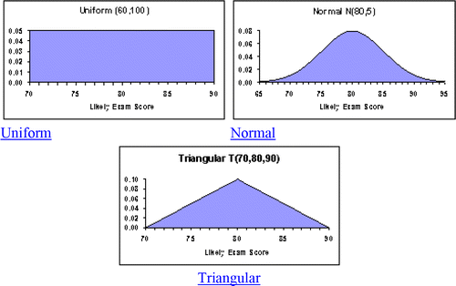
Rather than viewing distributions as descriptions of data, we can view distributions as a way of visualizing our assumptions. For example, many students will tell the instructor “I am a B student” (call it 80 on a typical grading scale). Yet grades clearly are stochastic. Any student realizes that an 80 average does not imply an 80 on every exam. A more precise statement might be, “My exam grades range from 70 to 90 but on average I get 80.” Figure 1 shows three simple ways of visualizing the situation.

Figure 1. Three Ways to Visualize Exam Scores

It can be seen that all three of the distributions shown in Figure 1 have an area of 1 (for the normal, using a triangle approximation). After seeing these diagrams, the student will deny that all scores within the range a to b would be equiprobable, hence rejecting the uniform model U(a, b). Assuming a normal distribution and the 4-sigma empirical rule (Browne 2002) we could set to model the situation as N(80, 5). 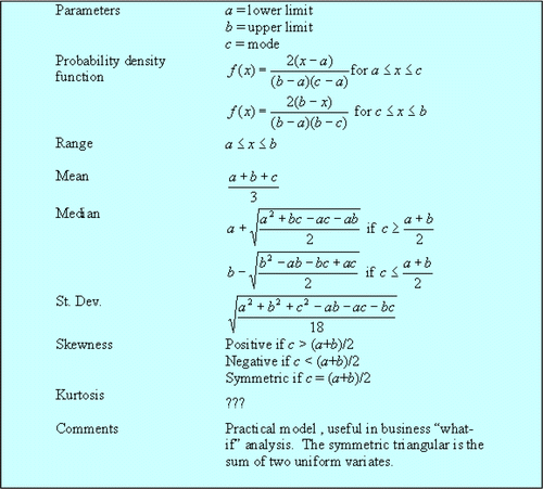Of course, students do not think in terms of normality, but upon seeing the sketch, they will agree that the implied , is a credible model of what they expect when they take an exam. But my experience suggests that the triangular distribution T(a, b, c) or T(min, max, mode) best approximates the way non-technical people think, particularly in business. Although the triangular distribution is not mentioned in most textbooks, it is attractive because (a) it is easy to visualize, (b) it is flexible, (c) it prevents extremes, (d) it can be skewed, and (e) areas can be found using the familiar formula A = ½bh. The symmetric triangular resembles a normal, except that it lacks extreme values (see Appendix A for a few basic facts about the triangular distribution).

4. Simulation Models

Monte Carlo simulation variables can be either deterministic (non-random or fixed) or stochastic (random variables). If a variable is stochastic, we must hypothesize its distribution (normal, triangular, etc.). By allowing the stochastic variables to vary, we can study the behavior of the output variables that interest us, to establish their ranges and likelihood of occurrence. But we are mainly interested in the sensitivity of our output variables to variation in the stochastic input variables.

Table 1. Components of a Simulation Model

Component	Explanation
List of deterministic factors F1, F2, …, Fm	These are quantities that are known or fixed, or whose behavior we choose not to model (i.e., exogenous).
List of stochastic input variables V1, V2, …, Vk	These are quantities whose value cannot be known with certainty, and are assumed to vary randomly.
List of output variables O1, O2, …, Op	These are stochastic quantities that are important to a decision problem, but whose value depends on many things in the model and whose distribution is not easily found.
Assumed distribution for each stochastic input variable	These are chosen from known statistical distributions, such as normal, Poisson, triangular, and so on.
A model which specifies the rules or formulas that define the relationships among Fs and Vs	Formulas including simple accounting identities such as Profit = Revenue – Cost or End Balance = Begin Balance – Withdrawals+ Deposits, or behavioral hypotheses such as Car Sales = b0 + b1(Personal Income After Taxes) + b2(Net Worth) + b3(3-month T-Bill Interest Rate).
A simulation method that produces random data from the specified distributions and captures the results.	This is a programming language (such as VBA) although it may be embedded invisibly in a spreadsheet with built-in functions like Excel's RAND() or other add-ins.
An interface that summarizes the model's inputs, outputs, and simulation results.	Typically, spreadsheet tables or graphs to summarize the outcomes of the simulation.

5. Classroom Demonstration

Before assigning any independent projects, the teacher needs a simple classroom demonstration. This one uses a simple spreadsheet which can be downloaded along with the student projects. The Axolotl Corporation sells three products (A, B, and C). Prices are set competitively, and are assumed constant. The quantity demanded, however, varies widely from month to month. To prepare a revenue forecast, the firm sets up a simple simulation model of its input variables, as shown in Table 2. The output variable of interest is total revenue P_A Q_A + P_B Q_B + P_C Q_C.

Table 2. Simulation Setup for Revenue Calculation

Variable	Type	Product A	Product B	Product C
Price	Deterministic	PA = 80	PA = 150	PA = 400
Quantity	Stochastic input	Normal QA ∼N(50, 10)m =50,s = 10	TriangularQB ∼T(0, 40, 5) Min =0, Max = 40, Mode = 5	Exponential QC ∼E(2.5) l = 2.5
Revenue	Stochasticoutput	PA QA	PB QB	PC QC

Variation in the quantity demanded would make it difficult to predict total revenue. We could predict its mean, based on the mean of each distribution, but what about its range? This demonstration shows that simulation reveals things that are not obvious.

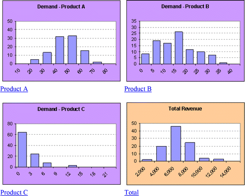
Table 3 shows the results of a typical simulation run using 100 Monte Carlo iterations (i.e., each input cell value is sampled, results are computed, and the process is repeated 100 times). This simulation can be repeated another 100 times by clicking a button. Results will vary, but as long as the number of iterations is reasonably large, the conclusions will be similar.

Table 3. Results of 100 Iterations of Revenue Simulation

Percentile	Product A	Product B	Product C	Total Revenue
Min	26	1	0	4,180
5%	34	4	0	4,745
25%	44	8	1	5,943
50%	50	14	2	7,000
75%	56	20	3	8,340
95%	64	32	6	10,022
Max	69	35	11	10,780
Sample Mean	49.85	15.11	2.30	7,335
Theory Mean	50	15	2.5	7,250

Notem_B = (a + b + c)/3 = (0 + 40 + 5)/3 = 15.m_A = 50 and m_C = 2.5 we can find the theoretical mean of total revenue as P_A m_A + P_B m_B + P_C m_C = (80)(50) + (150)(15) + (400)(2.5) = 4,000 + 2,250 + 1,000 = 7,250. This compares well with the sample result over 100 iterations. Although product A contributes the most to total revenue at the mean, this may not be the case in a particular simulation, because demand can fluctuate.

These results suggest that Axolotl's revenue could be as low as $4,180 or as high as $10,780, with a 50% chance (25th and 75th percentiles) of revenue between $5,943 and $8,340. Median revenue seems to be below the mean, suggesting that total revenue is right-skewed. That is e expected, since both the triangular (Product B) and exponential (Product C) are right-skewed distributions (as is also evident in the simulation results for demand for Products B and C). The symmetric normal distribution (Product A) is reflected in the simulation results, which lie well within the limits. Figure 2 summarizes the simulation results visually. Notice that color-coding is used in the spreadsheet and graphs to distinguish inputs (purple) from outputs (orange).

Figure 2. Histograms for 100 Iterations of Revenue Simulation

6. Student Simulation Projects

Once the basic idea is in place, it is natural to have students explore what can happen when they use distributions for stochastic decision parameters in a new scenario. My design goals were to develop scenarios that (1) were entertaining, (2) involved familiar problems, (3) had a clear “bottom line,” (4) called for “what-if” analysis, and (5) were complex enough that the solutions weren't obvious. In short, I set out to create “light” simulation scenarios with sufficient relevance to attract practical-minded students.

Initially, I selected @Risk as the simulation tool (although Crystal Ball would be equivalent) because I was able to negotiate a reasonable one-year academic site license fee (about $500). My university's Teaching and Learning Committee underwrote the first year's cost, and my academic unit agreed to pick up the license thereafter if the experiment proved successful. I developed three scenarios using @Risk and tried them in the classroom. Realizing that there is a learning curve for @Risk (as well as an added cost) I later developed Excel-only versions, although at the sacrifice of some powerful features of @Risk.

The scenarios presented here are intended to be undertaken by student teams of two students in a one-hour computer lab session under instructor supervision. I find that more than two students cannot effectively share a single computer and have trouble agreeing on the joint report under a tight deadline. Why use teams at all? First, because even if one partner is dominant, interaction is beneficial to both. Second, teams more closely approximate the workplace. Each in-class project can be done in 60-90 minutes if the simulation tools are demonstrated during a prior lecture and scenario overviews and project instructions are handed out in advance. The one-hour deadline forces closure, just as in the “real world” where a report must be done by the deadline even if a better one could be written. A little time pressure rewards teams who do not dawdle.

The three scenarios discussed here use only the normal , and triangular T(a,b,c) distributions because they are flexible yet easy to understand. Each scenario involves a problem faced by a hypothetical character named “Bob.”

• Scenario 1: Bob's Stochastic Balance Sheet (to illustrate that net worth is stochastic in the sense that it depends on the uncertain market value of assets and that some asset values are more predictable than others and may have different distributions)

• Scenario 2: Bob's Mail Order Business (to illustrate that a breakeven analysis is stochastic in that it depends on random variables not under the control of the business, and that key parameters may have different distributions)

• Scenario 3: Bob's Statistics Grades (to illustrate that grades are stochastic in the sense that there is variation in performance on exams, quizzes, projects, and lab work, and that the means and variances may differ on different tasks)

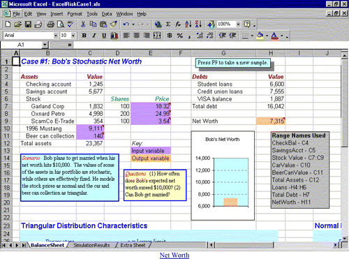
We illustrate with Bob's Stochastic Balance Sheet. The basic spreadsheet (Excel version) is shown in Figure 3. Where relevant, cell range names are used (e.g., Net Worth) to increase students' familiarity with this useful alternative to cell references (e.g., H9). Comments have been added to cells that specify stochastic inputs (purple highlight) or stochastic outputs (orange highlight). The idea is that the output cells are “bottom line” variable of interest while input cells are the “drivers” of the output(s).

Figure 3. Bob's Stochastic Balance Sheet

The spreadsheet contains a description of the scenario, a set of questions, and a graph showing Bob's net worth. The idea is that on a given day, Bob's actual net worth depends on the market value of his assets. Some of his asset and liability values are deterministic (e.g., checking account, savings account, student loans) while the values of his car, beer can collection, and stocks (and hence his net worth) are stochastic. Table 4 shows the characteristics of the stochastic inputs (distribution, skewness, coefficient of variation).

Table 4. Distributions Used in Bob's Stochastic Balance Sheet

Asset	Distribution	Comments
Mustang	T(8000,15000,10000)	Right-skewed
Beer can collection	T(0,1000,50)	Very right-skewed
Garland stock	N(15.38,3.15)	Symmetric, large C.V.
Oxnard stock	N(26.87,2.02)	Symmetric, small C.V.
Scamco stock	N(3.56,0.26)	Symmetric, small C.V.

The graph and highlighted cells will update with new simulated values each time F9 is pressed. The goal is to get the learner to visualize (1) what values could appear in each cell, and (2) what these distributions say about Bob's reasoning. For example, Bob thinks that if he finds the right buyer, his Mustang could be worth up to $15,000. He is quite sure he won't get less than $8,000. He figures that $10,000 is the most likely value. This way of thinking strikes many students as congruent with their own.

While the prices of Bob's stocks vary without limits, as a practical matter even is conservative. Following the logic of probability plots (D'Agostino and Stephens 1986), the range that is likely to be observed in a sample is from F⁻¹(0.5/n) to F⁻¹(1-(0.5/n)) where F⁻¹ is the inverse of the cumulative distribution function. For n = 100, the likely sample extremes are from F⁻¹(0.005) to F⁻¹(0.995). For the Garland stock this implies values between 15.38 ± 2.576(3.15) or $7.27 to $23.91. @Risk offers a truncated normal, to prevent extreme values, but its theoretical properties are awkward.

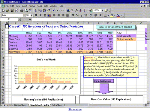
In this Excel-only version of Bob's Stochastic Balance Sheet, a second worksheet shows the results of 100 iterations of sampling. This provides a basis for answering the question posed (and suggests some new questions). There are histograms for each input and output variable. Every time F9 is pressed, 100 new iterations will occur. Students can observe that despite variation in the individual stochastic cells, there is stability in the mean, standard deviation, and k-tiles of each stochastic variable.

Figure 4. Simulation Summary for Bob's Balance Sheet (Excel Version)

7. Using @Risk for Simulation

@Risk is an Excel add-in software package with powerful simulation capabilities (see Winston 2001). The general idea of @Risk is to provide built-in functions to create random values in designated cells. When we paste an @Risk input function for the desired statistical distribution in a cell, its contents become stochastic, so that every time the spreadsheet is updated a new value will appear. For example, an input cell containing =RiskNormal(26,4) is a random variable with and . All the common distributions are available from Excel's Insert|Function menu. An output cell is calculated as usual except that =RiskOutput()+ is added in front of the cell's contents (e.g., =RiskOutput + TotalAssets – TotalDebt where TotalAssets and TotalDebt are defined elsewhere in the spreadsheet (of course, you can also use cell references like C12 and H7 instead of cell names). Thus, @Risk automates tasks that otherwise would require VBA programming.

Each time F9 is pressed, the spreadsheet will show updated values of all input and output cells. In replication mode, we can do up to 10,000 replications while @Risk keeps track of all simulated values of the input and output cells. For those variables, empirical distributions can be displayed in tables (statistics, percentiles) or charts (histograms, cumulative distributions). Using sliders, you can reveal any desired percentile on the cumulative distribution. Tornado charts can be used to reveal sensitivities of output variables to all the input variables.

Figure 5. Buttons to Set Up the Simulation

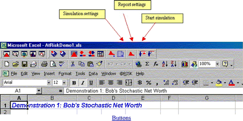
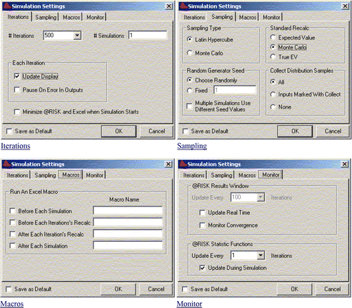
The @Risk toolbar lies above the regular Excel toolbar, as illustrated in Figure 5. The @Risk setup screens and typical settings are shown in Figure 6. Experience suggests that 500 iterations will suffice for the distributions used in our scenarios.

Figure 6. Suggested Simulation Settings

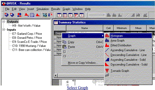
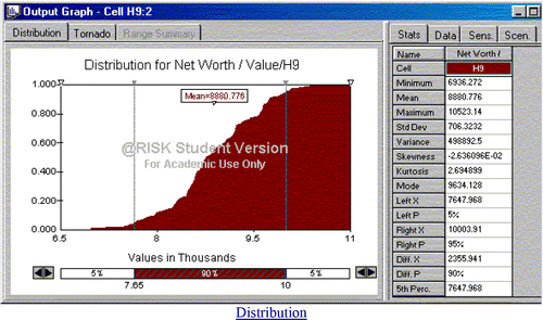
Various reports can be generated and placed either in a new workbook or in the active workbook. To begin, click the Start Simulation button. A screen like Figure 7 will appear. Select a variable by clicking its row tab (in this illustration, we chose Output H9-Net Worth). You will get a menu of graphs that are available.

Figure 7. Selecting a Graph

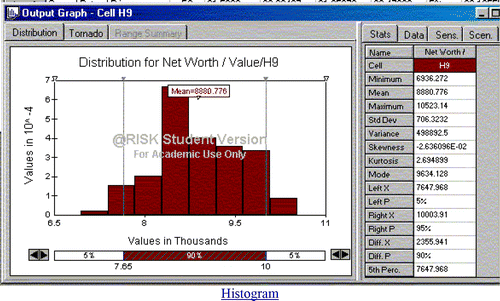
By default, the middle 90% of the outcomes are shown. In Figure 8, the distribution of net worth is symmetric and platykurtic with a mean of $8,881, exceeding $10,000 only about 5% of the time.

Figure 8. Histogram of 500 Iterations of Net Worth

You can drag the vertical sliders to show different percentiles. This is easy, but inexact. To select integer percentiles, use the arrows at the bottom of the histogram. Switching to an ascending cumulative distribution (Figure 9) we see essentially the same thing, though the tails show somewhat more detail.

Figure 9. Distribution of Net Worth for 500 Iterations

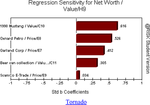
For sensitivity analysis, click on the Tornado tab to see a list of factors that explain variation in net worth, listed in order of importance, as illustrated in Figure 10. Bars that face right are positively affecting the output variable, while bars (if any) that face left are affecting the output variable negatively. Sensitivities can range from −1.0 to +1.0, with values near zero indicating lack of importance. Here, the Mustang value and Oxnard and Garland stock prices are the most important input variables, while beer cans are less important and the ScamCo stock contributes little variation to net worth.

Figure 10. Tornado Graph for Sensitivity Analysis

8. Issues and Discussion

After using these materials three times in a required undergraduate class and once in an MBA class, I can report that students are attracted to this approach. One of the exercises asks the team to rate advantages and disadvantages of @Risk simulation. Based on their comments and my own observations, I conclude that the advantages of @Risk are its ease of use, power, and versatility. Drawbacks of @Risk are its high price, lack of general availability to students after they leave the university, and rarity of use in universities, partly due to administrative and licensing issues. These drawbacks have prompted some educators to develop their own Excel-only simulation add-ins (e.g., Eckstein and Riedmueller 2001), although they must still teach students to use the add-in.

These are the motivations for my simple Excel-only versions of the simulation spreadsheets without add-ins, despite the loss of powerful features such as sensitivity analysis and slider bars for percentiles. Another limitation is that the Excel-only histograms are set up for the initial parameter values, so they will not look right if the parameters are changed. But an advantage of the Excel-based versions is that curious students can “see how it is done” by looking at the cells, histogram bins, and tables of results, whereas @Risk's functions are “black boxes.” Without VBA programming, we can create the normal and triangular distributions used in the three scenarios, although at the cost of some unaesthetic columns of intermediate calculations. While VBA would be needed to create most discrete distributions (e.g., binomial, Poisson) Appendix B shows Excel functions to create random data from a few common distributions.

Another issue is that mainstream textbooks do not discuss risk modeling, @Risk, or simulation in general. These become extra topics which impose a burden on the instructor. Students are usually suspicious of material that is “not in the book,” fearing that their instructor is going to subject them to some kind of iconoclastic experiment. There now are textbooks on risk modeling (e.g., Albright, Winston, and Zappe 1999; Evans and Olsen 2001; Moore and Weatherford 2001). But mainstream practice evolves very slowly. It is noteworthy that some popular textbook authors have tried abolishing some distribution tables (e.g., binomial, Poisson), partly for brevity but also because Excel functions make tables obsolete. But can students take exams without tables?

Syllabus crowding is also an issue. With an already-crowded syllabus, it is not easy to convince faculty to spend 2-3 extra class days for risk modeling and lab projects. My colleagues have not jumped on the @Risk bandwagon for this explicit reason. There is also resistance to teaching yet another software package like @Risk. We already have our hands full with Excel and Minitab.

Should we reduce traditional treatment of distributions to yield curricular space for simulation and risk modeling? Can simulation and risk modeling cases somehow increase understanding enough to replace time currently spent on distributions? The answer may be “not at this point.” Perhaps if Excel had built-in simulation capabilities the answer could be “yes.” Faculty may become convinced if they see that students enjoy doing risk modeling projects and gain useful knowledge. Experts (e.g., Love and Hildebrand 2002) do recommend less lecture and more use of collaborative cases, so there is support for experimentation of this sort.

One contemporary thought question: would companies whose defined benefit pension funds in 2002 faced under-funding because stock market returns have been subnormal have found it useful to engage in @Risk simulation, using (say) triangular distributions of possible returns on their investment portfolios? If so, perhaps at least a contingency plan could have been created to anticipate cash flow problems.

9. Downloadable files

Interested parties can download the 542K file JSE.zip directly or from my web site:

www.sba.oakland.edu/Faculty/DOANE/downloads.htm

Appendix C lists the files contained in JSE.zip. The Word files and @Risk scenarios can be modified to fit local situations. However, as explained earlier, care must be taken in modifying the Excel-only versions because of assigned variable names, fixed histogram scales, and complex cell links. Permission is given to use these materials in an academic setting, as long as they are not resold for profit and are properly attributed. As a courtesy, I would appreciate comments and suggestions from those who use them.

Attention users of Excel 2003

Microsoft has released a March 23, 2004 update to Microsoft Office Excel 2003 to fix a problem in Excel 2003 that can cause the RAND(), RANDBETWEEN(), SLOPE(), INTERCEPT(), FORECAST(), and STEYX() functions to return values that are incorrect. This problem could affect some of the spreadsheets mentioned in this article. To download the Excel 2003 update, go to http://www.microsoft.com/downloads/details.aspx?familyid=DD344A47-1FAF-4DB6-94CD-4FEC532AC044&displaylang=en

Appendix A

Characteristics of the Triangular Distribution

Appendix B

Random Numbers in Excel

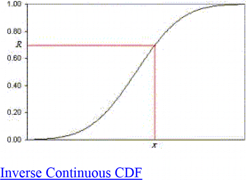
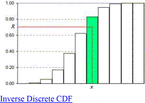
Random numbers are at the heart of any simulation. In general, if you know F(x), the cumulative distribution function (CDF) of your distribution, you generate a uniform U(0,1) random number R and then find F⁻¹(R) where F⁻¹ is the inverse of the CDF. Essentially, what you have to do is to set F(x)=R and then solve for x, as illustrated in Figure 11. However, this is sometimes easier said than done, because finding may be tricky, especially for discrete distributions as in Figure 12. With VBA it is not difficult, and there are plenty of commercial packages that do it. But it is harder if you are a do-it-yourself person who wants only to use the functions available within Excel. Table 13 shows Excel functions to create random data for a few common distributions.

Figure 11. Inverse Continuous CDF

Figure 12. Inverse Discrete CDF

Table 5. Creating Random Data in Excel

Distribution	What to Put in Excel Cell	Explanation
Uniform U(0, 1)	=RAND()	Built-in Excel function
Uniform U(a, b)	=$A$1+($A$2-$A$1)*RAND()	$A$1 is the minimum and $A$2 is the maximum (or use cell names like Xmin and Xmax).
Normal N(0, 1)	Method A: =NORMSINV(RAND()) Method B: =SQRT(−LN(RAND()))*COS(2*PI()*RAND())	Excel's inverse normal function or do-it-yourself Box-Muller transform.
Normal (m, s)	Method A: =NORMINV(RAND(),$A$1,$A$2) Method B: =$A$1+$A$2*SQRT(−2*LN(RAND()))*COS(2*PI()*RAND())	$A$1 is the mean and $A$2 is the standard deviation (or use cell names like Mu and Sigma).
Exponential E(l)	=-LN(RAND())*$A$1	$A$1 is the mean Poisson arrival rate (or use cell name like Lambda)
Triangular T(a, b, c)	No single cell formula but can be done in Excel with two cells.	Better to use @Risk or Crystal Ball.
Bernoulli B(p)	=IF(RAND()<$A$1,1,0)	$A$1 is the probability of success (or use a cell name like ProbSuccess)

Appendix C

Downloadable Files

www.sba.oakland.edu/Faculty/DOANE/downloads.htm

Table

File Name	Type	Contents
SimulationBasics.doc	Word	Brief handout on simulation and distributions (examples, functions, Excel, @Risk)
[e-mail]	Word	Optional handout on @Risk software (methods, iterations, output options) to get teams started if they use the @Risk versions of the cases.
ProjectInstructions.doc	Word	Instructions to student teams for in-class projects using the case studies. Includes separate instructions for Excel-only and @Risk versions.
ThreeProductExample.xls	Excel	Suggested in-class demonstration using only Excel. Illustrates normal, triangular, and exponential distributions using a familiar business example.
@RiskVersion-Case1.xls @RiskVersion-Case2.xls @RiskVersion-Case3.xls	Excel	Three Excel spreadsheet cases using @Risk functions, with questions to be answered by student teams. Requires @Risk software. Stochastic cells will show #NAME? until the @Risk Add-In is installed and @Risk is started.
ExcelVersion -Case1.xls ExcelVersion-Case2.xls ExcelVersion-Case3.xls	Excel	Three Excel spreadsheet cases containing formulas, questions to be answered by the student teams, and a simulation results worksheet. Initial stochastic cell values change when F9 is pressed. Fewer capabilities than the @Risk version, but works using only Excel without any add-ins.