Identifying Heterogeneity in Dynamic Panel Models with Individual Parameter Contribution Regression

Abstract

Dynamic panel models are a popular approach to study interrelationships between repeatedly measured variables. Often, dynamic panel models are specified and estimated within a structural equation modeling (SEM) framework. An endemic problem threatening the validity of such models is unmodelled heterogeneity. Recently, individual parameter contribution (IPC) regression was proposed as a flexible method to study heterogeneity in SEM parameters as a function of observed covariates. In the present paper, we derive how IPCs can be calculated for general maximum likelihood estimates and evaluate the performance of IPC regression to estimate group differences in dynamic panel models in discrete and continuous time. We show that IPC regression can be slightly biased in samples with large group differences and present a bias correction procedure. IPC regression showed generally promising results for discrete time models. However, due to highly nonlinear parameter constraints, caution is indicated when applying IPC regression to continuous time models.

Keywords:

• Autoregressive cross-lagged model
• continuous time modeling
• heterogeneity
• structural equation modeling

Introduction

Dynamic panel models (Hsiao, 2014) are routinely used in econometrics, psychology, and sociology to model the coupling between several repeatedly measured variables. Building upon the idea of Granger causality (Granger, 1969), dynamic models allow answering questions concerned with the direction and strength of reciprocal relationships. Especially in psychological research, it is common practice to specify and estimate dynamic panel models within the structural equation modeling (SEM) framework (e.g., Allison, Williams, & Moral-Benito, 2017; Bollen & Brand, 2010; Zyphur, Allison et al., 2019, Zyphur, Voelkle et al., 2019).

An endemic problem that complicates the analysis of longitudinal panel data are systematic differences across individuals or groups. For instance, individuals may show stable, trait-like differences in the mean levels; a random shock might have a long-lasting effect on some persons, while its effect vanishes quickly for others; or the coupling between processes may differ across subjects. By overlooking such heterogeneity, researchers risk drawing incorrect conclusions from their data (Halaby, 2004).

Heterogeneity can often be explained through covariates such as demographic variables, biomarkers, or personality traits. Various approaches have been suggested to identify if and how covariates are linked to individual or group differences in dynamic panel models. A popular way is the use of multilevel models with random effects (e.g., Singer & Willet, 2003). For instance, dynamic panel models are often specified with random intercepts to account for trait-like differences in the mean level of the observed variables (e.g., Hamaker, Kuiper, & Grasman, 2015). By regressing random effects on covariates, multilevel models can also be used to explore correlates and predictors of heterogeneity. Another popular approach to investigate heterogeneity are multi-group structural equation models (MGSEM; Sörbom, 1974) which allow the specification of panel models with different parameter values across groups. MGSEMs are particularly useful if the number of groups is small. However, using MGSEMs to disentangle the effects of many grouping variables can become tedious as multiple MGSEMs need to be specified and estimated. Fortunately, there exist approaches to perform such testing automatically, which become feasible with large sample sizes: Brandmaier, von Oertzen, McArdle, and Lindenberger (2013) and Brandmaier, Prindle, McArdle, and Lindenberger (2016) proposed a combination of MGSEMs and recursive partitioning methods to recover groups with similar parameter values. These so-called SEM trees or SEM forests fit a large number of MGSEMs to identify which grouping variables are important. Recently, Brandmaier, Driver, and Voelkle (2018) also applied these methods to dynamic panel models.

While the above methods are able to detect heterogeneity in a wide range of situations, they also come with certain drawbacks. The use of random effects to detect individual or group differences in dynamic panel models is often hindered by difficulties to specify the random effects for certain types of parameters. Whereas including random effects for intercept parameters is relatively straightforward, specifying random effects for regression and variance parameters is much more problematic and usually requires Bayesian methods (e.g., Driver & Voelkle, 2018; Schuurman, Ferrer, de Boer-Sonnenschein, & Hamaker, 2016). A drawback of MGSEM and MGSEM-based approaches like SEM trees and forests is that these methods require either categorical grouping variables or require continuous covariates to be split into meaningful grouping variables which might obscure the relationship between differences in a parameter and a continuous covariate. Furthermore, SEM trees and forests may experience difficulties when there is a clear set of target parameters of interest. Since these methods compare the group-wise likelihood, which considers differences in all parameters across all levels of the covariates jointly, the difference of interest may be masked if a larger difference is found in other parameters. This masking effect is well-known in the regression mixture literature (George et al., 2013) and may occur particularly in the case of distributional misspecification (e.g., Usami, Hayes, & McArdle, 2017). Finally, especially in large data sets, the computational burden of methods like Bayesian multilevel models, SEM trees, and SEM forests often constitutes a major impediment to implement these approaches in practice.

As an alternative approach to identify and estimate heterogeneity in dynamic panel models, we propose the use of individual parameter contribution (IPC) regression (Oberski, 2013). As we will discuss in the following, the IPC regression framework allows modeling SEM parameters as a function of covariates. Put shortly, IPC regression proceeds in three steps. First, a theory-driven (confirmatory) SEM is specified and estimated. Second, individual contributions to all model parameters are calculated using the case-wise derivative of the log-likelihood function. The resulting IPCs approximate individual-specific parameter values. Third, the IPCs are regressed on a set of categorical or continuous covariates to explain group differences or individual differences in the parameters. For instance, a researcher could regress the IPCs to one parameter on individuals’ age to test whether this parameter is invariant to age differences or to estimate how the parameter changes as a function of age.

The primary advantages of IPC regression over other approaches to heterogeneity outlined above are its simplicity, flexibility, and low computational demand. IPC regression separates the estimation of the theory-driven model from the investigation of individual group differences. This separation is especially useful if the theory-driven model is complex, that is, has many observed variables and parameters. Although the underlying mathematics can be challenging, on the side of the applied researcher, basic knowledge of linear regression analysis is sufficient for successfully applying IPC regression in practice. IPC regression allows testing every type of SEM parameter (e.g., means, variances, covariances) for individual or group differences without the need for specifying random effects. Moreover, the method allows studying the effect of multiple grouping variables as well as continuous covariates and their interactions. Furthermore, IPC regression is a computationally lightweight procedure that can be performed in seconds.

IPCs are not limited to SEMs and can be derived for every type of maximum likelihood estimate. The contributions are calculated by linearizing the case-wise derivative of the log-likelihood function around the maximum likelihood estimates. The case-wise derivative of the log-likelihood function, also known as score function, has long been used to investigate the plausibility of statistical models (e.g., Zeileis, 2005; Zeileis & Hornik, 2007). Recently, score-based tests became popular in the exploration of measurement invariance in SEM (Merkle, Fan, & Zeileis, 2014; Merkle & Zeileis, 2013; Wang, Merkle, & Zeileis, 2014; Wang, Strobl, Zeileis, & Merkle, 2018). These score-based tests are used to test measurement invariance with respect to a continuous or ordinal auxiliary variable. IPC regression is different to these tests by providing estimates of how a model parameter varies as a function of covariates. Other frequently applied score-based approaches to identify misspecification in SEMs are the modification index (Sörbom, 1989) and the expected parameter change (Saris, Satorra, & Sörbom, 1987), which both test the validity of certain parameter restrictions but do not address the problem of parameter heterogeneity even though they are closely related (Oberski, 2013).

As of now, IPC regression has only been evaluated for a confirmatory factor analysis model (CFA; Brown, 2006). In a Monte Carlo simulation, Oberski (2013) reported excellent finite sample performance. We will later show that these results do not fully generalize to more complex models such as dynamic panel models. In general, large individual or group differences in one specific parameter can lead to biased IPC regression estimates for that specific parameter and also may lead to biased IPC regression estimates for other parameters. As a consequence, large differences in one parameter can increase the risk of a type I error in other constant parameters. To solve this problem, we propose a bias correction procedure termed iterated IPC regression that we recommend for dynamic panel models. The remainder of this article is organized as follows: first, we will briefly present bivariate dynamic panel models in discrete and continuous time. Second, IPC regression is formally introduced. Third, we evaluate the finite-sample properties of IPC regression for dynamic panel models in two simulation studies.

Autoregressive and cross-lagged models for panel data

The following section gives an outline of the SEM specifications for two simple dynamic panel models in discrete and continuous time that will be used throughout the present article. Readers unfamiliar with dynamic panel models are referred to Biesanz (2012). More details about the continuous-time models are given by Voelkle, Oud, Davidov, and Schmidt (2012).

Figure 1 shows a path diagram for a bivariate dynamic panel model for three waves of data. This structural model can be described with the following two equations:

(1) $x_{i,t}={\beta }_{xx}{x}_{i,t-1}+{\beta }_{xy}{y}_{i,t-1}+u_{i,t}$(1)

(2) $y_{i,t}={\beta }_{yy}{y}_{i,t-1}+{\beta }_{yx}{x}_{i,t-1}+v_{i,t},i=1,\dots ,n,t=2,3$(2)

FIGURE 1 Path diagram of a bivariate autoregressive and cross-lagged panel model for three waves of data.

Here, $x_{i,t}$ and $y_{i,t}$ are the measurements of two different variables of individual $i$ at time point $t$. For sake of simplicity, we assume that $x$ and $y$ are free of measurement error and mean centered.

The regression coefficients ${\beta }_{xx}$ and ${\beta }_{yy}$ are called autoregressive parameters and they describe the stability in each $x$ and $y$ from one measurement occasion to the next. The regression coefficients ${\beta }_{xy}$ and ${\beta }_{yx}$ are referred to as cross-lagged effects and indicate how $x$ influences $y$ and vice versa. The initial assessments of $x$ and $y$ are treated as exogenous variables with zero mean and variance ${\varphi }_{xx}$, ${\varphi }_{yy}$ respectively, and covariance ${\varphi }_{yx}$. For the remaining measurement occasions, $u$ and $v$ denote the dynamic error terms. The variance and covariance parameters of the dynamic error terms are symbolized by ${\psi }_{xx}$, ${\psi }_{yy}$, and ${\psi }_{yx}$ respectively.

Equations (3a(3a) ${\mathbf{y}}_i=\mathbf{B}{\mathbf{y}}_i+{\zeta }_i$(3a) )–(3c(3c) $\mathrm{C}\mathrm{o}\mathrm{v}({\zeta }_i,{\zeta }_i)=\mathbf{\Phi }=\left[\begin{array}{cccccc}{\varphi }_{xx}& {\varphi }_{yx}& 0& 0& 0& 0\\ {\varphi }_{yx}& {\varphi }_{yy}& 0& 0& 0& 0\\ 0& 0& {\psi }_{xx}& {\psi }_{yx}& 0& 0\\ 0& 0& {\psi }_{yx}& {\psi }_{yy}& 0& 0\\ 0& 0& 0& 0& {\psi }_{xx}& {\psi }_{yx}\\ 0& 0& 0& 0& {\psi }_{yx}& {\psi }_{yy}\end{array}\right]$(3c) ) show the SEM specification of the model in Figure 1:

(3a) ${\mathbf{y}}_i=\mathbf{B}{\mathbf{y}}_i+{\zeta }_i$(3a)

(3b) $\left[\begin{array}{c}{x}_{i,1}\\ y_{i,1}\\ x_{i,2}\\ y_{i,2}\\ x_{i,3}\\ y_{i,3}\end{array}\right]=\left[\begin{array}{cccccc}0& 0& 0& 0& 0& 0\\ 0& 0& 0& 0& 0& 0\\ {\beta }_{xx}& {\beta }_{xy}& 0& 0& 0& 0\\ {\beta }_{yx}& {\beta }_{yy}& 0& 0& 0& 0\\ 0& 0& {\beta }_{xx}& {\beta }_{xy}& 0& 0\\ 0& 0& {\beta }_{yx}& {\beta }_{yx}& 0& 0\end{array}\right]\left[\begin{array}{c}{x}_{i,1}\\ y_{i,1}\\ x_{i,2}\\ y_{i,2}\\ x_{i,3}\\ y_{i,3}\end{array}\right]+\left[\begin{array}{c}{x}_{i,1}\\ y_{i,1}\\ u_{i,2}\\ v_{i,2}\\ u_{i,3}\\ v_{i,3}\end{array}\right]$(3b)

(3c) $\mathrm{C}\mathrm{o}\mathrm{v}({\zeta }_i,{\zeta }_i)=\mathbf{\Phi }=\left[\begin{array}{cccccc}{\varphi }_{xx}& {\varphi }_{yx}& 0& 0& 0& 0\\ {\varphi }_{yx}& {\varphi }_{yy}& 0& 0& 0& 0\\ 0& 0& {\psi }_{xx}& {\psi }_{yx}& 0& 0\\ 0& 0& {\psi }_{yx}& {\psi }_{yy}& 0& 0\\ 0& 0& 0& 0& {\psi }_{xx}& {\psi }_{yx}\\ 0& 0& 0& 0& {\psi }_{yx}& {\psi }_{yy}\end{array}\right]$(3c)

The resulting model-implied covariance matrix of $x$ and $y$ is given by

(4) $\mathrm{C}\mathrm{o}\mathrm{v}({\mathbf{y}}_i,{\mathbf{y}}_i)=\mathbf{\Sigma }(\theta )={\left({\mathbf{I}}_6-\mathbf{B}\right)}^{-1}\mathbf{\Phi }{\left[{\left({\mathbf{I}}_6-\mathbf{B}\right)}^{-1}\right]}^{\mathrm{T}},$(4)

where $\theta$ is a vector with the model parameters and ${\mathbf{I}}_6$ denotes an identity matrix of order six.

Although not explicitly stated, the temporally spacing between assessments plays an important role in the model as presented in Figure 1. The model treats time as a discrete variable that indicates the temporally ordering of the assessments and is therefore also referred to as discrete-time dynamic panel model. As pointed out elsewhere (e.g., Oud, 2007; Oud & Delsing, 2010; Voelkle et al., 2012), treating time as a discrete variable complicates comparing estimates from models with different sample schemes and can bias estimates if assessments are not equally spaced. A solution to these problems is treating time as a continuous variable using stochastic differential equation models (Oud & Jansen, 2000; for a recent overview of continuous-time modeling in the behavioral and related sciences, see van Montfort, Oud, & Voelkle, 2018). These continuous-time dynamic panel models allow estimating continuous-time parameters which can be used to extrapolate to any arbitrary time point.

Following Voelkle et al. (2012), we specify a continuous-time model by constraining the discrete-time model parameters from Figure 1 to functions of underlying continuous-time parameters $\mathbf{A}$ and $\mathbf{Q}$, and the time intervals $\mathrm{\Delta }{t}_j$. The new parameter matrix $\mathbf{A}$ corresponds to the continuous-time version of auto- and cross-lagged effects, the drift parameters, while $\mathbf{Q}$ contains the continuous-time version of dynamic error term variance parameters, or diffusion parameters:

(5) $\mathbf{A}=\left[\begin{array}{cc}{a}_{xx}& a_{xy}\\ a_{yx}& a_{yy}\end{array}\right]\mathbf{Q}=\left[\begin{array}{cc}{q}_{xx}& q_{yx}\\ q_{yx}& q_{yy}\end{array}\right]$(5)

Let $\mathrm{\Delta }{t}_j$ be the time interval between the assessments $j$ and $j+1$; then the discrete-time regression coefficients are constrained as a function of $\mathbf{A}$:

(6) $\left[\begin{array}{cc}{b}_{xx}& b_{xy}\\ b_{yx}& b_{yy}\end{array}\right]=exp(\mathbf{A}\cdot \mathrm{\Delta }{t}_j),$(6)

where exp denotes the matrix exponential function. The corresponding constraint for the variance of the dynamic error term is

(7) $\left[\begin{array}{cc}{\psi }_{xx}& {\psi }_{yx}\\ {\psi }_{yx}& {\psi }_{yy}\end{array}\right]=\mathrm{i}\mathrm{r}\mathrm{o}\mathrm{w}\left\{{\mathbf{A}}_{\mathrm{\#}}^{-1}\left[exp({\mathbf{A}}_{\mathrm{\#}}\cdot \mathrm{\Delta }{t}_j)-{\mathbf{I}}_4\right]\mathrm{r}\mathrm{o}\mathrm{w}(\mathbf{Q})\right\},$(7)

where ${\mathbf{A}}_{\mathrm{\#}}:=\mathbf{A}\otimes {\mathbf{I}}_2+{\mathbf{I}}_2\otimes \mathbf{A}$. The operator row puts the elements of $\mathbf{Q}$ into a column vector and the operator irow stacks the elements of a vector row-wise into a matrix.

The interpretation of the continuous-time model parameters can be facilitated by transforming them into the discrete-time parameters for an arbitrary time interval $\mathrm{\Delta }{t}_j$. For example, plugging $\mathrm{\Delta }{t}_j=1$ into the estimated drift parameters on the right-hand side of Equation (8)$\begin{array}{l}\ln L(\theta ;y_i)=-\frac{1}{2}\{{\left[y_i-\mu (\theta )\right]}^{\top }\Sigma {(\theta )}^{-1}\left[y_i-\mu (\theta )\right]\\ +\ln \left[\det (\Sigma (\theta ))\right]+p\text{}\text{ln}(2\pi )\}(\text{8})\end{array}$ gives the discrete-time regression coefficients for a time interval of one between assessments.

Individual parameter contribution regression

In the following, we will show how heterogeneity in the parameters of dynamic panel models in discrete or continuous time can be identified and explained by IPC regression. To this end, we first motivate the derivation of IPCs for general maximum likelihood estimation. Next, we show how the contributions of SEM parameter estimates can be obtained. Then, we demonstrate that IPC regression can be biased in samples with large individual or group differences. As a solution to this problem, we present a bias correction procedure.

IPCs to maximum likelihood estimates

Let ${\mathbf{y}}_1,\dots ,{\mathbf{y}}_n$ be a sample of independently distributed $p$-variate random variables with corresponding density functions $f({\theta }_1;{\mathbf{y}}_1),\dots ,f({\theta }_n;{\mathbf{y}}_n)$. IPC regression is applicable in situations where differences between the individual-specific values of the $q$-variate parameter vector ${\theta }_i$ can be expressed as a function of a vector of covariates ${\mathbf{z}}_i$. For instance, differences in the parameter values of a two-group population can be estimated via IPC regression using a single dummy-coded grouping variable $z_i$ as covariate.

For sake of illustration, we will assume that $f$ is a multivariate normal density. The associated log-likelihood function for a single individual $i$ is given by

$\begin{array}{l}\ln L(\theta ;y_i)=-\frac{1}{2}\{{\left[y_i-\mu (\theta )\right]}^{\top }\Sigma {(\theta )}^{-1}\left[y_i-\mu (\theta )\right]\\ +\ln \left[\det (\Sigma (\theta ))\right]+p\text{}\text{ln}(2\pi )\}(\text{8})\end{array}$

with model-implied mean vector $\mu (\theta )$ and model-implied covariance matrix $\mathbf{\Sigma }(\theta )$. In the following, we will use $\theta$ to denote parameter values. True values of the parameters will be marked by a subscript, for instance ${\theta }_i$, and the maximum likelihood estimate will be denoted by $\hat{\mathit{\theta }}$.

The first and second derivatives of the log-likelihood function for a given person are important for computing IPCs. The first-order partial derivative of the individual log-likelihood function with respect to the parameters is the score function

(9) $\mathcal{S}(\theta ;{\mathbf{y}}_i)={\left[\begin{array}{ccc}\frac{\mathrm{\partial }ln\mathcal{L}(\theta ;{\mathbf{y}}_i)}{\mathrm{\partial }{\theta }^{(1)}}& \dots & \frac{\mathrm{\partial }ln\mathcal{L}(\theta ;{\mathbf{y}}_i)}{\mathrm{\partial }{\theta }^{(q)}}\end{array}\right]}^{\mathrm{T}},$(9)

where ${\theta }^{(j)}$ denotes the $j$-th element of the parameter vector $\theta$. Evaluation of the score function at specific parameter values measures to which extent an individual’s log-likelihood is maximized. Note that the expected values of the score function at the true parameter values are zero, that is $E\left[\mathcal{S}({\theta }_i;{\mathbf{y}}_i)\right]=\mathbf{0}$ holds for all individuals in the sample. The second-order partial derivative is known as Hessian matrix and will be denoted by

(10) $\mathcal{H}(\theta ;{\mathbf{y}}_i)=\frac{{\mathrm{\partial }}^{2}ln\mathcal{L}(\theta ;{\mathbf{y}}_i)}{\mathrm{\partial }\theta \mathrm{\partial }{\theta }^{\mathrm{T}}}.$(10)

The expected value of the negative Hessian matrix evaluated at the true individual specific parameter values

(11) $\mathcal{I}({\theta }_i)=E\left[{\left.-\frac{{\mathrm{\partial }}^{2}ln\mathcal{L}(\theta ;{\mathbf{y}}_i)}{\mathrm{\partial }\theta \mathrm{\partial }{\theta }^{\mathrm{T}}}\right|}_{\theta ={\theta }_i}\right]$(11)

is called the Fisher information matrix and plays a key role in determining standard errors and asymptotic sampling variance of the maximum likelihood estimates.

The maximum likelihood parameter estimate $\hat{\mathit{\theta }}$ can be obtained by solving the first-order conditions

(12) $\sum _{i=1}^n\mathcal{S}(\hat{\mathit{\theta }};{\mathbf{y}}_i)=\mathbf{0},$(12)

such that $\hat{\mathit{\theta }}$ is an extremum. In homogeneous samples, where ${\theta }_i={\theta }_0$ for $i=1,\dots ,n$, the resulting parameter estimate $\hat{\mathit{\theta }}$ is a consistent estimate of true parameter values ${\theta }_0$. In heterogeneous samples, $\hat{\mathit{\theta }}$ will typically be close to the mean of the individuals’ true parameter values ${\mathit{\theta }}_1,\dots ,{\mathit{\theta }}_n$.

The idea behind the derivation of IPCs is to find the individual roots of the score function instead of finding the roots of the sum of all individual score values as shown in Equation (12)(12) $\sum _{i=1}^n\mathcal{S}(\hat{\mathit{\theta }};{\mathbf{y}}_i)=\mathbf{0},$(12) . Hypothetically, solving $\mathcal{S}({\hat{\theta }}_i;{\mathbf{y}}_i)=\mathbf{0}$ for every individual in the sample would yield individual parameter estimates ${\hat{\theta }}_1,\dots ,{\hat{\theta }}_n$. Unfortunately, for many probability distribution such as the normal distribution, the system of equations $\mathcal{S}(\hat{\mathit{\theta }};{\mathbf{y}}_i)=\mathbf{0}$ does not have a unique solution for a single data point. However, we can approximate the individual scores by linearizing the mean of all scores around the maximum likelihood estimate and then disaggregate the resulting expression:

(13) $\frac{1}{n}\sum _{i=1}^n\mathcal{S}(\theta ;{\mathbf{y}}_i)\approx \frac{1}{n}\sum _{i=1}^n\mathcal{S}(\hat{\theta };{\mathbf{y}}_i)+\frac{1}{n}\sum _{i=1}^n\mathcal{H}(\hat{\theta };{\mathbf{y}}_i)\left(\theta -\hat{\theta }\right)$(13)

Without changing the right-hand side of Equation (13)(13) $\frac{1}{n}\sum _{i=1}^n\mathcal{S}(\theta ;{\mathbf{y}}_i)\approx \frac{1}{n}\sum _{i=1}^n\mathcal{S}(\hat{\theta };{\mathbf{y}}_i)+\frac{1}{n}\sum _{i=1}^n\mathcal{H}(\hat{\theta };{\mathbf{y}}_i)\left(\theta -\hat{\theta }\right)$(13) , the Hessian matrix can be replaced by the estimated negative Fisher information matrix.

(14) $\frac{1}{n}\sum _{i=1}^n\mathcal{S}(\hat{\theta };{\mathbf{y}}_i)-\mathcal{I}(\hat{\theta })\left(\theta -\hat{\theta }\right)$(14)

In geometric terms, Equation (14)(14) $\frac{1}{n}\sum _{i=1}^n\mathcal{S}(\hat{\theta };{\mathbf{y}}_i)-\mathcal{I}(\hat{\theta })\left(\theta -\hat{\theta }\right)$(14) approximates the mean of scores with a tangent line at the maximum likelihood estimate. Now, we disaggregate this tangent into $n$ individual tangents by replacing the mean of scores evaluated at the maximum likelihood estimate with the individual score values evaluated at the maximum likelihood estimate:

(15) $\mathcal{S}(\hat{\mathit{\theta }};{\mathbf{y}}_i)-\mathcal{I}(\hat{\mathit{\theta }})\left(\theta -\hat{\mathit{\theta }}\right)$(15)

Finally, setting Equation (15)(15) $\mathcal{S}(\hat{\mathit{\theta }};{\mathbf{y}}_i)-\mathcal{I}(\hat{\mathit{\theta }})\left(\theta -\hat{\mathit{\theta }}\right)$(15) to zero and solving for $\theta$ yields a $q$-variate vector of individual’s $i$ contributions to the parameter estimates:

$\begin{array}{c}\mathbf{0}=\mathcal{S}(\hat{\theta };{\mathbf{y}}_i)-\mathcal{I}(\hat{\theta })\left[\mathcal{I}\mathcal{P}\mathcal{C}(\hat{\theta };{\mathbf{y}}_i)-\hat{\theta }\right]\end{array}$

(16) $\mathcal{I}\mathcal{P}\mathcal{C}(\hat{\theta };{\mathbf{y}}_i)=\hat{\theta }+\mathcal{I}(\hat{\theta }{)}^{-1}\mathcal{S}(\hat{\theta };{\mathbf{y}}_i)$(16)

The interpretation or meaning of the IPCs, and all averages or statistics based on them, follows from the interpretation of the maximum likelihood estimates $\hat{\mathit{\theta }}$. This property is particularly important for dynamic panel models. The IPCs of autoregressive or cross-lagged parameter will only approximate the individual within-person relationship if the dynamic model separates the within-person process from stable between-person differences (Hamaker et al., 2015).

IPCs to SEM parameter estimates

Instead of the sum of individual log-likelihoods in Equation (8)$\begin{array}{l}\ln L(\theta ;y_i)=-\frac{1}{2}\{{\left[y_i-\mu (\theta )\right]}^{\top }\Sigma {(\theta )}^{-1}\left[y_i-\mu (\theta )\right]\\ +\ln \left[\det (\Sigma (\theta ))\right]+p\text{}\text{ln}(2\pi )\}(\text{8})\end{array}$, it is common to use the aggregated log-likelihood function (also called fitting function) in SEM (Voelkle, Oud, von Oertzen, & Lindenberger, 2012). The maximum likelihood fitting function for multivariate normally distributed variables is

$\begin{array}{cc}\mathcal{F}\left(\bar{\mathbf{y}},\mathbf{S},\mu (\theta ),\mathbf{\Sigma }(\theta )\right)=& {\left[\begin{array}{c}\bar{\mathbf{y}}-\mu (\theta )\end{array}\right]}^{\mathrm{\top }}\mathbf{\Sigma }{(\theta )}^{-1}\left[\begin{array}{c}\bar{\mathbf{y}}-\mu (\theta )\end{array}\right]\\ \\ \hspace{0.17em}& +tr\left[\mathbf{S}\mathbf{\Sigma }{(\theta )}^{-1}\right]-ln\left[|\mathbf{S}\mathbf{\Sigma }{(\theta )}^{-1}|\right]-p,(17)\end{array}$

with sample means $\bar{\mathbf{y}}$ and sample covariance matrix $\mathbf{S}$ (Yuan & Bentler, 2007). Optimizing either the sum of individual log-likelihood functions or an aggregated fitting function yields equivalent parameter estimates (Bollen, 1989).

Using the aggregated fitting function, IPCs to SEM parameter estimates are a function of the individual’s data and two matrices $\mathbf{\Delta }$ and $\mathbf{V}$ that are provided by most standard SEM software packages. The first matrix $\mathbf{\Delta }$ is the following Jacobian matrix

(18) $\mathbf{\Delta }=\frac{\mathrm{\partial }{[\mu (\theta ),\sigma (\theta )]}^{\mathrm{T}}}{\mathrm{\partial }\theta },$(18)

where $\sigma (\theta )$ denotes the half-vectorized model-implied covariance matrix. $\mathbf{\Delta }$ indicates the sensitivity of the model-implied mean vector and covariance matrix to changes in the parameters. The second matrix is the weight matrix $\mathbf{V}$ which depends on the chosen estimator (e.g., Savalei, 2014). In SEMs estimated with normal theory maximum likelihood, the corresponding weight matrix is

(19) $\mathbf{V}=\left[\begin{array}{cc}\mathbf{\Sigma }{(\theta )}^{-1}& \mathbf{0}\\ \mathbf{0}& \frac{1}{2}{\mathbf{D}}_p^{\mathrm{T}}\left[\mathbf{\Sigma }{(\theta )}^{-1}\otimes \mathbf{\Sigma }{(\theta )}^{-1}\right]{\mathbf{D}}_p\end{array}\right],$(19)

with duplication matrix ${\mathbf{D}}_p$ (Magnus & Neudecker, 2019). Sample estimates of $\mathbf{\Delta }$ and $\mathbf{V}$ can be obtained by replacing $\theta$ with $\hat{\mathit{\theta }}$.

Following Satorra (1989) and Neudecker and Satorra (1991), the Fisher information matrix can be expressed as $\mathcal{I}(\theta )={\mathbf{\Delta }}^{\mathrm{T}}\mathbf{V}\mathbf{\Delta }$ and a partial derivative of the fitting function is given by

(20) $-\frac{1}{2}\frac{\mathrm{\partial }\mathcal{F}\left(\bar{\mathbf{y}},\mathbf{S},\mu (\theta ),\mathbf{\Sigma }(\theta )\right)}{\mathrm{\partial }\theta }={\mathbf{\Delta }}^{\mathrm{T}}\mathbf{V}\left(\left[\begin{array}{c}\bar{\mathbf{y}}\\ \mathbf{s}\end{array}\right]-\left[\begin{array}{c}\mu (\theta )\\ \sigma (\theta )\end{array}\right]\right).$(20)

Individual score values can be obtained by replacing the aggregated mean vector and covariance matrix in Equation (20)(20) $-\frac{1}{2}\frac{\mathrm{\partial }\mathcal{F}\left(\bar{\mathbf{y}},\mathbf{S},\mu (\theta ),\mathbf{\Sigma }(\theta )\right)}{\mathrm{\partial }\theta }={\mathbf{\Delta }}^{\mathrm{T}}\mathbf{V}\left(\left[\begin{array}{c}\bar{\mathbf{y}}\\ \mathbf{s}\end{array}\right]-\left[\begin{array}{c}\mu (\theta )\\ \sigma (\theta )\end{array}\right]\right).$(20) by the individual contributions to these sample moments. To this end, we define $n$ vectors

(21) ${\mathbf{d}}_i:=\left[\begin{array}{c}{\mathbf{y}}_i\\ \mathrm{v}\mathrm{e}\mathrm{c}\mathrm{h}\left(\left[\begin{array}{c}{\mathbf{y}}_i-\bar{\mathbf{y}}\end{array}\right]{\left[\begin{array}{c}{\mathbf{y}}_i-\bar{\mathbf{y}}\end{array}\right]}^{\mathrm{T}}\right)\end{array}\right]$(21)

(Satorra, 1992), where the operator $\mathrm{v}\mathrm{e}\mathrm{c}\mathrm{h}$ half-vectorizes a symmetric matrix. Note that the averaged individual contributions to the sample moments are identical to the observed sample moments, that is $\frac{1}{n}{\sum }_{i=1}^n{\mathbf{d}}_i={\left[\begin{array}{cc}\bar{\mathbf{y}}& \mathbf{s}\end{array}\right]}^{\mathrm{T}}$.¹ Thus, analogous to Equation (16)(16) $\mathcal{I}\mathcal{P}\mathcal{C}(\hat{\theta };{\mathbf{y}}_i)=\hat{\theta }+\mathcal{I}(\hat{\theta }{)}^{-1}\mathcal{S}(\hat{\theta };{\mathbf{y}}_i)$(16) , the individual contributions to SEM parameter estimates can be estimated by

(22) $\mathcal{I}\mathcal{P}\mathcal{C}(\hat{\mathit{\theta }};{\mathbf{y}}_i)=\hat{\theta }+{\left({\stackrel{\mathbf{ˆ}}{\mathbf{\Delta }}}^{\mathrm{T}}\hat{\mathbf{V}}\stackrel{\mathbf{ˆ}}{\mathbf{\Delta }}\right)}^{-1}{\stackrel{\mathbf{ˆ}}{\mathbf{\Delta }}}^{\mathrm{T}}\hat{\mathbf{V}}\left({\mathbf{d}}_i-\left[\begin{array}{c}\mu (\hat{\mathit{\theta }})\\ \sigma (\hat{\mathit{\theta }})\end{array}\right]\right).$(22)

The above definition of the IPCs should replace that given by Oberski (2013), which yields incorrect means of the IPCs to factor loading and regression parameters.

Predicting heterogeneity in panel models with IPC regression

The IPCs of a single individual are usually plagued by random fluctuation and will most likely be poor estimates of the true individual parameter values. However, studying the IPCs of groups of individuals or jointly modeling the IPCs of the whole sample can average out this noise. One obvious method for revealing meaningful differences in the parameters is linear regression estimated by ordinary least squares. Regressing the IPCs on a set of additional covariates $\mathbf{z}$ allows to test and estimate if and how individual parameter values vary as a function of $\mathbf{z}$.

For instance, we could investigate via IPC regression whether the cross-lagged estimated effect ${\hat{\beta }}_{yx}$ from $x$ on $y$ in the model shown in Figure 1 differs between women and men. To this end, the IPCs to ${\hat{\beta }}_{yx}$ are regressed on a dummy variable $z$ representing gender. Using women as a baseline group, the following IPC regression equation is estimated

(23) $\mathrm{I}\mathrm{P}{\mathrm{C}}_{i,{\beta }_{yx}}={\hat{\gamma }}_0+{\hat{\gamma }}_1{z}_i+{\nu }_i,$(23)

where ${\nu }_i$ is a random residual with mean zero. In the above equation, the IPC regression intercept ${\hat{\gamma }}_0$ is the estimated value of ${\beta }_{yx}$ for women and ${\hat{\gamma }}_1$ denotes the estimated difference between women and men in ${\beta }_{yx}$. In other words, the IPC regression slope estimate ${\hat{\gamma }}_1$ is a measure of heterogeneity in the cross-lagged effect ${\hat{\beta }}_{yx}$ with respect to the covariate gender. As in standard regression analysis, a $t$-test could be applied to test ${\hat{\gamma }}_1$, that is, to infer whether the estimated subgroup difference between women and men in ${\hat{\beta }}_{yx}$ is significantly different from zero. In this setup, Oberski (2013) showed that ${\hat{\gamma }}_1$ and its Wald statistic are equivalent to the robust expected parameter change and robust modification index familiar from MGSEM (Satorra, 1989). Based on the size of the estimate and the test result, an informed decision can be made to modify the original model or not. An obvious choice of modification would be to use gender as a grouping variable in an MGSEM. The partial effects of several covariates on the parameters can be investigated using multiple linear regression analysis. To investigate parameter heterogeneity in the complete model presented in Figure 1, an IPC regression equation needs to be estimated for each of the 10 model parameters:

(24a) $\mathrm{I}\mathrm{P}{\mathrm{C}}_{i,{\beta }_{xx}}={\hat{\gamma }}_{{\beta }_{xx}}^{\mathrm{T}}{\mathbf{z}}_i+{\nu }_{i,{\beta }_{xx}}$(24a)

(24b) $\mathrm{I}\mathrm{P}{\mathrm{C}}_{i,{\beta }_{yx}}={\hat{\gamma }}_{{\beta }_{yx}}^{\mathrm{T}}{\mathbf{z}}_i+{\nu }_{i,{\beta }_{yx}}$(24b)

$⋮$

(24j) $\mathrm{I}\mathrm{P}{\mathrm{C}}_{i,{\psi }_{yy}}={\hat{\gamma }}_{{\psi }_{yy}}^{\mathrm{T}}{\mathbf{z}}_i+{\nu }_{i,{\psi }_{yy}}$(24j)

In Equations (24a(24a) $\mathrm{I}\mathrm{P}{\mathrm{C}}_{i,{\beta }_{xx}}={\hat{\gamma }}_{{\beta }_{xx}}^{\mathrm{T}}{\mathbf{z}}_i+{\nu }_{i,{\beta }_{xx}}$(24a) )–(24j(24j) $\mathrm{I}\mathrm{P}{\mathrm{C}}_{i,{\psi }_{yy}}={\hat{\gamma }}_{{\psi }_{yy}}^{\mathrm{T}}{\mathbf{z}}_i+{\nu }_{i,{\psi }_{yy}}$(24j) ), the IPC regression estimates $\hat{\gamma }$ indicate the estimated effects from multiple covariates $\mathbf{z}$ on a certain parameter estimate.

Due to its flexibility and computational efficiency, the linear regression framework offers researchers many possibilities to investigate heterogeneity by means of IPC regression. The interplay of the covariates could be studied by adding interactions to Equations (24a(24a) $\mathrm{I}\mathrm{P}{\mathrm{C}}_{i,{\beta }_{xx}}={\hat{\gamma }}_{{\beta }_{xx}}^{\mathrm{T}}{\mathbf{z}}_i+{\nu }_{i,{\beta }_{xx}}$(24a) )–(24j(24j) $\mathrm{I}\mathrm{P}{\mathrm{C}}_{i,{\psi }_{yy}}={\hat{\gamma }}_{{\psi }_{yy}}^{\mathrm{T}}{\mathbf{z}}_i+{\nu }_{i,{\psi }_{yy}}$(24j) ). Furthermore, higher-order polynomial terms, such as quadratic or cubic terms can be easily specified to test for nonlinear relationships. If the number of covariates is large, regularization techniques like lasso (Tibshirani, 1996) could be used to aid the selection of important covariates. Finally, latent variables could be included by replacing the regression equations above with SEMs.

Bias and inconsistency

IPC regression estimates of individual or group differences can be slightly inaccurate under certain circumstances. As shown above, IPC regression estimates are functions of maximum likelihood estimates and observed data. If an IPC regression estimate depends on a maximum likelihood estimate of a parameter that differs across individuals or groups, the IPC regression estimate will be inaccurate. As a rule of thumb, the inaccurateness increases with the amount of individual or group differences in the sample.

In the next paragraphs, we will demonstrate some properties of IPC regression estimates with the help of the exponential distribution. We chose the exponential distribution for the sake of clarity since it only has a single parameter. We will show that IPC regression estimates do not always correspond to individual- or group-specific maximum likelihood estimates, that is, with parameters estimated using homogeneous segments of the sample. Further, we will show that IPC regression estimates are not guaranteed to converge to the true individual- or group-specific parameter values and, as a result, can be inconsistent.

Consider the exponential distribution with density $f(\lambda ;y)=\lambda e^{-\lambda y}$, $y\ge 0$, and rate parameter $\lambda >0$. We assume that $n$ individuals have been sampled in equal shares from a two-group population with different group-specific rate parameters ${\lambda }_1$ and ${\lambda }_2$. The maximum likelihood estimate of $\lambda$ for the whole sample is the reciprocal of the sample mean $\hat{\lambda }={\bar{y}}^{-1}=n/{\sum }_{i=1}^n{y}_i$. To recover the group differences in $\hat{\lambda }$, we regress the IPCs to $\hat{\lambda }$ on a dummy variable $z$ that is zero in the first group and one in the second group:

(25) $\mathrm{I}\mathrm{P}{\mathrm{C}}_{i,\lambda }={\hat{\gamma }}_0+{\hat{\gamma }}_1{z}_i+{\nu }_i$(25)

Next, we express the IPC regression estimates ${\hat{\gamma }}_0$ and ${\hat{\gamma }}_1$ as a function of group-specific maximum likelihood estimates ${\hat{\lambda }}_1$ and ${\hat{\lambda }}_2$ that are estimated separately in homogeneous subsamples. Intermediate steps can be found in the Appendix.

(26) ${\hat{\gamma }}_0=\frac{4{\hat{\lambda }}_1^2{\hat{\lambda }}_2}{{\left({\hat{\lambda }}_1+{\hat{\lambda }}_2\right)}^2}$(26)

(27) ${\hat{\gamma }}_1=\frac{4{\lambda }_1{\lambda }_2\left({\hat{\lambda }}_2-{\hat{\lambda }}_1\right)}{{\left({\hat{\lambda }}_1+{\hat{\lambda }}_2\right)}^2}$(27)

Analogously to the bias of an estimator, which is the difference between an estimator’s expected value and the true value of the parameter, we may define the bias of an IPC regression estimate as the difference between an IPC regression estimate and the group-specific maximum likelihood estimate. Taking the probability limits of the resulting biases is trivial (see White, 1984) and allows us to determine whether the IPC regression estimates are consistent.

(28) ${\hat{\gamma }}_0-{\hat{\lambda }}_1=\frac{2{\hat{\lambda }}_1^2{\hat{\lambda }}_2-{\hat{\lambda }}_1^3-{\hat{\lambda }}_1{\hat{\lambda }}_2^2}{{\left({\hat{\lambda }}_1+{\hat{\lambda }}_2\right)}^2}\stackrel{P}{⟶}\frac{2{\lambda }_1^2{\lambda }_2-{\lambda }_1^3-{\lambda }_1{\lambda }_2^2}{{\left({\lambda }_1+{\lambda }_2\right)}^2}\ne 0$(28)

(29) ${\hat{\gamma }}_1-\left({\hat{\lambda }}_2-{\hat{\lambda }}_1\right)=\frac{{\left({\hat{\lambda }}_1-{\hat{\lambda }}_2\right)}^3}{{\left({\hat{\lambda }}_1+{\hat{\lambda }}_2\right)}^2}\stackrel{P}{⟶}\frac{{\left({\lambda }_1-{\lambda }_2\right)}^3}{{\left({\lambda }_1+{\lambda }_2\right)}^2}\ne 0$(29)

It follows from Equations (28(28) ${\hat{\gamma }}_0-{\hat{\lambda }}_1=\frac{2{\hat{\lambda }}_1^2{\hat{\lambda }}_2-{\hat{\lambda }}_1^3-{\hat{\lambda }}_1{\hat{\lambda }}_2^2}{{\left({\hat{\lambda }}_1+{\hat{\lambda }}_2\right)}^2}\stackrel{P}{⟶}\frac{2{\lambda }_1^2{\lambda }_2-{\lambda }_1^3-{\lambda }_1{\lambda }_2^2}{{\left({\lambda }_1+{\lambda }_2\right)}^2}\ne 0$(28) ) and (29(29) ${\hat{\gamma }}_1-\left({\hat{\lambda }}_2-{\hat{\lambda }}_1\right)=\frac{{\left({\hat{\lambda }}_1-{\hat{\lambda }}_2\right)}^3}{{\left({\hat{\lambda }}_1+{\hat{\lambda }}_2\right)}^2}\stackrel{P}{⟶}\frac{{\left({\lambda }_1-{\lambda }_2\right)}^3}{{\left({\lambda }_1+{\lambda }_2\right)}^2}\ne 0$(29) ) that the IPC regression estimates ${\hat{\gamma }}_0$ and ${\hat{\gamma }}_1$ are systematically different from the group-specific maximum likelihood estimates. As this bias is unaffected by the sample size, the IPC regression estimates are also inconsistent. For instance, consider a sample drawn in equal shares with ${\lambda }_1=0.5$ and ${\lambda }_2=1.5$. These parameter values imply that ${\hat{\gamma }}_0$ and ${\hat{\gamma }}_1$ converge to 0.375 and 0.75, respectively. Not only would IPC regression underestimate both group-specific parameter values (first group: 0.375 vs. 0.5, second group: $0.375+0.75=1.125$ vs. 1.5) but also underestimate the difference between both groups (0.75 vs. 1). In homogeneous samples, however, where ${\lambda }_1={\lambda }_2$, the IPC regression estimates are consistent as ${\hat{\gamma }}_0-{\hat{\lambda }}_1$ and ${\hat{\gamma }}_1-({\hat{\lambda }}_2-{\hat{\lambda }}_1)$ converge in probability to zero.

Deriving the asymptotic bias for more complex models such as SEMs is challenging. However, later in the manuscript, we will demonstrate by means of Monte Carlo simulations that the results stated above generalize to dynamic panel models.

Iterative IPC regression: Bias correction procedure

To resolve the problems discussed in the previous paragraph, we propose an iterative algorithm similar to Fisher’s scoring (e.g., Demidenko, 2013) to correct the bias of IPC regression. As discussed before, IPC regression estimates are biased if they depend on maximum likelihood estimates of parameters that differ across individuals or groups. This bias can be removed by replacing the pooled maximum likelihood estimates based on the entire sample with individual- or group-specific parameter estimates. However, instead of estimating these parameters separately, which is usually not possible for single individuals, we iteratively predict the individual- or group-specific parameters through IPC regression and re-estimate the IPC regression estimates.

Our proposed bias correction procedure, which we call iterative IPC regression, proceeds in the following way: First, an SEM is estimated and IPC regression is performed as described above. Second, the resulting IPC regression estimates are then used to predict a specific value for SEM parameter $j$ of individual $i$:

(30) ${\widetilde{\text{thetaa}}}_{i,j}={\mathbf{z}}_i^{\mathrm{T}}{\tilde{\gamma }}_j,i=1\dots ,n,j=1\dots ,q$(30)

Third, these individual-specific parameter values are used to-recalculate the IPCs of each individual.

(31) ${\widetilde{\mathbf{I}\mathbf{P}\mathbf{C}}}_i={\tilde{\mathit{\theta }}}_i+\mathcal{I}({\tilde{\mathit{\theta }}}_i{)}^{-1}\mathcal{S}({\tilde{\mathit{\theta }}}_i;{\mathbf{y}}_i),i=1\dots ,n$(31)

Fourth, IPC regression estimates are re-estimated using the re-calculated IPCs for that specific parameter.

(32) ${\tilde{\gamma }}_j={\left(\sum _{i=1}^n{\mathbf{z}}_i{\mathbf{z}}_i^{\mathrm{T}}\right)}^{-1}\sum _{i=1}^n{\mathbf{z}}_i^{\mathrm{T}}{\widetilde{\mathrm{I}\mathrm{P}\mathrm{C}}}_{i,j},j=1\dots ,q$(32)

Re-estimating the IPC regression estimates once will reduce but not eliminate the bias. However, by iterating over the steps shown in Equations (30(30) ${\widetilde{\text{thetaa}}}_{i,j}={\mathbf{z}}_i^{\mathrm{T}}{\tilde{\gamma }}_j,i=1\dots ,n,j=1\dots ,q$(30) )–(32(32) ${\tilde{\gamma }}_j={\left(\sum _{i=1}^n{\mathbf{z}}_i{\mathbf{z}}_i^{\mathrm{T}}\right)}^{-1}\sum _{i=1}^n{\mathbf{z}}_i^{\mathrm{T}}{\widetilde{\mathrm{I}\mathrm{P}\mathrm{C}}}_{i,j},j=1\dots ,q$(32) ), the IPC regression estimates will approach unbiased and consistent estimates of individual- or group-specific differences in maximum likelihood estimates. A graphical demonstration of the bias correction procedure is presented in Figure 2.

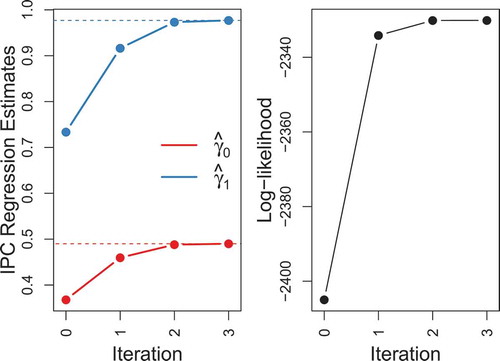
FIGURE 2 Demonstration of iterated IPC regression. 1000 individuals were sampled in equal shares from a two-group exponential distribution with group-specific rate parameters ${\lambda }_1=0.5$ and ${\lambda }_2=1.5$. Iterated IPC regression with a dummy variable indicating grouping was used to estimate the group difference in the rate parameter. On the left side, initial and re-estimated IPC regression estimates are shown. Red dots are estimates of ${\lambda }_1$ and blue dots are estimates of the difference ${\lambda }_2-{\lambda }_1$. Dashed lines mark the corresponding maximum likelihood estimates. Clearly, the initial IPC regression estimates are biased. After just two iterations, however, the iterated IPC regression estimates approach the corresponding maximum likelihood estimates. The log-likelihood function is shown on the right side. The iterative reduction of the bias in the IPC regression estimates leads to an increase of the log-likelihood.

The iterated IPC algorithm converges if the change in either the IPC regression estimates or in the log-likelihood becomes negligibly small. Unfortunately, the algorithm does not always converge. Especially, if the true individual- or group-specific value of a parameter lies close to (or at) the border of its parameter space, the algorithm might go awry. However, given strong heterogeneity in a sample, we observed across various models that the iterations often yield substantial improvement over the initial IPC regression estimates before breaking down. Therefore, the iteration with the largest log-likelihood might be preferred to the initial results.

We would like to note two more observations on the bias correction procedure. First, IPC regression estimates are unbiased in homogeneous samples and therefore cannot be further improved by updating the IPCs. If iterated IPC regression is used in a homogeneous sample, the algorithm will overfit the estimates to random fluctuation of the data. In this case, the resulting estimates can be marginally worse than the initial estimates, but the difference will be inconsequential for most practical purposes. Second, updating the IPCs comes at the cost of additional computational demands. In our experience, however, the algorithm usually converges quickly within few iterations. Even for samples with a few thousand individuals and models with more than 30 parameters, updating the IPCs took less than a minute with a standard desktop PC.

Software implementation

IPC regression is implemented as a package for the statistical programming language R (R Core Team, 2019), termed ipcr. The ipcr package makes it easy for researchers to study heterogeneity in the parameter estimates of an SEM fitted with the OpenMx package (Neale et al., 2015). The ipcr package performs “vanilla”, IPC regression as introduced by Oberski (2013) as well as iterated IPC regression. More information of how the ipcr package can be installed and used can be found under https://github.com/manuelarnold/ipcr/.

Monte Carlo simulations

To evaluate the performance of vanilla and iterated IPC regression to detect and estimate heterogeneity in dynamic panel models in discrete and continuous time we conducted the following two Monte Carlo simulations. The first simulation aims to substantiate our theoretical considerations regarding the bias for bivariate dynamic panel models. The second simulation investigates whether IPC regression provides valid inferences and compares the power of the method with MGSEM. Additional simulations to evaluate the performance of IPC regression for non-normally distributed data, more periods, and a comparison to a multilevel model, an MGSEM, and an SEM tree are provided as Online Supplemental Material.

Simulation I: Demonstration of the bias

In the following simulation studies, we used the discrete-time dynamic panel model depicted in Figure 1 with five measurement waves as a simulation model. The data were sampled from a multivariate normal distribution with two distinct sets of parameter values. 125 observations were generated per group, resulting in a pooled sample with 250 observations in total. A discrete-time and a continuous-time dynamic panel model were fitted to the same data, ignoring the group differences. Then, we used vanilla and iterated IPC regression with a dummy variable to recover the group differences in the parameter values of the dynamic panel models. Iterated IPC regression was performed by re-estimating the IPC regression parameters until the change in all parameters was smaller than 0.0001. We repeated this procedure 10,000 times.

The discrete-time population parameter values used to generate the data are shown in the upper half of Table 1, separated for both groups. For easy reference, we transformed these parameter values into continuous time and printed them in the lower half of the table. As clearly apparent from Table 1, group 1 and 2 differ substantively. The first group is characterized by strong autoregressive coefficients and no cross-lagged effects, whereas the second group exhibits substantial cross-lagged effects and smaller autoregressive coefficients. In addition, the variance of $x$ and $y$ was chosen twice as high for the second group as compared to the first.

TABLE 1 Group-specific Population Parameter Values for the Dynamic Panel Models in Discrete and Continuous Time

Time	$\theta$	Group 1	Group 2	$\theta$	Group 1	Group 2
Discrete	${\beta }_{xx}$	0.700	0.450	${\varphi }_{yx}$	0.300	1.000
	${\beta }_{yx}$	0.000	0.300	${\varphi }_{yy}$	1.000	2.000
	${\beta }_{xy}$	0.000	0.300	${\psi }_{xx}$	0.510	1.145
	${\beta }_{yy}$	0.700	0.450	${\psi }_{yx}$	0.153	0.168
	${\varphi }_{xx}$	1.000	2.000	${\psi }_{yy}$	0.510	1.145
Continuous	$a_{xx}$	– 0.357	– 1.092	${\varphi }_{yx}$	0.300	1.000
	$a_{yx}$	0.000	0.805	${\varphi }_{yy}$	1.000	2.000
	$a_{xy}$	0.000	0.805	$q_{xx}$	0.713	2.760
	$a_{yy}$	– 0.357	– 1.092	$q_{yx}$	0.214	– 1.034
	${\varphi }_{xx}$	1.000	2.000	$q_{yy}$	0.713	2.760

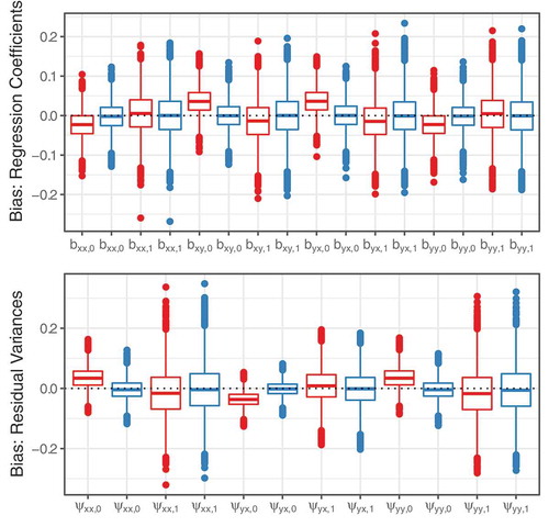
We will first discuss the results for the discrete-time dynamic panel model. As expected from the theoretical example, both IPC regression methods provided accurate estimates of heterogeneity in the initial variance and covariance parameters. Further, IPC regression estimates for regression coefficients and dynamic error term variance parameters were slightly distorted. Figure 3 depicts boxplots visualizing the bias of the IPC methods for regression coefficients (top graph) and dynamic error term variance parameters (lower graph). The estimates of vanilla IPC regression are printed in red and estimates after updating the IPCs are depicted in blue. Boxplots whose median lines lie close to the dotted black line indicate that the corresponding IPC regression estimates were approximately unbiased. Using the vanilla method, the intercepts (marked with the subscript $0$) of the IPC regression equations were more biased than the slopes (subscript $1$). Our updated IPC method erased the bias in the intercepts and provided accurate estimates for all types of model parameters. Averaged over all parameters, the root mean squared error of iterated IPC regression (RMSE = 0.089) was slightly smaller than the one of the vanilla procedure (RMSE = 0.094).

FIGURE 3 Boxplots of the bias of the IPC regression estimates for the discrete-time dynamic panel model. Red: vanilla IPC regression, blue: iterated IPC regression.

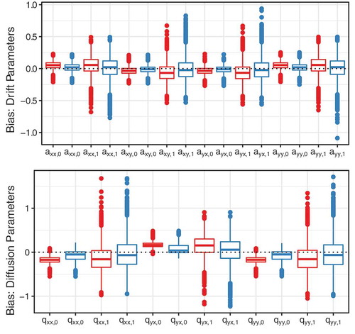
The performance of the IPC regression methods for the continuous-time dynamic model was similar to the findings for the discrete-time parameters above. The estimates for the initial variance and covariance parameters provided by both IPC regression methods were near the true values, whereas estimates for the remaining model parameters were biased. Figure 4 presents the bias in the IPC regression estimates for drift and diffusion parameters. Overall, the IPC regression estimates showed more variability for the continuous-time parameters than for the discrete-time parameters. As for the discrete-time model, vanilla IPC regression exhibited a slight bias. Re-estimating the IPCs with our correction procedure reduced this bias at the cost of increased variability of the IPC regression estimates. Moreover, the iterated IPC algorithm converged only in 53.78% of the trials and fell back to the starting values or an intermediate solution in the remaining trials. Nevertheless, in terms of the RMSE averaged over all parameters, iterated IPC regression (RMSE = 0.168) slightly outperformed vanilla IPC regression (RMSE = 0.174).

FIGURE 4 Boxplots of the bias of the IPC regression estimates for the continuous-time dynamic panel model. Red: vanilla IPC regression, blue: iterated IPC regression.

Simulation II: Statistical power and false positive rate

In the second simulation, we investigated the power of IPC regression to detect a difference in a parameter value and the false positive rate in case of homogeneous parameters. We generated multivariate normal data from bivariate dynamic panel models with five measurement occasions. We specified the population models in a way that only the cross-lagged effects from the variable $x$ on $y$ differed slightly between two groups. All other parameters were equal. In contrast to the previous simulation, we used different population models for the discrete- and continuous-time models. The corresponding parameter values for both population models (shown in Table 2) resulted in similar but not identical population covariance matrices. After a data set was generated, a pooled dynamic panel model was fitted, and parameter heterogeneity was tested with IPC regression (vanilla and iterated) using a dummy variable. We used the same convergence criterion for iterated IPC regression as in the previous simulation. We investigated power and false positive rate for group sizes of 100, 125, 150, 175, and 200 resulting in total sizes of 200, 250, 300, 350, and 400. For each sample size, we replicated this process 10,000 times.

TABLE 2 Population Parameter Values for the Dynamic Panel Models Used in Simulation II.

Discrete time				Continuous time
$\theta$	Value	$\theta$	Value	$\theta$	Value	$\theta$	Value
${\beta }_{xx}$	0.500	${\varphi }_{yx}$	0.300	$a_{xx}$	– 0.780	${\varphi }_{yx}$	0.300
${\beta }_{yx}$	0.200/0.300	${\varphi }_{yy}$	1.000	$a_{yx}$	0.424/0.546	${\varphi }_{yy}$	0.300
${\beta }_{xy}$	0.200	${\psi }_{xx}$	0.650	$a_{xy}$	0.424	$q_{xx}$	1.306
${\beta }_{yy}$	0.500	${\psi }_{yx}$	0.013	$a_{yy}$	– 0.780	$q_{yx}$	– 0.379
${\varphi }_{xx}$	1.000	${\psi }_{yy}$	0.650	${\varphi }_{xx}$	1.000	$q_{yy}$	1.306

Note. That the cross-lagged effects ${\beta }_{yx}$ and $a_{yx}$ differ between the two groups.

As a reference, we compared the power of the IPC regression methods to the power of MGSEM. Although MGSEM lacks the flexibility and computational simplicity of IPC regression, in simple (single-variable) group comparisons with correctly specified models, standard maximum-likelihood theory suggests it should provide the uniformly most powerful test. MGSEM therefore presents a good gold standard reference for these cases. The MGSEMs were specified by letting only the cross-lagged effects of $x$ on $y$ differ between groups. We computed the power of the MGSEMs by conducting likelihood ratio tests that compared the fit of the MGSEMs to the fit of the pooled models.

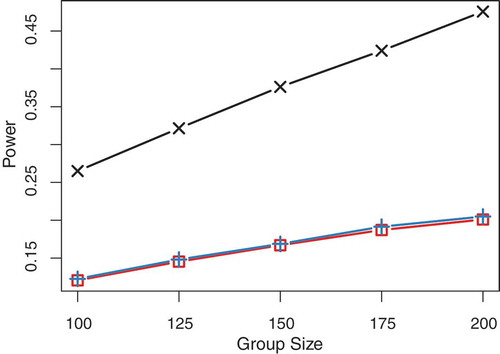
Figure 5 shows the power of IPC regression for the discrete-time model. Depicted is the rejection rate of the null hypothesis that the cross-lagged effects from $x$ on $y$ are equal in both groups, plotted against the number of individuals for a significance level of 5%. Red lines refer to the power of vanilla IPC regression, blue lines to iterated IPC regression, and black lines mark the power of MGSEM. For the discrete-time model, the IPC regression methods appeared to be on average 3.97 percentage points (range: [3.03, 5.30]) less powerful than MGSEM. Iterated IPC regression achieved a marginally larger power with a difference of 0.66 percentage points (range: [0.35, 0.94]). The power for the continuous-time model is presented in Figure 6. We found that the difference in power between the IPC regression methods and MGSEM were substantively larger for the continuous-time model than for the discrete-time model. On average, the power of the IPC regression was 20.68 percentage points (range: [14.25, 27.47]) smaller than the power of MGSEM. In addition, the power of IPC regression appeared to grow more slowly as a function of sample size. Again, iterated IPC appeared slightly more powerful than vanilla IPC regression (average difference: 0.28, range: [0.17, 0.44]).

FIGURE 5 Power to detect that the population group difference in the cross-lagged effect ${\beta }_{yx}$ of the discrete-time model is non-zero. Black crosses: MGSEM, red squares: vanilla IPC regression, blue pluses: iterated IPC regression.

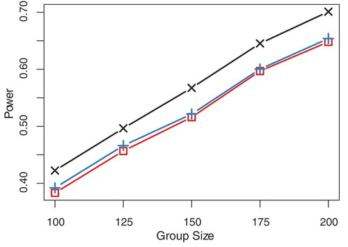
FIGURE 6 Power to detect that the population group difference in the drift parameter $a_{yx}$ of the continuous-time model is non-zero. Black crosses: MGSEM, red squares: vanilla IPC regression, blue pluses: iterated IPC regression.

Besides power, the false detection rate of the IPC regression methods is of great importance for drawing correct conclusions from the data. We assessed the type I error rate for population parameters that are identical in the two groups for a significance level of 5%. We summarized the results by averaging the type I error rate for the three parameter types in the models (initial variance, regression coefficient/drift, dynamic error term variance/diffusion). Table 3 shows the proportions of type I errors for the discrete-time model and Table 4 for the continuous-time model. In line with simulation results from Oberski (2013), the type I error rates were close to 5% for most parameters. Iterated IPC regression committed slightly more type I errors for regression and drift parameters. These findings imply that the standard errors of iterated IPC regression for regression/drift parameters were slightly too small and could explain why iterated IPC regression appeared marginally more powerful to detect heterogeneity.

TABLE 3 Proportions of Type I Errors for the Parameters Estimates of the Discrete-time Dynamic Panel Model

	Vanilla IPC			Iterated IPC
Group size	$\beta$	$\varphi$	$\psi$	$\beta$	$\varphi$	$\psi$
100	5.483	5.047	5.353	6.097	5.047	5.437
125	5.167	5.163	5.133	5.663	5.163	5.277
150	5.037	5.143	5.010	5.500	5.143	5.207
175	5.173	4.940	5.150	5.600	4.940	5.090
200	5.093	4.900	4.850	5.443	4.900	4.983

TABLE 4 Proportions of Type I Errors for the Parameters Estimates of the Continuous-time Dynamic Panel Model

	Vanilla IPC			Iterated IPC
Group size	$a$	$\varphi$	$q$	$a$	$\varphi$	$q$
100	5.333	5.083	5.353	5.250	5.083	4.477
125	5.103	5.007	5.263	5.183	5.007	4.620
150	5.207	5.090	5.143	5.247	5.090	4.657
175	5.077	5.193	4.993	5.157	5.193	4.580
200	4.810	5.207	4.803	4.920	5.207	4.463

In contrast to Simulation I, there was not a single case of non-convergence of the iterated IPC regression algorithm in Simulation II. This finding suggests that the convergence problems for the continuous-time dynamic panel model were mainly driven by the larger group differences used in the previous simulation.

Discussion

The present study investigated the performance of IPC regression (Oberski, 2013) to identify and estimate parameter heterogeneity in dynamic panel models. Overall, we found that IPC regression is a promising method to identify and estimate individual or group differences. In comparison to other contemporary approaches formally addressing heterogeneity with covariates, IPC regression offers a general framework that encompasses all types of SEMs and covariates and makes identifying and explaining individual differences as simple, flexible, and fast as linear regression.

IPC regression was evaluated in terms of bias in the recovery of true group differences, the power to detect parameter heterogeneity, and the type I error rate for homogeneous parameters. By means of a theoretical example and through Monte Carlo simulations, we demonstrated that original, “vanilla”, IPC regression estimates can be slightly biased due to large differences in regression parameters. Additional heterogeneity in variance parameters may amplify this bias. As a rule of thumb, the bias seems to affect mainly parameters connected to endogenous variables like regression and residual variance parameters, whereas the IPC regression estimates for parameters associated with exogenous variables such as the initial variance parameters remain comparatively unbiased. Hence, IPC regression may perform worse for SEMs with many directed paths such as dynamic panel models than for models with few directed paths such as CFA models. This argument would also explain why Oberski (2013) found nearly unbiased estimates of group differences in a CFA model.

To correct the bias in vanilla IPC regression, we introduced a novel updating procedure, which we termed iterated IPC regression. Iterated IPC regression produced approximately unbiased estimates of group differences in the parameters of a discrete-time dynamic panel model and outperformed vanilla IPC regression in terms of the RMSE. For the continuous-time dynamic panel model, however, iterated IPC regression corrected the bias but at the cost of adding additional variability to the estimates. Nevertheless, updating the IPCs still improved the estimates on average as indicated by a smaller RMSE.

In situations in which MGSEM could be applied as an alternative to IPC regression, we compared the power of IPC regression to that of MGSEM, which theory suggests is uniformly most-powerful in these cases. IPC regression yielded power only slightly below that of this theoretically optimal method to detect group differences in the cross-lagged effect of a discrete-time dynamic panel model. For the continuous-time model, however, IPC regression was no more than half as powerful as MGSEM. It should be noted that MGSEM cannot be applied to all scenarios allowed by IPC regression; for example, MGSEM does not investigate partial effects of multiple covariates of model parameters. In agreement with earlier theoretical findings, both IPC regression methods did control the type I error rate accurately.

In summary, our findings demonstrate that (iterated) IPC regression is a useful tool to study heterogeneity in discrete-time dynamic panel model. For continuous-time dynamic panel models, however, our findings were mixed: high variance caused by the bias correction procedure and a small power make (iterated) IPC regression unappealing especially in smaller data sets. We believe that these problems are caused by non-linear parameter constraints and high correlation between parameter estimates of the continuous-time dynamic panel model. Considering these difficulties, IPC regression seems more appropriate for models that can be parameterized without non-linear constraints such as the discrete-time dynamic panel model or other contemporaneous models for longitudinal data such as latent growth curve models (Bollen & Curran, 2006) or latent change score models (McArdle, 2001), if these models are applicable.

Although IPC regression is a general, easy to use, and flexible approach to detect parameter heterogeneity, we want to stress that it is not always the most appropriate one. Depending on a study’s objective, other methods for addressing heterogeneity should be preferred to IPC regression. For example, multilevel models are like an obvious choice in situations where it is sufficient to allow for varying parameter values between individuals and there is no interest in explaining these differences. In contrast, if a study aims to test differences between few known groups in the data (e.g., in variance parameters), MGSEM will often be the better choice. If a study’s goal is to determine homogeneous groups in the data with help of additionally observed covariates, partitioning methods like SEM trees or forests often are better suited for the task, in particular if computation time is not an issue.

In the following, we will briefly touch upon some limitations of IPC regression that researchers should consider. First, the usefulness of IPC regression depends on the covariates available. If none of the additional covariates is related to individual or group differences in the parameters, IPC regression will fail to detect the source of heterogeneity. In cases of unobserved group membership, researchers may want to resort to methods like finite mixture models (Jedidi, Jagpal, & DeSarbo, 1997; Lubke & Muthén, 2005; Muthén & Shedden, 1999). Second, IPC regression is a data-driven or exploratory procedure and therefore susceptible to capitalize on chance characteristics of the data (MacCallum, Roznowski, & Necowitz, 1992). Modifying models by blindly following the advice of IPC regression may lead to a model that works well in the observed sample but does not generalize to others. We thus recommend paying not only close attention to the $p$-value provided by IPC regression, but also to the size of the estimated individual or group difference. See also Saris, Satorra, and van der Veld (2009), for a related discussion about model modification using the modification index and expected parameter change. Third, using IPC regression to investigate the effect of a large number of covariates on complex models with many parameters will yield a large number of IPC regression estimates that can be challenging to interpret. Regularization techniques such as lasso (Tibshirani, 1996) could be used to find a subset of the most important covariates.

In summary, however, we believe that IPC regression is a useful tool to investigate parameter heterogeneity in SEMs for longitudinal data such as dynamic panel models that combines flexibility with its unique computational simplicity.

Acknowledgement

We acknowledge support by the Open Access Publication Fund of Humboldt-Universität zu Berlin.

Notes

¹ The biased estimate of the sample covariance is used.

Appendix

Expressing IPC Regression Estimates with Group-specific Estimates

In the following, we express the IPC regression estimates ${\hat{\gamma }}_0$ and ${\hat{\gamma }}_1$ in terms of the group-specific maximum likelihood estimates ${\hat{\lambda }}_1$ and ${\hat{\lambda }}_2$ as shown in Equations (26(26) ${\hat{\gamma }}_0=\frac{4{\hat{\lambda }}_1^2{\hat{\lambda }}_2}{{\left({\hat{\lambda }}_1+{\hat{\lambda }}_2\right)}^2}$(26) ) and (27(27) ${\hat{\gamma }}_1=\frac{4{\lambda }_1{\lambda }_2\left({\hat{\lambda }}_2-{\hat{\lambda }}_1\right)}{{\left({\hat{\lambda }}_1+{\hat{\lambda }}_2\right)}^2}$(27) ). Note that ${\hat{\gamma }}_0$ and ${\hat{\gamma }}_1$ are simple ordinary least squares estimates given by ${\hat{\gamma }}_1=s_{\mathrm{I}\mathrm{P}\mathrm{C},z}/s_z^2$ and ${\hat{\gamma }}_0=\overline{\mathrm{I}\mathrm{P}\mathrm{C}}-{\hat{\gamma }}_1\bar{z}$, where $s_{\mathrm{I}\mathrm{P}\mathrm{C},z}$ is the sample covariance between the IPCs and the covariate $z_i$, $s_z^2$ is the sample variance of the covariate, and $\overline{\mathrm{I}\mathrm{P}\mathrm{C}}$ and $\bar{z}$ are the sample means of the IPCs and the covariate, respectively.

Following Equation (16)(16) $\mathcal{I}\mathcal{P}\mathcal{C}(\hat{\theta };{\mathbf{y}}_i)=\hat{\theta }+\mathcal{I}(\hat{\theta }{)}^{-1}\mathcal{S}(\hat{\theta };{\mathbf{y}}_i)$(16) , the IPC of individual $i$ is given by

$\mathcal{I}\mathcal{P}\mathcal{C}(\hat{\lambda };y_i)=\hat{\lambda }+\mathcal{I}(\hat{\lambda }{)}^{-1}\mathcal{S}(\hat{\lambda };y_i)=\hat{\lambda }+{\hat{\lambda }}^2\left(\frac{1}{\hat{\lambda }}-y_i\right)=2\hat{\lambda }-{\hat{\lambda }}^2{y}_i.$

Next, we express the pooled maximum likelihood estimate $\hat{\lambda }$ as a function of the group-specific maximum likelihood estimates:

$\begin{array}{rl}& \hat{\lambda }={\left(\frac{1}{n}\sum _{i=1}^n{y}_i\right)}^{-1}={\left[\frac{1}{n}\left(\frac{n_1}{n_1}\sum _{i=1}^{n_1}{y}_i+\frac{n_2}{n_2}\sum _{i=n_1+1}^n{y}_i\right)\right]}^{-1}\\ & ={\left[\frac{1}{n}\left(\frac{n_1}{{\hat{\lambda }}_1}+\frac{n_2}{{\hat{\lambda }}_2}\right)\right]}^{-1}\stackrel{n_1=n_2=\frac{n}{2}}{=}{\left(\frac{1}{2{\hat{\lambda }}_1}+\frac{1}{2{\hat{\lambda }}_2}\right)}^{-1}=\frac{2{\hat{\lambda }}_1{\hat{\lambda }}_2}{{\hat{\lambda }}_1+{\hat{\lambda }}_2}\end{array}$

Using both equations from above, the IPC regression slope ${\hat{\gamma }}_1$ can be written in terms of the group-specific maximum likelihood estimates:

$\begin{array}{rl}& {\hat{\gamma }}_1=\frac{s_{\mathrm{I}\mathrm{P}\mathrm{C},z}}{s_z^2}\\ & =\frac{\sum _{i=1}^n{z}_i\mathrm{I}\mathrm{P}\mathrm{C}(\hat{\lambda };y_i)-\frac{1}{n}\sum _{i=1}^n{z}_i\sum _{i=1}^n\mathrm{I}\mathrm{P}\mathrm{C}(\hat{\lambda };y_i)}{\sum _{i=1}^n{z}_i^2-\frac{1}{n}{\left(\sum _{i=1}^n{z}_i\right)}^2}\\ & =\frac{\sum _{i=n_1+1}^n\left(2\hat{\lambda }-{\hat{\lambda }}^2{y}_i\right)-\frac{n_2}{n}\sum _{i=1}^n\left(2\hat{\lambda }-{\hat{\lambda }}^2{y}_i\right)}{\frac{n_{2}n-n_2^2}{n}}\\ & =\frac{-n{\hat{\lambda }}^2\sum _{i=n_1+1}^n{y}_i+n_2{\hat{\lambda }}^2\sum _{i=1}^n{y}_i}{n_{2}n-n_2^2}\\ & \stackrel{n=n_1+n_2}{=}\frac{{\hat{\lambda }}^2\left(-n_1\sum _{i=n_1+1}^n{y}_i-n_2\sum _{i=n_1+1}^n{y}_i+n_2\sum _{i=1}^n{y}_i\right)}{n_1{n}_2}\\ & ={\hat{\lambda }}^2\left(\frac{1}{n_1}\sum _{i=1}^{n_1}{y}_i-\frac{1}{n_2}\sum _{i=n_1+1}^n{y}_i\right)={\hat{\lambda }}^2\left(\frac{1}{{\hat{\lambda }}_1}-\frac{1}{{\hat{\lambda }}_2}\right)\\ & ={\left(\frac{2{\hat{\lambda }}_1{\hat{\lambda }}_2}{{\hat{\lambda }}_1+{\hat{\lambda }}_2}\right)}^2\frac{{\hat{\lambda }}_2-{\hat{\lambda }}_1}{{\hat{\lambda }}_1{\hat{\lambda }}_2}=\frac{4{\lambda }_1{\lambda }_2\left({\hat{\lambda }}_2-{\hat{\lambda }}_1\right)}{{\left({\hat{\lambda }}_1+{\hat{\lambda }}_2\right)}^2}\end{array}$

Finally, we can derive the IPC regression intercept ${\hat{\gamma }}_0$ in the same way

$\begin{array}{rl}{\hat{\gamma }}_0& =\overline{\mathrm{I}\mathrm{P}\mathrm{C}}-{\hat{\gamma }}_1\bar{z}\\ & =\frac{1}{n}\sum _{i=1}^n\mathrm{I}\mathrm{P}\mathrm{C}(\hat{\lambda };y_i)-{\hat{\gamma }}_1\frac{1}{n}\sum _{i=1}^n{z}_i\\ & =\frac{1}{n}\sum _{i=1}^n\left(2\hat{\lambda }-{\hat{\lambda }}^2{y}_i\right)-{\hat{\lambda }}^2\left(\frac{1}{n_1}\sum _{i=1}^{n_1}{y}_i-\frac{1}{n_2}\sum _{i=n_1+1}^n{y}_i\right)\frac{n_2}{n}\\ & =2\hat{\lambda }+{\hat{\lambda }}^2\left(-\frac{1}{n}\sum _{i=1}^n{y}_i-\frac{n_2}{n_{1}n}\sum _{i=1}^{n_1}{y}_i+\frac{1}{n}\sum _{i=n_1+1}^n{y}_i\right)\\ & =2\hat{\lambda }+{\hat{\lambda }}^2\left(-\frac{1}{n}\sum _{i=1}^{n_1}{y}_i-\frac{n_2}{n_{1}n}\sum _{i=1}^{n_1}{y}_i\right)\\ & \stackrel{n=n_1+n_2}{=}2\hat{\lambda }-\frac{{\hat{\lambda }}^2}{n_1}\sum _{i=1}^{n_1}{y}_i=2\hat{\lambda }-\frac{{\hat{\lambda }}^2}{{\hat{\lambda }}_1}\\ & =2\frac{2{\hat{\lambda }}_1{\hat{\lambda }}_2}{{\hat{\lambda }}_1+{\hat{\lambda }}_2}-\frac{1}{{\hat{\lambda }}_1}{\left(\frac{2{\hat{\lambda }}_1{\hat{\lambda }}_2}{{\hat{\lambda }}_1+{\hat{\lambda }}_2}\right)}^2=\frac{4{\hat{\lambda }}_1^2{\hat{\lambda }}_2}{{\left({\hat{\lambda }}_1+{\hat{\lambda }}_2\right)}^2}\end{array}$

References

- Allison, P. D., Williams, R., & Moral-Benito, E. (2017). Maximum likelihood for cross-lagged panel models with fixed effects. Socius, 3, 1–17. doi:10.1177/2378023117710578
- Biesanz, J. C. (2012). Autoregressive longitudinal models. In R. H. Hoyle (Ed.), Handbook of structural equation modeling (pp. 459–471). New York, NY: Guilford.
- Bollen, K. A. (1989). Structural equations with latent variables. New York, NY: Wiley.
- Bollen, K. A., & Brand, J. E. (2010). A general panel model with random and fixed effects: A structural equations approach. Social Forces, 89, 1–34. doi:10.1353/sof.2010.0072
- Bollen, K. A., & Curran, P. J. (2006). Latent curve models: A structural equation perspective. Hoboken, NJ: John Wiley & Sons.
- Brandmaier, A. M., Driver, C. C., & Voelkle, M. C. (2018). Recursive partitioning in continuous time analysis. In K. van Montfort, J. H. L. Oud, & M. C. Voelkle (Eds.), Continuous time modeling in the behavioral and related sciences (pp. 259–282). New York, NY: Springer.
- Brandmaier, A. M., Prindle, J. J., McArdle, J. J., & Lindenberger, U. (2016). Theory-guided exploration with structural equation model forests. Psychological Methods, 21, 566–582. doi:10.1037/met0000090
- Brandmaier, A. M., von Oertzen, T., McArdle, J. J., & Lindenberger, U. (2013). Structural equation model trees. Psychological Methods, 18, 71–86. doi:10.1037/a0030001
- Brown, T. A. (2006). Confirmatory factor analysis for applied research. New York, NY: Guilford.
- Demidenko, E. (2013). Mixed models: Theory and applications with R (2nd ed.). Hoboken, NJ: Wiley.
- Driver, C. C., & Voelkle, M. C. (2018). Hierarchical Bayesian continuous time dynamic modeling. Psychological Methods, 23, 774–779. doi:10.1037/met0000168
- George, M. R. W., Yang, N., Jaki, T., Feaster, D. J., Lamont, A. E., Wilson, D. K., & van Horn, M. L. (2013). Finite mixtures for simultaneously modelling differential effects and non-normal distributions. Multivariate Behavioral Research, 48, 816–844. doi:10.1080/00273171.2013.830065
- Granger, C. W. J. (1969). Investigating causal relations by econometric models and cross-spectral methods. Econometrica, 37, 424–438. doi:10.2307/1912791
- Halaby, C. N. (2004). Panel models in sociological research: Theory into practice. Annual Review of Sociology, 30, 507–544. doi:10.1146/annurev.soc.30.012703.110629
- Hamaker, E. L., Kuiper, R. M., & Grasman, R. P. P. P. (2015). A critique of the cross-lagged panel model. Psychological Methods, 20, 102–116. doi:10.1037/a0038889
- Hsiao, C. (2014). Analysis of panel data (3rd ed.). Cambridge, UK: University Press.
- Jedidi, K., Jagpal, H. S., & DeSarbo, W. S. (1997). Finite-mixture structural equation models for response-based segmentation and unobserved heterogeneity. Marketing Science, 16, 39–59. doi:10.1287/mksc.16.1.39
- Lubke, G. H., & Muthén, B. (2005). Investigating population heterogeneity with factor mixture models. Psychological Methods, 10, 21–39. doi:10.1037/1082-989X.10.1.21
- MacCallum, R. C., Roznowski, M., & Necowitz, L. B. (1992). Model modifications in covariance structure analysis: The problem of capitalization on chance. Psychological Bulletin, 111, 490–504. doi:10.1037/0033-2909.111.3.490
- Magnus, J. R., & Neudecker, H. (2019). Matrix differential calculus with applications in statistics and econometrics (3rd ed.). New York, NY: Wiley. doi:10.1002/9781119541219
- McArdle, J. J. (2001). A latent difference score approach to longitudinal dynamic structural analysis. In R. Cudeck, S. Du Toit, & D. Sörbom (Eds.), Structural equation modeling (pp. 341–380). Lincolnwood, IL: Scientific Software International.
- Merkle, E. C., Fan, J., & Zeileis, A. (2014). Testing for measurement invariance with respect to an ordinal variable. Psychometrika, 79, 569–584. doi:10.1007/s11336-013-9376-7
- Merkle, E. C., & Zeileis, A. (2013). Tests of measurement invariance without subgroups: A generalization of classical methods. Psychometrika, 78, 59–82. doi:10.1007/s11336-012-9302-4
- Muthén, B. O., & Shedden, K. (1999). Finite mixture modeling with mixture outcomes using the EM algorithm. Biometrics, 55, 463–469. doi:10.1111/j.0006-341X.1999.00463.x
- Neale, M. C., Hunter, M. D., Pritkin, J., Zahery, M., Brick, T. R., Kirkpatrick, R. M., … Boker, S. M. (2015). OpenMx 2.0: Extended structural equation and statistical modeling. Psychometrika, 81, 535–549. doi:10.1007/s11336-014-9435-8
- Neudecker, H., & Satorra, A. (1991). Linear structural relations: Gradient and Hessian of the fitting function. Statistics & Probability Letters, 11, 57–61. doi:10.1016/0167-7152(91)90178-T
- Oberski, D. L. (2013). A flexible method to explain differences in structural equation model parameters over subgroups. Retrieved from http://daob.nl/wp-content/uploads/2013/06/SEM-IPC-manuscript-new.pdf
- Oud, J. H. L. (2007). Continuous time modeling of reciprocal relationships in the cross-lagged panel design. In S. M. Boker & M. J. Wenger (Eds.), Data analytic techniques for dynamic systems in the social and behavioral sciences (pp. 87–129). Mahwah, NJ: Erlbaum.
- Oud, J. H. L., & Delsing, M. J. M. H. (2010). Continuous time modeling of panel data by means of SEM. In K. van Montfort, J. H. L. Oud, & A. Satorra (Eds.), Longitudinal research with latent variables (pp. 201–244). New York, NY: Springer.
- Oud, J. H. L., & Jansen, R. A. R. G. (2000). Continuous time state space modeling of panel data by means of SEM. Psychometrika, 65, 199–215. doi:10.1007/BF02294374
- R Core Team. (2019). R: A language and environment for statistical computing. Vienna, Austria: R Foundation for Statistical Computing. Retrieved from https://www.R-project.org/
- Saris, W. E., Satorra, A., & Sörbom, D. (1987). The detection and correction of specification errors in structural equation models. Sociological Methodology, 17, 105–129. doi:10.2307/271030
- Saris, W. E., Satorra, A., & van der Veld, W. M. (2009). Testing structural equation models or detection of misspecifications? Structural Equation Modeling, 16, 561–582. doi:10.1080/10705510903203433
- Satorra, A. (1989). Alternative test criteria in covariance structure analysis: A unified approach. Psychometrika, 54, 131–151. doi:10.1007/BF02294453
- Satorra, A. (1992). Asymptotic robust inferences in the analysis of mean and covariance structures. Sociological Methodology, 22, 249–278. doi:10.2307/270998
- Savalei, V. (2014). Understanding robust corrections in structural equation modeling. Structural Equation Modeling, 21, 149–160. doi:10.1080/10705511.2013.824793
- Schuurman, N. K., Ferrer, E., de Boer-Sonnenschein, M., & Hamaker, E. L. (2016). How to compare cross-lagged associations in a multilevel autoregressive model. Psychological Methods, 21, 206–221. doi:10.1037/met0000062
- Singer, J. D., & Willet, J. B. (2003). Applied longitudinal data analysis. Oxford, UK: Oxford University Press.
- Sörbom, D. (1974). A general method for studying differences in factor means and factor structure between groups. British Journal of Mathematics and Statistical Psychology, 27, 229–239. doi:10.1111/j.2044-8317.1974.tb00543.x
- Sörbom, D. (1989). Model modification. Psychometrika, 54, 371–384. doi:10.1007/BF02294623
- Tibshirani, R. (1996). Regression shrinkage and selection via the lasso. Journal of the Royal Statistical Society, 58, 267–288. doi:10.1111/rssb.1996.58.issue-1
- Usami, S., Hayes, T., & McArdle, J. (2017). Fitting structural equation model trees and latent growth curve mixture models in longitudinal designs: The influence of model misspecification. Structural Equation Modeling, 24, 585–598. doi:10.1080/10705511.2016.1266267
- van Montfort, K., Oud, J. H. L., & Voelkle, M. C. (2018). Continuous time modeling in the behavioral and related sciences. New York, NY: Springer.
- Voelkle, M. C., Oud, J. H. L., Davidov, E., & Schmidt, P. (2012). An SEM approach to continuous time modeling of panel data: Relating authoritarianism and anomia. Psychological Methods, 17, 176–192. doi:10.1037/a0027543
- Voelkle, M. C., Oud, J. H. L., von Oertzen, T., & Lindenberger, U. (2012). Maximum likelihood dynamic factor modeling for arbitrary N and T using SEM. Structural Equation Modeling, 19, 329–350. doi:10.1080/10705511.2012.687656
- Wang, T., Merkle, E. C., & Zeileis, A. (2014). Score-based tests of measurement invariance: Use in practice. Frontiers in Psychology, 5, 438. doi:10.3389/fpsyg.2014.00438
- Wang, T., Strobl, C., Zeileis, A., & Merkle, E. C. (2018). Score-based tests of differential item functioning via pairwise maximum likelihood estimation. Psychometrika, 83, 132–155. doi:10.1007/s11336-017-9591-8
- White, H. (1984). Asymptotic theory for econometricians. Orlando, FL: Academic Press.
- Yuan, K.-H., & Bentler, P. M. (2007). Structural equation modeling. In C. R. Rao & S. Sinharay (Eds.), Handbook of statistics (Vol. 26, pp. 297–358). Amsterdam, Netherlands: North Holland.
- Zeileis, A. (2005). A unified approach to structural change tests based on ML scores, F statistics, and OLS residuals. Econometric Reviews, 24, 445–466. doi:10.1080/07474930500406053
- Zeileis, A., & Hornik, K. (2007). Generalized M-fluctuation tests for parameter instability. Statistica Neerlandica, 61, 488–508. doi:10.1111/stan.2007.61.issue-4
- Zyphur, M. J., Allison, P. D., Tay, L., Voelkle, M. C., Preacher, K. J., Zhang, Z., … Diener, E. (2019). From data to causes I: Building a general cross-lagged panel model (GCLM). Organizational Research Methods. Advance online publication. doi:10.1177/1094428119847278
- Zyphur, M. J., Voelkle, M. C., Tay, L., Allison, P. D., Preacher, K. J., Zhang, Z., … Diener, E. (2019). From data to causes II: Comparing approaches to panel data analysis. Organizational Research Methods. Advance online publication. doi:10.1177/1094428119847280