Characterisation of liquid food colour from digital images

ABSTRACT

The characteristic colour of translucent liquid foods is defined as the colour values at infinite depth, where the liquid depth and the background effects are surpassed. A measurement cell with variable depth was built, and the L*a*b* colour was measured from digital images. Colour versus depth was fitted to an exponential equation, from which the characteristic colour was obtained. Thirteen different liquids were tested with this methodology and compared with spectrophotometer measurements. The average total colour difference between approaches was 50.85 ± 18.89. Image analysis led to more realistic predictions, and a high correlation between Hue angle values was obtained for most samples, with the exception of only one.

KEYWORDS:

• Beverages
• Colour
• Food property
• Food quality
• Image analysis

Introduction

The colour of foods is a meaningful feature since it is one of the first characteristics to be evaluated by the consumers, closely associated with the food quality.^[1,2] In general, it is a complex sensation which depends, among several factors, on the consumer’s perception, the chemical composition of the food, and the incident light. All those factors indicate that the colour is not only an intrinsic property of the sample but also it is influenced by the environment.^[2] In food technology, the colour is commonly expressed in the CIELAB or CIE 1976 L*a*b* colour space,^[3] where L* is the lightness, a* is the redness (from green to red), and b* is the yellowness (from blue to yellow). This is often determined using colorimeters,^[2] which measure the reflected light from a surface under standard lighting conditions. These measurements can be easily performed for opaque solid foods, where most of the light is reflected by the food surface.On the other hand, the colour of transparent or translucent foods, like beverages, is much more complex to define and measure. Aside from the influence of subjectivity on the consumer perception, the colour of translucent foods is greatly affected by the liquid’s depth and the scene background. Up to the present, the colour of translucent liquids is usually determined using spectrophotometers, which measure the absorbance or transmittance spectrum, from which CIELAB colour space information can be obtained.^[4] These devices use cells of different depths, and the effect of this variable in the colour value deserves to be studied. In this sense, Joubert^[5] measured the colour of rooibos tea with cells of different depths using a spectrophotometer. Huertas et al.^[6] measured the colour of wine samples with different thicknesses using a spectroradiometer and a spectrophotometer. González-Miret Martín et al.^[7] employed a spectroradiometer to measure colour of wines at different depths. Hernández et al.^[8] measured the wine colour at the centre and the rim of a normalised wine sampler using a spectroradiometer. Gómez-Robledo et al.^[9] measured the colour of virgin olive oil with cells of different thickness using a spectrophotometer and with cells of different diameters using a spectroradiometer. Carvalho et al.^[10] measured CIELAB colour of wines during ageing using a spectrophotometer.

On the other hand, the use of digital images to determine the colour of foods has been encouraged in the past few years,^[2] mainly for the surface colour of solid opaque foods. To measure colour from digital images, a computer vision system (CVS), consisting of a digital camera, an image acquisition ambient with controlled illumination and information processing software, is required.^[11] In these systems, one key step is the conversion of the Red, Green, and Blue (RGB) colour values obtained from digital cameras to the CIELAB colour space. However, only few works have been reported using this methodology regarding the colour of translucent liquid foods. González-Miret Martín et al.^[7] measured the colour of four commercial wines; Fernández-Vázquez et al.^[12] measured the colour of orange juice samples and discriminated between samples based on the measured colour and a trained sensory panel; both works used a commercial colour system, DigiEye (VeriVide, UK). Mendoza et al.^[13] explored the feasibility of a machine vision technique for predicting the quality of commercial canned beans, using colour and textural features extracted from drained beans and brine images. Hence, the objective of this work is to develop a simple methodology to obtain the characteristic colour of translucent liquid foods from digital images. With this aim, a measurement cell with variable depth was built, thus allowing the evaluation of depth influence on the colour in a single image. The digital images were processed to obtain L*, a*, and b* values from RGB information, using a standard colour chart and an empirical colour space conversion model. A software package was developed in MATLAB, as a graphical user interface, to process the images.

Material and methods

Measurement cell and characteristic colour

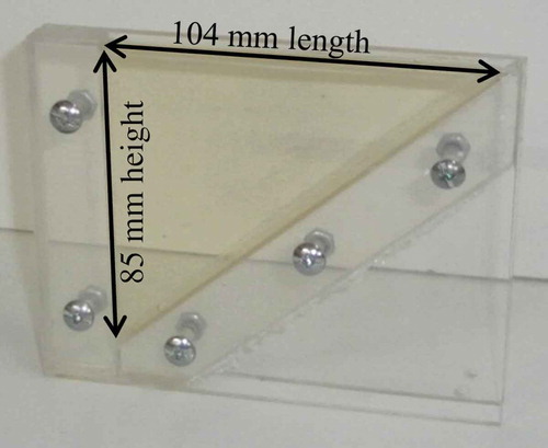
Diverse measurement cells or liquid container prototypes were designed, built, and tested. Finally, a transparent acrylic cell was employed, with its bottom painted in light grey (Fig. 1). The cell has 8 mm width, 104 mm length, and a tilted floor, so that its depth varies from 0 to 85 mm. To completely fill the cell, 35.4 cm³ of liquid are necessary.

Figure 1. Picture of the developed acrylic cell.

Both liquid depth and background affect colour measurement; therefore, it is necessary to consider them in order to provide a suitable description of the colour. As it was mentioned, the colour of liquids is defined as the colour at infinite depth. According to the Beer-Lambert law,^[14] an exponential function is proposed to represent the colour variation with depth (Eq. 1):

(1)

where C refers to each colour parameter, L*, a*, or b*, respectively. The subscript ‘0’ refers to the initial value (z = 0), β is related to the light absorption on the sample, and z is the liquid depth. As the cell depth increases (z → ∞), each colour parameter approaches a constant one, L*_∞, a*_∞, and b*_∞. Then, these values are defined as the characteristic colour of the sample. It is noteworthy that more general and detailed theories of light propagation on turbid media, as the Kubelka-Munk theory, are available,^[15] but nevertheless, a simple and empirical approach was chosen according to the aim of this work.

Image acquisition and processing

To obtain the digital images and then the colour of the samples, a CVS is required, which consists of an image acquisition chamber, a digital camera, and image processing software. In this work, the image acquisition was performed in a laboratory room with fluorescent lights, using a Samsung ST60 digital camera (automatic program, flash off, 3000 × 4000 pixels, ISO 100, white balance: white fluorescent).

Both the image processing and subsequent calculations were performed in a software package developed using MATLAB® (The Mathworks Inc., Natick, Mass., USA), as a graphics user interface (GUI) adapted from.^[16] This software, developed to measure the colour of solid foods, was previously tested and validated.^[17,18] Since the digital camera acquires images in the RGB colour space, a conversion to the CIELAB colour space must be applied. The direct conversion between these two colour spaces^[19,20] is suitable when standard illumination conditions are used. On the contrary, when the lighting is not standard, an empirical conversion must be performed, as it is stated in previous works regarding the measurement of the colour of the solid foods.^[21–26] These empirical models must be fitted by a calibration procedure using samples with known colour values. In this work, the following empirical conversion model was used, with linear and quadratic relations, as well as interactions between the RGB values:

(2)

The parameters α_i of this empirical conversion model were obtained using a X-Rite ColorChecker chart (X-Rite Inc., Grand Rapids, Michigan, USA), which is a standard reference used in several studies.^[23,25,27] It has 24 patches with different colours, with known L*a*b* values;^[28] in this work, D65 illuminant was considered. The error of the fitting procedure was assessed using the average total colour difference between L*, a*, and b* colour values of the ColorChecker and the predicted (Eq. 2) ones:

(3)

where subscripts F and R refer to fitted and reference values, respectively, and n refers to the number of ColorChecker patches (n = 24). The processing steps are summarised as follows:

1. Obtain an image of the cell filled with the sample.

2. Calibrate the colour space conversion model (Eq. 2).

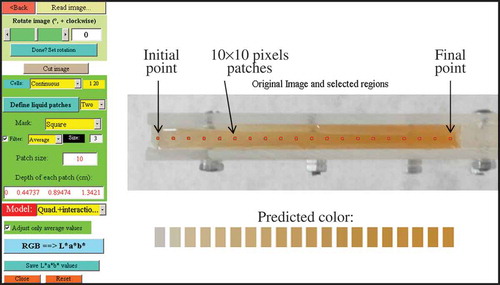
3. Select an initial and a final point in the liquid cell and define the number of intermediate points to use (see Fig. 2).

4. Obtain RGB values for each point. To diminish eventual noise, a small patch of several pixels was employed instead of using a single point (see Fig. 2).

5. Convert the RGB values to L*a*b* values for all the selected points, using Eq. (2).

6. Calculate the depth z for the selected points.

7. Finally, fit L*, a*, and b* values versus z (Eq. 1) to obtain C_∞, C₀, and β.

Figure 2. Image of the apple juice sample opened in the GUI. The 20 patches selected to measure colour versus depth are shown; the initial and final patches are indicated. Predicted RGB colours of these patches are also depicted.

The steps 2 to 7 are implemented in the developed software. The fitting performance of Eq. (1) was also expressed using the average total colour difference between measured and fitted colour values, for all depths, similarly to Eq. (3).

Samples and experimental measurements

Several fruit juices (grape, pear, multi-fruit, apple), wines (white, rosé, red), lager beer, and energy drinks of different colours (grapefruit, blue), purchased at a local market in La Plata (Argentina), were employed to test the proposed methodology. Also, selected liquid cleaners and deodorants of diverse colours were used; these samples were included since they are synthetic and present a more stable colour through time. All the samples were poured carefully in the cell, avoiding bubble formation; the beer sample was allowed to settle a few minutes until the bubbles disappeared. The camera was placed 25 cm above the sample, vertically aligned with the cell, and a single photograph was acquired for each measurement.

The L*a*b* colour of the whole set of samples was also estimated from spectral transmittance data^[29,30] in order to compare the performance of our methodology with that of the traditional method. For this, D65 standard illuminant and 2° standard observer were used, measuring between 380 nm and 780 nm at 1 nm interval (BECKMAN DU 650 Spectrophotometer, Brea, California, USA). A plastic cell of 1 cm depth was employed, using distilled water as reference. The Hue angle (Eq. 4) and Chroma (Eq. 5) were calculated from the L*a*b* values obtained by both approaches:

(4)

(5)

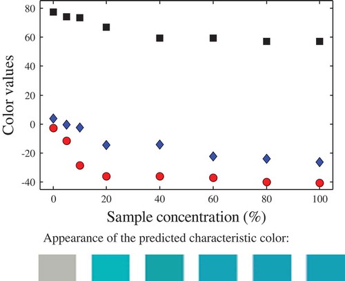
The ability of the developed methodology to detect concentration differences was determined by measuring the colour of two samples (blue energy drink and multi-fruit juice) diluted in distilled water. The final concentration of the diluted samples was 0, 5, 10, 20, 40, 60, and 80% (measured as sample volume/total volume). Additional measurements were performed to test the influence of the background on the characteristic colour. For this purpose, the cell floor was covered with plastic sheets of different colours (yellow, green, and black), and digital images with each background were acquired for a particular sample (blue energy drink). To analyse the influence of the background, a hypothesis test on the equality of means was done.^[31]

Results and discussion

Calibration of the conversion model

The first step before image processing is the calibration of the empirical model to transform colour spaces. As it can be seen in Eq. (2), the model’s response was linear on the parameters α_i, so the fitting was easily performed. It is worth mentioning that the digital camera used in this work automatically changes its setting from scene to scene, so the colour chart was always included in the scene. The average total colour difference between the ColorChecker values and the predicted (Eq. 2) L*, a*, and b* values was ΔE = 2.35 ± 0.27, considering the 13 samples detailed in Table 1.

Table 1. L*a*b* colour values obtained from image processing and from spectrophotometer measurements.

	Image processing			Spectrophotometer
Sample	L*∞	a*∞	b*∞	L*	a*	b*
Grape juice	82.71	−14.74	32.35	94.41	−2.33	7.99
Pear juice	84.87	−5.24	27.39	99.53	−0.48	2.10
Multi-fruit juice	68.49	30.58	46.37	80.99	9.17	17.88
Apple juice	59.67	25.31	61.25	96.77	−0.81	9.69
Grapefruit energy drink	82.81	−1.42	32.70	83.58	2.49	19.34
Blue energy drink	56.45	−39.98	−26.75	74.55	−17.87	3.48
Lager beer	47.18	37.18	56.62	93.70	−2.47	21.71
White wine	69.75	11.74	59.34	98.02	−1.40	9.03
Rosé wine	22.07	29.81	11.21	61.76	35.68	33.25
Red wine	12.53	3.54	−2.89	25.02	51.07	39.94
Green cleaner	20.82	−34.58	23.93	89.58	−27.02	30.76
Violet cleaner	25.73	38.24	−24.60	79.64	10.69	−15.59
Blue cleaner	33.28	−21.40	−32.42	93.17	−4.63	−3.80

Measurement of the characteristic colour

Figure 2 shows a digital image of an apple juice sample contained in the cell, as it is viewed in the developed GUI used to process the digital images. Also the predicted colours obtained from its processing are depicted. Two conversion steps were involved, so as to display the colours in a visual sense: first, the image is transformed from RGB space to L*a*b* using Eq. (2) and then from L*a*b* back to RGB values using a direct conversion model.^[3,19] As it can be seen, a good correlation is observed.

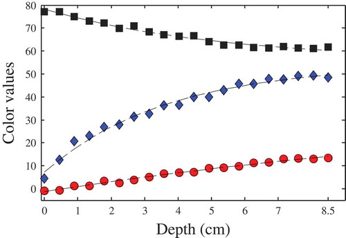
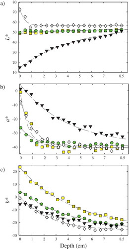
To define the characteristic colour, the dependence of the predicted colour values on the liquid depth was analysed. In this sense, Fig. 3 shows the L*, a*, and b* colour values versus the liquid depth. From these results, it is clear that as the depth increases, each colour value approaches a constant one. These colour values were used to fit Eq. (1) of this work. For this particular sample, the average total colour difference of the fitting procedure was ΔE = 2.09 ± 0.69, using the 20 patches showed in Fig. 2. Comparable colour behaviours and fitting errors were obtained for the other samples. Similar colour versus depth behaviour was reported by^[9] for olive oil samples using a spectrophotometer and a spectroradiometer. For wine samples^[6] informed a similar L* behaviour and found complex Hue angle and Chroma variations. Table 1 shows the predicted characteristic colour of all the tested samples, using 20 equally spaced patches of 10 × 10 pixels each one. These results agreed well with preliminary experiments using a different cell,^[32] made of cellular polycarbonate.

Figure 3. Colour variation versus depth for apple juice sample. Symbols: (

) L*; (

) a*; (

) b*. Dashed line represents Eq. (1) fitting.

With comparison purposes, the colour values measured with the spectrophotometer are detailed in the same table. In general, the L* values from the spectrophotometer were considerably higher than those obtained from image processing, with an average absolute difference of 31.10. On the contrary, for most of the samples, a* and b* values from image processing were higher (in absolute values) than those measured by the spectrophotometer, being the average absolute differences equal to 19.14 and 28.30, respectively. The correlation coefficients between both methodologies were low: 0.59, 0.51, and 0.31 for L*, a*, and b*, respectively. Similarly, correlation coefficients for Hue angle and Chroma were 0.61 and −0.52, respectively. Considering the whole data set except the red wine sample, the Hue angle had a good correlation coefficient, equal to 0.98. In summary, the average total colour difference ΔE between the measurements performed with both devices was 50.85 ± 18.89.

To complete this analysis, Table 2 compares the colour appearance obtained from both procedures for three selected samples (grape juice, apple juice, and blue energy drink); also a picture of the samples in a test tube, using a white background and 10 cm liquid depth, is shown. The colour obtained from the image analysis methodology better resembles the samples. This result is due to the short depth of the spectrophotometer cell (1 cm); if deeper cells were used (as modern spectrophotometer allow), the colour measured should be more similar to the characteristic colour.

Table 2. Colour appearance obtained from image processing (colour at infinite depth) and spectrophotometer (1 cm cell) measurements for some selected samples. Also a picture of the sample into a test tube is shown, using 10 cm liquid depth and a white background.

	Image analysis	Spectrophotometer	Picture of the sample
Grape juice
Apple juice
Blue energy drink

Also, the ability of the proposed approach to analyse colour versus sample concentration was tested. In this sense, the predicted colour values at infinite depth of two randomly selected samples are shown: multi-fruit juice (Fig. 4) and blue energy drink (Fig. 5), both diluted with distilled water to have different concentrations. To easily visualise these results, their predicted RGB values are included in the figures. As it can be appreciated from these results, this methodology could be used to determine the sample concentration. In a similar sense^[5] related the colour of rooibos tea (measured with a spectrophotometer) with the solids content, using different cell path lengths. To avoid Hue angle inversion, the author recommended a 5 mm cell or diluted extracts. In general, the relationship between the concentration of a solute and the liquid colour is better assessed using spectrophotometers (typically using a specified wavelength), whereas colour as a quality attribute is better assessed from image analysis, since this method represents in a better way the colour of the samples.

Figure 4. Characteristic colour of the multi-fruit juice sample, at different concentrations. Symbols: (

) L*; (

) a*; (

) b*. Patches with the predicted RGB colours are shown.

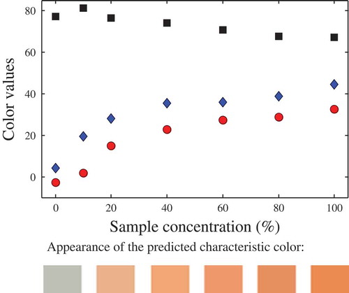
Figure 5. Characteristic colour of the blue energy drink, at different concentrations. Symbols: (

) L*; (

) a*; (

) b*. Patches with the predicted RGB colours are shown.

In addition, the effect of the background colour was evaluated using the blue energy drink sample. As it can be seen in Fig. 6, the three colour parameters tend to similar values as the depth increases, independent of the background colour. Eq. (1) was fitted for each individual pixel of the 20 patches, using 10 × 10 pixels in each patch, and thus 100 fitting procedures were performed for each curve. To complete this analysis in a statistical way, Table 3 details the average values and the standard deviations of the characteristic colour predicted with the different backgrounds. At first, very similar values were obtained. However, the hypothesis test on the mean equality concluded that the influence of the background was significant because of the very low standard deviations of the measurements.

Table 3. Characteristic colour predicted using different background, for cool blue energy drink sample.

	Background colour
	Yellow	Green	White	Black
L*	55.89 ± 0.21^a	54.63 ± 0.26^b	55.86 ± 1.23^a	56.77 ± 1.43^c
a*	−41.54 ± 0.34^a	−39.74 ± 0.26^b	−41.29 ± 0.33^c	−39.86 ± 1.05^b
b*	−27.03 ± 0.29^a	−27.17 ± 0.96^a	−26.83 ± 0.73^b	−27.49 ± 0.82^c

Same letter in the same row indicates no significant differences (confidence level α = 0.05).

Figure 6. Effect of the background colour on liquid colour prediction. a) L*; b) a*; c) b*. Background colour: (

) yellow; (

) green; (

) white; (

) black. Dashed line represents Eq. (1) fitting.

Again, the L*a*b* colour values of the blue energy drink, measured with different backgrounds, were transformed to RGB values. These results are shown in Fig. 7. From this figure, it is evident that colour differences are notorious at small depths, and then the colour seems to remain constant. In this sense, Fig. 8 shows the total colour difference ΔE (calculated with Eq. (3) assuming the initial colour value for each background as the reference) versus the cell depth z. This relationship was accurately fitted to an exponential equation:

(6)

Figure 7. Predicted colour variation with depth for the blue energy drink sample, using different background colours.

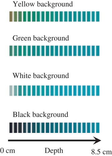
Figure 8. Total colour difference ΔE versus depth for different background colours: (

) yellow; (

) green; (

) white; (

) black. Dashed line represents Eq. (6) fitting.

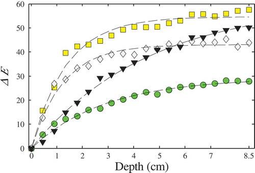
From this equation, a characteristic depth z, required to achieve a desired total colour difference, is defined:

(7)

For instance, from Eq. (7) the cell depth required to obtain 50% of variation on the total colour difference () for red and white wine was 4.5 and 37.2 mm, respectively. Hernández et al.^[8] estimated an average thickness of 3.6 mm of wine when measuring colour on the rim of a sample holder. It is important to mention that for less translucent samples, the cell does not need be full filled, or small cells can be used. On the contrary, for more translucent samples, a higher depth could be necessary. Finally, in addition to predict the characteristic colour, defined as the value predicted at infinite depth, the proposed methodology could be used to obtain the colour at an arbitrary depth, using a desired background.

Conclusion

In this work, a novel methodology to measure and characterise the colour of translucent liquid foods was proposed. Typically, this property is measured using spectrophotometers. However, with this methodology, the obtained colour does not resemble the colour as it is perceived by the consumers. The colour of the liquid samples was measured using digital images, and the characteristic colour was defined as the colour at infinite depth. A cell with a tilted floor was designed and built ad hoc, so that different depths could be evaluated simultaneously in a single image. An empirical mathematical conversion between RGB and CIELAB colour spaces was employed, as well as a standard colour chart for calibration purposes. The experimental results of colour versus depth were fitted to an exponential equation, from which the characteristic L*_∞, a*_∞, and b*_∞ colour values were obtained. The proposed methodology allowed obtaining a successful colour prediction. Also, the total colour difference ΔE versus the cell depth was accurately fitted to an exponential equation, thus defining a characteristic depth, an important parameter in the design of measurement cells for specific liquid foods. In general, colour predictions obtained from the image processing methodology better resemble the food samples in a visual sense, and for most samples, a high correlation between image analysis and spectrophotometer Hue values was obtained.

References

- Pathare, P.B.; Opara, U.L.; Al-Julanda Al-Said, F. Color Measurement and Analysis in Fresh and Processed Foods: A Review. Food and Bioprocess Technology 2013, 6(1), 36–60.
- Wu, D.; Sun, D.-W. Color Measurements by Computer Vision for Food Quality Control - A Review. Trends in Food Science and Technology 2013, 29(1), 5–20.
- CIE DS 014-4.3/E. Colorimetry - Part 4: CIE 1976 L*A*B* Color Space. Commission Internationale De L’eclairage, 2007. Central Bureau: Vienna, Austria, 2007.
- McCaig, T.N. Extending the Use of Visible/Near-Infrared Reflectance Spectrophotometers to Measure Color of Food and Agricultural Products. Food Research International 2002, 35(8), 731–736.
- Joubert, E. Tristimulus Color Measurement of Rooibos Tea Extracts as an Objective Quality Parameter. International Journal of Food Science and Technology 1995, 30(6), 783–792.
- Huertas, R.; Melgosa, M.; Negueruela, A.I. Color Coordinates of Wine Samples with Different Thicknesses. Color Research and Application 2005, 30(2), 149–152.
- González-Miret Martín, M.L.; Ji, W.; Luo, R.; Hutchings, J.; Heredia, F.J. Measuring Color Appearance of Red Wines. Food Quality and Preference 2007, 18(6), 862–871.
- Hernández, B.; Sáenz, C.; De La Hoz, J.H.; Alberdi, C.; Alfonso, S.; Diñeiro, J.M. Assessing the Color of Red Wine like a Taster’s Eye. Color Research and Application 2009, 34(2), 153–162.
- Gómez-Robledo, L.; Melgosa, M.; Huertas, R.; Roa, R.; Moyano, M.J.; Heredia, F.J. Virgin-Olive-Oil Color in Relation to Sample Thickness and the Measurement Method. Journal of the American Oil Chemists’ Society 2008, 85(11), 1063–1071.
- Carvalho, M.J.; Pereira, V.; Pereira, A.C.; Pinto, J.L.; Marques, J.C. Evaluation of Wine Color under Accelerated and Oak-Cask Ageing Using Cielab and Chemometric Approaches. Food and Bioprocess Technology 2015, 8(11), 2309–2318.
- Iqbal, S.M.D.; Gopal, A.; Sankaranarayanan, P.E.; Nair, A.B. Classification of Selected Citrus Fruits Based on Color Using Machine Vision System. International Journal of Food Properties 2016, 19(2), 272–288.
- Fernández-Vázquez, R.; Stinco, C.M.; Hernanz, D.; Heredia, F.J.; Vicario, I.M. Color Training and Color Differences Thresholds in Orange Juice. Food Quality and Preference 2013, 30(2), 320–327.
- Mendoza, F.A.; Kelly, J.D.; Cichy, K. Automated Prediction of Sensory Scores for Color and Appearance in Canned Black Beans (Phaseolus Vulgaris L.) Using Machine Vision. International Journal of Food Properties 2017, 20(1), 83–99.
- Atkins, P.; De Paula, J. Atkins’ Physical Chemistry, 8th edn.; WH Freeman and Company: New York, 2006.
- Yang, L.; Kruse, B. Revised Kubelka-Munk Theory. I. Theory and Application. Journal of the Optical Society of America A 2004, 21(10), 1933–1941.
- Goñi, S.M.; Salvadori, V.O. CIELAB Color Measurement from Digital Images. Servicio De Difusión De La Creación Intelectual, Repositorio Institucional De La UNLP. http://hdl.handle.net/10915/45660, 2015.
- Goñi, S.M.; Olivera, D.F.; Salvadori, V.O. Determinación De Color En El Espacio CIELAB a Partír De Imágenes Digitales. In: Conference on Food Innovation FoodInnova 2014, Concordia, Entre Ríos, Argentina, 20–23 October 2014, Vol. 2 pp. 538–546, 2016.
- Goñi, S.M.; Salvadori, V.O. Color Measurement: Comparison of Colorimeter versus Computer Vision System. Journal of Food Measurement and Characterization 2017, in press, doi: 10.1007/s11694-016-9421-1
- IEC 61966-2-1. Color Measurement and Management in Multimedia Systems and Equipment – Part 2-1: Default RGB Color Space – sRGB. International Electrotechnical Commission, Geneva, Switzerland, 1999.
- Gonzalez, R.C.; Woods, R.E. Digital Image Processing, 2nd.; Prentice Hall: New Jersey, 2002.
- León, K.; Merry, D.; Pedreschi, F.; León, J. Color Measurement in L*A*B* Units from RGB Digital Images. Food Research International 2006, 39(10), 1084–1091.
- Lee, D.-J.; Archibald, J.K.; Chang, Y.-C.; Greco, C.R. Robust Color Space Conversion and Color Distribution Analysis Techniques for Date Maturity Evaluation. Journal of Food Engineering 2008, 88(3), 364–372.
- Valous, N.A.; Mendoza, F.; Sun, D.-W.; Allen, P. Color Calibration of a Laboratory Computer Vision System for Quality Evaluation of Pre-Sliced Hams. Meat Science 2009, 81(1), 132–141.
- Quevedo, R.A.; Aguilera, J.M.; Pedreschi, F. Color of Salmon Fillets by Computer Vision and Sensory Panel. Food and Bioprocess Technology 2010, 3(5), 637–643.
- Jackman, P.; Sun, D.-W.; ElMasry, G. Robust Color Calibration of an Imaging System Using a Color Space Transform and Advanced Regression Modeling. Meat Science 2012, 91(4), 402–407.
- Salmerón, J.F.; Gómez-Robledo, L.; Carvajal, M.Á.; Huertas, R.; Moyano, M.J.; Gordillo, B.; Palma, A.J.; Heredia, F.J.; Melgosa, M. Measuring the Color of Virgin Olive Oils in a New Color Scale Using a Low-Cost Portable Electronic Device. Journal of Food Engineering 2012, 111(2), 247–254.
- Girolami, A.; Napolitano, F.; Faraone, D.; Braghieri, A. Measurement of Meat Color Using a Computer Vision System. Meat Science 2013, 93(1), 111–118.
- Pascale, D.; RGB Coordinates of the Macbeth Colorchecker. Available at: http://www.babelcolor.com/download/RGB/Coordinates of the Macbeth ColorChecker.pdf, 2006. (Last accessed Aug 18 2016).
- CIE 15. Colorimetry. 3rd Edn. Technical Report CIE 15:2004, Commission Internationale de l’Eclairage, 2004.
- Ohno, Y. Chapter 5: Spectral Color Measurement. Colorimetry: Understanding the CIE System, Schanda, J.; Eds.; Wiley: New York; 2007.
- Hines, W.W.; Montgomery, D.C. Probability and Statistics in Engineering and Management Sciences, 3rd edn.; John Wiley & Sons, Inc.: USA, 1990.
- Goñi, S.M.; Salvadori, V.O. Predicción Del Color De Líquidos En El Espacio CIELAB a Partir De Imágenes Digitales. In: INNOVA 2015, 7º Simposio Internacional de Innovación y Desarrollo de Alimentos, 10º Congreso Iberoamericano de Ingeniería de Alimentos, Montevideo, Uruguay, 7–9 October 2015.