Simulation of gaseous pollutant dispersion around an isolated building using the k–ω SST (shear stress transport) turbulence model

ABSTRACT

The dispersion of gaseous pollutant around buildings is complex due to complex turbulence features such as flow detachment and zones of high shear. Computational fluid dynamics (CFD) models are one of the most promising tools to describe the pollutant distribution in the near field of buildings. Reynolds-averaged Navier-Stokes (RANS) models are the most commonly used CFD techniques to address turbulence transport of the pollutant. This research work studies the use of closure model for the gas dispersion around a building by fully resolving the viscous sublayer for the first time. The performance of standard model is also included for comparison, along with results of an extensively validated Gaussian dispersion model, the U.S. Environmental Protection Agency (EPA) AERMOD (American Meteorological Society/U.S. Environmental Protection Agency Regulatory Model). This study’s CFD models apply the standard and the turbulence models to obtain wind flow field. A passive concentration transport equation is then calculated based on the resolved flow field to simulate the distribution of pollutant concentrations. The resultant simulation of both wind flow and concentration fields are validated rigorously by extensive data using multiple validation metrics. The wind flow field can be acceptably modeled by the model. However, the model fails to simulate the gas dispersion. The model outperforms in both flow and dispersion simulations, with higher hit rates for dimensionless velocity components and higher “factor of 2” of observations (FAC2) for normalized concentration. All these validation metrics of model pass the quality assurance criteria recommended by The Association of German Engineers (Verein Deutscher Ingenieure, VDI) guideline. Furthermore, these metrics are better than or the same as those in the literature. Comparison between the performances of and AERMOD shows that the CFD simulation is superior to Gaussian-type model for pollutant dispersion in the near wake of obstacles. AERMOD can perform as a screening tool for near-field gas dispersion due to its expeditious calculation and the ability to handle complicated cases. The utilization of to simulate gaseous pollutant dispersion around an isolated building is appropriate and is expected to be suitable for complex urban environment.

Implications: Multiple validation metrics of turbulence model in CFD quantitatively indicated that this turbulence model was appropriate for the simulation of gas dispersion around buildings. CFD is, therefore, an attractive alternative to wind tunnel for modeling gas dispersion in urban environment due to its excellent performance, and lower cost.

Introduction

With growing worldwide urbanization, the quantification of wind flow field and gaseous pollutant dispersion around buildings is of great environmental, health, and safety significance. This information is necessary for authorities to achieve the objectives of local air quality management (Mumovic et al., 2006), and it also ensures the design of a comfortable and healthy built environment (Ai and Mak, 2013). In addition, the information assists risk analysis and emergency response decision in the accidental release of toxic and/or flammable gases (Pontiggia et al., 2011; Labovský and Jelemenský, 2013).

However, the accurate prediction of air pollutant dispersion within urban canopy layer is complicated largely by the interaction between atmospheric flow and flow around buildings (Schatzmann et al., 2010). Gaussian-type dispersion models, including AERMOD (American Meteorological Society/U.S. Environmental Protection Agency Regulatory Model) and California Puff Model (CALPUFF), have been successfully used to simulate emissions from large elevated sources such as power plant stacks and are recommended by global regulatory agencies for environmental assessments (Lakes Environmental Research Inc., 2016). These models include the effect of buildings on dispersion within a surface roughness instead of resolving fluid dynamic equations explicitly. For example, the plume behavior in the wake of a building is represented as a close approximation by the Plume Rise Model Enhancements (PRIME) algorithm in AERMOD and CALPUFF (Melo et al., 2012). The PRIME algorithm accounts for enhanced plume dispersion caused by the turbulent wake of the building, as well as for reduced plume rise owing to descending streamlines and increased entrainment in the wake (Petersen and Guerra, 2016). It explicitly computes the fields of wind velocity, turbulent intensity, and streamline slope as a function of building geometry within the wake of the building (Schulman et al., 2000). The plume rise trajectory is then numerically solved, taking stack location, streamline deflection near the building, vertical wind speed shear, and velocity deficit into account (Cimorelli et al., 2004). Gaussian plume and puff models can model different cases expeditiously and are very suitable for pollutant dispersion in the far field of obstacles.

Computational fluid dynamics (CFD)-based microscale meteorological models have become an emerging and promising tool for pollutant dispersion in an urban environment. Such a CFD simulation usually entails solving Navier–Stokes equations coupled with either a passive concentration transport equation or a particle tracking algorithm (Gorlé et al., 2010a). Approaches used to numerically solve turbulent flow equations in previous studies include Reynolds-averaged Navier–Stokes (RANS) method, large eddy simulation (LES), and detached eddy simulation (DES). RANS method is most commonly utilized due to balance between accuracy and computational effort. It requires a closure turbulence model such as and for Reynolds stresses (Moukalled et al., 2015). LES, where larger turbulence scales are resolved, is inherently more accurate than RANS at the expense of greater computational requirements (Gorlé et al., 2010a). A DES combines LES in the separated regions and RANS mode in the boundary layers (Kakosimos and Assael, 2013). The acceptance of microscale meteorological models has been promoted with the advancement in computer science.

Great effort has been put into the CFD-based microscale air dispersion modeling. The majority of previous studies used standard closure model and its variants for near-field pollutant dispersion around buildings. Although LES and DES models have already been used for large-scale projects, few researchers utilized LES and DES models for near-field simulation. To our best knowledge, we employ the turbulence model with fully resolved viscous sublayer to simulate gas flow and dispersion under outdoor urban environment in CFD for the first time in the current work, and we validate the simulation with extensive wind tunnel data quantitatively. The validation metrics, including hit rate, “factor of 2” of observations (FAC2), and fractional bias (FB), are adopted for quality assurance. The advantage of model is manifested by comparison with available results in the literature. AERMOD’s the wake of a building is also included for comparison.

Literature review

Previous studies on CFD-based air dispersion modeling are briefly summarized. Mavroidis et al. (2007) compared atmospheric dispersion around a cubic building between standard (SKE) model and one-equation model in the code ADREA-HF. Both turbulence models provided satisfactory performance, with a ratio of calculated to experimental value between 1.1 and 2.0 for most sampling points. However, these models failed to simulate wake concentrations; they overestimated the concentration by a factor of 4.5–5.0 in the recirculation region. Tominaga and Stathopoulos (2009) compared the performance between different types of model for the dispersion around a cubic building in a self-developed code. They concluded that SKE was inappropriate for the simulation of concentration field because it could not produce basic flow structure, whereas revised models performed better than SKE. However, all models produced poor predictions for concentration distribution at the side and leeward surface of the building. They later slightly improved the simulation performance using LES (Tominaga and Stathopoulos, 2010). The same authors also simulated pollutant dispersion around building array using RNG (Re-Normalisation Group) model and LES and demonstrated that LES gave better results. Gorlé et al. (2010b) studied the gas dispersion in the wake of a rectangular using two RANS modeling approaches in Fluent version 6.3. The closure turbulence models were standard model and its Kato–Launder (KL) variant. The hit rates (q) of longitudinal velocity component (u) and nondimensional concentration K were 0.66–0.71 and 0.58–0.76, respectively. Interestingly, the best simulation in flow field in the above work produced the worst simulation for the concentration field.

Chavez et al. (2011) applied realizable model in Fluent to study the gas dispersion in three building environments and pointed out the importance of turbulent Schmidt number (Sc_t) in CFD modeling. The Sc_t number correlates the eddy diffusivity (D_t) for pollutant transport in turbulent flow with turbulence viscosity (). Cheng and Liu (2011) used LES method coupled with one-equation subgrid-scale (SGS) parametrization to simulate pollutant dispersion in two-dimensional (2D) street canyons in OpenFOAM 1.5. Their LES results on concentration transport qualitatively agreed with most experimental and simulation data in the literature, but the work did not provide quantitative analysis. Huang et al. studied the effects of upstream building on the wind flow and pollutant dispersion within an isolated street canyon (Huang et al., 2014) and multiple-block street canyon (Huang et al., 2015) using the k – ε based models in Fluent. Their simulation results were validated by wind tunnel data satisfactorily before further sensitivity analysis. Kakosimos and Assael (2013) applied DES in ProMTGD software to microscale pollution dispersion by combining the advantages of LES and RANS. The DES results were validated well by 966 data points of Case A1-5 on CEDVAL database (CEDVAL, 2006). Interested readers can refer to available review articles (Tominaga and Stathopoulos, 2013; Lateb et al., 2016) for additional information.

Most researchers used RANS technique coupled with standard or modified turbulence models in pollutant dispersion around buildings. Nevertheless, several professional guidelines stated that model should not be used in the wind environment prediction because standard model cannot predict the reverse flow on the building roof, whereas revised linear failed to predict the flow field in the wake region (Shao et al., 2012). Fewer investigators utilized LES or DES methods. However, closure turbulence models received much less attention, although it can be integrated all the way to the wall (Wilcox, 2004). Perhaps the sensitivity to free stream of Wilcox’s original model restricted its utilization. The shear stress transport (SST) model resolved this issue by combining respective strength of and models via a blending function (Menter, 1993, 1994).

The SST model uses model inside the boundary layer, and model in the free shear flow. Its main feature is the improved performance in adverse pressure gradients and separating flows (Moukalled et al., 2015). Moreover, its advanced wall treatment allows the model to fully resolve the boundary layer at a y⁺ value of approximately 1, thereby capturing detailed information in the wall regions (Menter et al., 2003a). As a result, it is an excellent platform for the application of DES (Menter, 2009). Despite the aforementioned advantages, the model has been rarely utilized in the air dispersion modeling under urban environment. King et al. (2015) studied the wind flow and pollutant dispersion within urban street canyon using k–ω SST model. They utilized a wall function for the boundary layer. However, they only validated their flow simulation graphically. Furthermore, the k–ω SST model has already been employed to simulate wind flow within built environment and airflow of the cross-ventilation of a building. Rakai and Kristóf attempted to use k–ω SST model to simulate the flow field of a mock urban setting but did not achieve satisfactory simulation results (Rakai and Kristóf, 2010). Blocken’s group concluded that k–ω SST model outperformed its k–ε based counterparts in the flow simulation of building cross-ventilation (Ramponi and Blocken, 2012; Perén et al., 2015). These three works only reported the flow modeling and again used wall functions for wall treatment. Furthermore, the model has been widely accepted in the wind energy industry to assess the aerodynamic performance of turbine airfoils, where the modeling domain is on the order of dozens of meters (Campobasso et al., 2013; Rocha et al., 2014, 2016). Unlike flow simulations mentioned above, the advanced wall treatment that fully resolved the viscous sublayer was highly recommended in wind turbine simulation (Maître et al., 2013). The wall regions are of special interest in the dispersion modeling because the outdoor pollutants in these areas can enter the indoor environment through ventilation. This phenomenon is termed as exhaust cross-contamination, and it causes health problem to the building dwellers (Chávez, 2014). Therefore, fully resolving the viscous sublayer is preferred in the near-field dispersion modeling.

The pollutant dispersion under urban environment includes both flow and dispersion simulation. An accurate flow simulation is a prerequisite rather than a guarantee of a reliable dispersion modeling (Gorlé, 2009). Previous studies using k–ω SST model focused primarily on flow simulation and used wall functions for viscous boundary sublayer. Now that the k–ω SST outweighs the RANS k–ε models in the flow simulation, it is, thus, expected to behave well in the dispersion modeling. Given the limited number of reporting k–ω SST model in the dispersion modeling under urban environment, it is reasonable to study its feasibility starting from the simplest geometry before application to more complex configuration. The extensive studies on the dispersion around an isolated building using k–ε models in the literature support this methodology. This research study employs the , which is more computationally intensive, but one would expect it to be more suitable for the near-field gas dispersion simulation than the model adopted in previous studies. More importantly, we take advantage of the advanced wall treatment in the k–ω SST model to integrate all the way to the wall instead of using wall functions. Furthermore, a damping coefficient in the turbulent viscosity can be added to for transitional flows at low Reynolds number if necessary (Wilcox, 1994; ANSYS Inc., 2013).

It is also observed that proprietary software packages, such as ANSYS Fluent, are widely used in the literature (Zhang et al., 2015). Recently, open source software, such as OpenFOAM, has attracted more attention in the CFD community (Franke et al., 2012; Flores et al., 2013). Advantages of open source CFD codes over proprietary software packages include the access to source code and the development of customized solvers. Efficient pre- and postprocessing tools such as parallel simulation and mesh generation and manipulation utilities make OpenFOAM attractive to users (Liu et al., 2016).

Validation is another important part of microscale CFD dispersion modeling that deserves special attention (Lateb et al., 2016). Most studies reviewed above validated their CFD models by qualitative comparison between experimental and predicted values. To resolve this issue, several quantitative validation metrics have been developed to evaluate the CFD simulations (Schatzmann et al., 2010). Among them, hit rate is the accepted metric for vector velocity (Franke et al., 2012), “factor of 2” of observations (FAC2), and fractional bias (FB) are the recommended statistics for scalar concentration by Kakosimos and Assael (2013). There are also comprehensive wind tunnel data sets available online for rigorous validation purpose, for example, the well-known CEDVAL Web site maintained by Hamburg University (CEDVAL, 2006). The CEDVAL A1-5 is frequently used in the literature for the validation of gas dispersion around buildings (Gorlé et al., 2010b; Ai and Mak, 2013; Kakosimos and Assael, 2013).

In this paper, gaseous pollutant dispersion around a rectangular building is simulated by our customized solver, concenSimpleFoam, based on the built-in simpleFoam in OpenFOAM 2.3.1 package. The Navier-Stokes equations are numerically solved by standard or . The concentration field around the building is computed by solving a passive chemical concentration transport based on the resolved flow field. Simulated wind flow field and concentration field are then validated by extensive wind tunnel data points. There are more than 1000 data points for normalized velocity and for concentration calculations. Finally, the performance of SST model is compared with that of AERMOD model, model, and other numerical techniques in the literature.

SST turbulence model

The SST turbulence model is a two-equation eddy-viscosity model. The prognostic equations of turbulent kinetic energy () and specific dissipation rate () for steady-state incompressible flow are described in eqs 1 and 2 (Menter et al., 2003b; OpenCFD Ltd., 2015).

(1)

(2)

where u_i is the mean velocity in the x_i direction in which i = 1, 2, and 3 represent the x, y, and z directions, respectively. is the flow density, and and are the molecular and turbulent viscosity of the flow, respectively. P_k is the production of turbulence energy, and a production limiter to prevent turbulence buildup in stagnation regions. Turbulence production terms are expressed in the following equations.

(3)

(4)

The blending function, F₁, in eq 2 depends on solution variables and the distance to the nearest wall (y). It is defined by

(5)

with . F₁ equals to zero away from the surface and switches over to unity inside the boundary layer. The blend of and models is achieved through the following schemes, thereby taking advantage of the strengths of both turbulence models.

(6)

(7)

The definition of turbulent viscosity is different from the original model and is expressed in eq 8.

(8)

where S is the invariant measure of the strain rate and F₂ is the second blending function. These two variables are defined by

(9)

(10)

(11)

All constants involved in the SST model are summarized in Table 1. The steady-state flow equations in SST model can be numerically solved using Semi-Implicit Method for Pressure Linked Equations (SIMPLE) algorithm, and the corresponding solver in OpenFOAM is simpleFoam.

Table 1. Constants used in SST model.

Constant
Value	0.85	1.0	0.5	0.856	0.075	0.0828	0.09	5/9	0.44	0.31	1.0

Passive gas concentration transport in turbulent wind flow

The transport equation for scalar concentration can be calculated based on the resolved wind flow field. The general time-averaged governing equation for the concentration transport in an incompressible turbulent flow is given by

(12)

where c is the pollutant concentration, S_c the source term, and D_eff the effective diffusivity in a turbulent flow, which is the sum of molecular diffusivity (D) and eddy diffusivity (D_t). The eddy diffusivity is defined by

(13)

where Sc_t is called turbulent Schmidt number. The Sc_t is an adjustment factor in the steady RANS simulations, and its optimum value widely ranged from 0.2 to 1.3 in published literature (Tominaga and Stathopoulos, 2007). It is an adjustable parameter in our customized solver in the current study, and it ranges from 0.2 to 1.0. For passive concentration transport, eq 12 is further simplified into

(14)

To resolve all partial differential equations, this study developed a customized solver, concenSimpleFoam, based on the built-in simpleFoam solver in OpenFOAM.

Modeling strategies

Test case

In the present work, comprehensive CEDVAL experimental data collected in a high-quality standard are used to verify the pollutant dispersion simulation using SST turbulence model in OpenFOAM. The experiments were performed at a scale of 1:200 in the Blasius wind tunnel at the University of Hamburg (CEDVAL, 2006). The atmospheric stability in wind tunnel was neutral. Figure 1 shows the geometry of the rectangular model building, whose height H = 125 mm, length L = 100 mm, and width W = 150 mm. Four tracer gas sources were located close to the ground on the leeward wall representing emissions from an underground parking garage. Figure 1 shows at the bottom right corner a zoomed-in view on one of the four sources. The inflow wind direction is 270° (west). Wind flow around the rectangular building was measured by laser Doppler velocimetry (LDV) within two sample planes: y = 0 (603 points) and z = 0.035 m (643 points). Corresponding results were presented in Case A1-1 on the CEDVAL Web site. The results of gas dispersion around the same building were published in Case A1-5 of the CEDVAL database. There were 1228 data points collected by flame ionization detector (FID) on six sample planes, including x = 51 mm, y = 0, y = −60 mm, y = −76 mm, z = 10 mm, and z = 35 mm. These measurement planes cover almost all regions of interest in the near-field pollutant dispersion modeling. It is noted that the measured concentrations were presented in a dimensionless form as follows.

(15)

Figure 1. Schematic view of the CEDVAL Case A1-5 building geometry.

where and are the measured tracer gas concentration and tracer gas concentration at the sources. is the reference wind speed measured at the reference height of 0.66 m. is emission rate of tracer gas at the sources.

Numerical techniques in CFD

The computational domain is constructed according to both AIJ (Architectural Institute of Japan) and COST (European Cooperation in Science and Technology) guidelines (Franke, 2006; Tominaga et al., 2008b). The inflow boundary is located 7.6H upwind of the building, and outflow boundary is set at 10H behind the building. The lateral and the top boundary are all located 5H away from the building. Figure 2 illustrates more details of the computational domain. The computational domain and a base level mesh density are first defined by constructed hexahedral meshes generated by blockMesh utility. Then the background meshes are refined by the built-in snappyHexMesh utility for the simulation of pollutant dispersion. In this work, both standard and SST models are utilized.

Figure 2. Illustration of the computational domain.

The meshing strategy differs between each turbulence model. Standard model requires wall functions to avoid the resolution of near-wall boundary layer. The wall adjacent cells are expected to be located in the logarithmic layer to ensure the accuracy of simulation. Therefore, the value of normalized distance to the wall (y⁺) is expected to be between 30 and 300 (Kalitzin et al., 2005). However, SST model has more advanced near-wall treatment, and can automatically shift between low Reynolds correlations and wall functions (Menter et al., 2003a). In order to simulate near-field pollutant dispersion, a y⁺ value smaller than 2 is desired. This work analyzed optimal grid cell numbers and spacing, arriving at approximately 1.17 million cells (including 1.16 million hexahedra) for the model. The maximum aspect ratio is 1.022; minimum and maximum cell volumes are 3.86 × 10⁻⁸ and 2.47 × 10⁻⁶ m³, respectively. The average nonorthogonality is 2.08. The average y⁺ values for ground and building patches are 134.3 and 31.5, respectively. As for SST model, our analysis required 1.44 million cells (including 1.41 million hexahedra), with average y⁺ values of 0.54 and 1.78 for ground and building patches, respectively. The maximum aspect ratio is 91.6; minimum and maximum cell volumes are 1.07 × 10⁻¹² and 5.13 × 10⁻⁵ m³, respectively. The average nonorthogonality is 4.04. Further refinement of meshes will not improve the simulation performance, when compared with experimental results.

Proper boundary and initial conditions are needed for all patches to run the simulation. They are summarized in Table 2, where c is the concentration, I the turbulence intensity that is assumed to be 10%, l the mixing length, p the pressure, u the wind velocity, the friction velocity calculated from the reference velocity, z the elevation, z₀ the surface roughness length, and the von Karman’s constant. It is noted that the velocity profile, , and at inlet are given for atmospheric boundary layer (ABL) flow (Richards and Hoxey, 1993). Minor modifications to wall treatment and top boundary condition suggested by Hargreaves and Wright (2007) are also accepted in the simulation. As for model, by definition, in which . Most previous studies used based models; therefore, the effectiveness of using ABL boundary condition is examined by passing a wind flow throughout the computational domain without buildings (Mochida et al., 2002). The vertical profiles of velocity and at inlet should be maintained to the outlet boundary in this test if ABL conditions are applicable.

Table 2. Boundary conditions utilized in and turbulence models.

Boundary/patch
Inlet
Outlet	Zero gradient for and ; Zero for pressure	Zero gradient for and ; Zero for pressure
Ground, building	Standard wall function for k and ;	Zero gradient for c and p;
	Zero gradient for c and p;	Zero for and u;
	Zero for u
Tracer gas source	; ;	; ;
	Zero gradient for p;	Zero gradient for p;
	;	;
Top, front, and back	Slip	Slip

The current work developed a customized solver based on built-in simpleFoam solver to incorporate the passive concentration transport equation. The SIMPLE algorithm numerically resolves the coupling between pressure and velocity fields in the RANS equations. The discretization schemes are selected according to the balance of simulation accuracy and stability. The least squares and Gauss linear limited schemes are used for gradient and Laplacian terms, respectively. The Gauss linear upwind scheme coupled with gradient limiters is utilized for the divergence terms of velocity, k and . Its truncation error is + …, where denotes the distance between the upwind and far upwind nodes of the particular face, indicating a second-order accuracy (Moukalled et al., 2015). Gamma differencing scheme is employed for the divergence term of concentration to avoid nonphysical values. The Gamma differencing scheme is a blend between first-order upwind differencing (UD) and second-order central differencing (CD). It is deemed as a bounded version of second-order CD. It ensures boundedness by a local normalized indicator, . The CD is utilized wherever the boundedness requirements are satisfied (e.g., ); otherwise, the UD is employed (Jasak et al., 1999). The generalized geometric-algebraic multigrid (GAMG) solver is used for pressure, and the smoothSolver for others. The convergence criteria for variables are 10⁻⁴, except 10⁻³ for pressure and velocity in the y direction, and 10⁻⁶ for concentration. Such criteria are tighter than that used in previous study (Franke et al., 2012). All simulations are then processed in parallel using Linux servers.

The metrics recommended by the COST guideline are accepted in this work to validate the use of turbulence model in CFD for the simulation of gaseous pollutant dispersion (Schatzmann et al., 2010; Franke et al., 2012; Kakosimos and Assael, 2013). The vector velocity components are quantitatively analyzed using hit rate, whereas scalar concentration is validated by FAC2, FB, and geometric mean bias (MG). The expression of hit rate is presented as follows.

(16)

with

(17)

where q is the hit rate, and n is the total number of effective measurements. P_i and E_i are the predicted value of CFD and experimental value, respectively, at location i. is the relative uncertainty of the comparison data. It is the sum of the reproducibility of wind tunnel measurements and the allowed inaccuracy of the simulation results. It equals 0.25 for the current case (The Association of German Engineers [Verein Deutscher Ingenieure, VDI], 2000). is the allowable absolute deviation, which represents the repeatability of the comparison data and the uncertainty introduced through interpolation. A value ranging from 0.060 to 0.083 was reported in the literature (VDI, 2005; Gorlé et al., 2010b; Franke et al., 2012; Kakosimos and Assael, 2013) for the current case. In this study, the minimum is accepted to ensure rigorous validation.

FAC2 describes the fraction of CFD predictions that fall within a factor of 2 of the experimental observations. It is similar to hit rate, and defined as

(18)

with

(19)

FB reveals systematic errors by measuring the mean bias linearly and is described in the following equation. This metric is not appropriate for a vector such as velocity.

(20)

where and denote the average of experimental and predicted values, respectively. Different from FB, MG shows the mean bias logarithmically, as described in eq 21.

(21)

with

(22)

Normalized velocity and concentration are used in the validation. The acceptable criteria to pass the validation are , and (VDI, 2005; Schatzmann et al., 2010).

AERMOD simulation

The AERMOD simulation employs the full scale of the test case described in the section “Test case.” The data input used Lakes Environmental Research Inc.’s AERMOD View (Lakes Environmental Research Inc., 2015). Appropriate scaling rules should be applied to ensure wind tunnel simulations can represent field experiments (Mavroidis et al., 2003). The dominant dimensionless groups are boundary layer parameter, , and time scale factor U_t/H at Reynolds numbers beyond 11000, in which is the averaging time (Aubrun and Leitl, 2004). Schatzmann and Leitl (2002) experimentally observed that the agreement between field and wind tunnel data was satisfactory using these two factors. Melo et al. (2012) also accepted these two dimensionless parameters for the simulation of odor dispersion near a pig barn. Therefore, such dimensionless parameters are used for scaling in the current work. As mentioned above, the geometry scale ratio is 1:200, and the atmosphere is neutrally stable. The input parameters of AERMOD are then summarized as follows.

Theoretically, the Monin-Obukhov length (L) is infinite for neutral atmospheric stability (Cimorelli et al., 2004). In this work, a sufficiently large number, L = 500000 m, is used according to Bonifacio et al. (2014). The sensible heat flux, surface friction velocity, and convective and mechanical mixing heights are calculated using formulations from AERMOD (Cimorelli et al., 2004) with Bowen ratio and albedo equal to 2.0 and 0.2, respectively (Bonifacio et al., 2013).

The effect of buildings on plume dispersion is processed by the U.S. Environmental Protection Agency (EPA) Building Profile Input Program Plume Rise Model Enhancements (BPIP-PRIME) to support building downwash. As BPIP handles point sources only, equivalent point sources with the same area as the four tracer sources are used. Uniform Cartesian receptor grids are utilized to cover the area of interest (X/H = −0.4–3.2 and Y/H = −2.2–0) for sampling height of 2 m.

Results and discussion

Wind profile at inlet

Inlet condition largely affect the simulation of performance. The ABL conditions developed by Richards and Hoxey (1993) for model are examined by passing flow over the computational domain without obstacles. Figure 3 shows the flow conditions at inlet and outlet boundaries of the examination case. The left side presents the vertical velocity profile at both inlet and outlet boundaries, whereas right side illustrates the profiles. The wind tunnel experimental data are also included to show the goodness of ABL condition. It can be seen that experimental data can be well expressed by the ABL condition, with the largest deviation of 6.0%. It is observed that the difference between inlet and outlet velocities is in general within ±5.0% except the lowest vertical positions (around 10% of the wind tunnel experimental height), and the vertical profile can be maintained throughout the computational domain. Similar observations are found for the profile. In principle, the inlet distribution matches with the outlet counterpart well; few relatively large deviations again occur in the lower section of the domain. Therefore, one can conclude that in the current study, the ABL conditions can be used for the simulation of wind flow and gas dispersion using model in the CFD.

Figure 3. Comparison between conditions at inlet and outlet boundaries of model.

Performance of different RANS models

In the present study, standard and models are selected to simulate the gaseous pollutant dispersion around a rectangular building. Figure 4 shows the comparison between experimental data and simulation results of the model. Dimensionless velocity (, , and ) and normalized concentration (K) are utilized. In the velocity validation in Figure 4a–c, points located in the area confined by solid lines are counted as hits. The solid reference lines represent the relative deviation of ±25%, and absolute deviation of ±0.06. The match-up for dimensionless velocities are acceptable; however, the deviation between experimental observations and optimum predicted K values obtained at Sc_t = 0.2 and 0.4 are relatively larger. The validation metrics for corresponding parameters are summarized in Table 3. The hit rates of , , and using are 0.67, 0.75, and 0.89, respectively. The FAC2 of normalized concentration K is 0.45 and 0.38 for Sc_t = 0.2 and 0.4, respectively. The criteria for quality assurance are , , and (VDI, 2005; Schatzmann et al., 2010). Therefore, it is concluded that the simulation of flow field can pass the validation test, whereas the verification of concentration filed failed.

Table 3. Summary of validation metrics of model (quality criteria are presented in the parentheses).

Parameter
Number of data	1246	643	603	1220
Hit rate (≥0.66)	0.67	0.75	0.89	—
FAC2 (≥0.5)	0.83	0.90	0.99	0.45
FB (−0.3–0.3)	—	—	—	−1.03
MG (0.7–1.3)	1.30	1.09	1.00	0.61

Figure 4. Parity plots of (a) , (b) , (c) , (d) K at Sc_t = 0.2, and (e) K at Sc_t = 0.4 for standard model.

Furthermore, Figure 5 shows flow comparison between these two turbulence models at y = 0 plane. Flow over the target building is featured by reattachment on the roof and recirculation in the wake in both simulations. However, the two models produce different length of rooftop reattachment (L_R) and wake circulation (L_W). The definitions of L_R and L_W can be referred to the small sketch on the top left of Figure 5. The values of L_R and L_W are approximately 0.4H and 2.6H, respectively, for standard k–ε model, whereas the counterparts are 0.7H and 1.4H, respectively, for k–ω SST model. The corresponding experimental values are 0.6H and 1.42H (CEDVAL, 2006). It is observed that the k–ω SST model predicts the flow separation better than k–ε model, which has shorter rooftop reattachment length but larger wake recirculation length. Such deviations of k–ε model correspond to Ai and Mak (2013). Figure 6 is another comparison in flow field at z = 0.28H plane. The L_W of the k–ε and k–ω SST models are around 2.1H and 1.6H, respectively. The experimental L_W value is 1.45H. Again, the k–ω SST model outperforms the k–ε model in the prediction of wake recirculation.

Figure 5. Velocity vector plots of k–ε and k–ω SST models at y = 0 plane.

Figure 6. Velocity vector plots of k–ε and k–ω SST models at z = 0.28H plane.

The simulated flow field of the model is close to that reported in a previous study for the same building (Franke et al., 2012). The parity plots in Figure 4 share the same shape as those in the Figure 3 in the reference. Their hit rates for the dimensionless were 0.70, 0.81, and 0.84, respectively, which are close to those summarized in Table 3. The slightly difference could originate from the following areas. First, we used a different wall function from theirs and utilized a larger data set. Furthermore, we accepted a more rigorous absolute deviation value in the validation. Because the focus of this study is not on the model, we present it for comparison purpose. We, thus, did not place extra effort to narrow the difference in the flow field simulation. Franke et al. (2012) did not simulate the concentration field. The reason for the failure of concentration simulation in the current study is probably owing to the intrinsic shortcoming of standard model; this model cannot predict the reverse flow on the building’s roof (Shao et al., 2012). Therefore, we use model in CFD, as it combines the advantages of and models.

Figure 7 shows the simulation of flow and concentration field in comparison with experimental data for model. The CFD model predicted values satisfactorily agree with wind tunnel data. The concentration field is given at Sc_t = 0.2 and 0.4. The validation metrics tabulated in Table 4 further quantitatively confirm that both simulations successfully pass the validation test. When comparing with the results of model, the superiority of model is obvious. All the validation metrics of outperform the counterparts of . The hit rates of , and using model are 0.83, 0.91, and 0.86, respectively, which are greater than corresponding 0.70, 0.81, and 0.84, respectively, using model. As for the simulation of concentration field, the FAC2 of the normalized concentration of is 0.60 and 0.67 at Sc_t = 0.2 and 0.4, respectively. Either is greater than the criterion value of 0.5. Therefore, the dispersion of gaseous pollutant around a building can be successfully simulated by the model. However, the aforementioned analysis shows that model cannot fulfill this purpose. In conclusion, model is a superior numerical tool to standard model in the simulation of gaseous dispersion around a building.

Table 4. Summary of validation metrics of model (quality criteria are presented in the parentheses).

Parameter
Number of data	1230	643	587	1218
Hit rate (≥0.66)	0.83	0.91	0.86	—
FAC2 (≥0.5)	0.94	0.97	0.95	0.60
FB (−0.3–0.3)	—	—	—	−0.08
MG (0.7–1.3)	1.13	1.01	0.95	0.87

Figure 7. Parity plots of (a) , (b) , (c) , (d) K at Sc_t = 0.2, and (e) K at Sc_t = 0.4 for model.

Effect of eddy diffusivity

The eddy diffusivity plays an important role in the gas dispersion around buildings, which is usually much greater than the molecular diffusivity. The eddy diffusivity is correlated with turbulent viscosity through turbulent Schmidt number (Sc_t) as shown in eq 13. 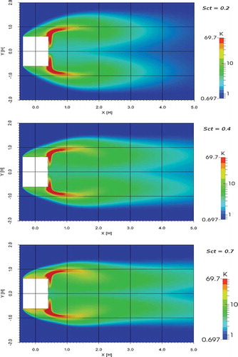Because there is no unified value for the in the passive concentration transport, the effect of Sc_t spanning between 0.2 and 1.0 on concentration simulation of model is studied. Figure 8 shows the concentration field at z = 0.28H plane for Sc_t values between 0.2 and 0.7. As the flow field is independent of Sc_t, it will not be presented. The pollutant lateral dispersion increases and longitudinal transport decreases as the Sc_t value increases. This indicates that a smaller Sc_t value can compensate lateral turbulent diffusion, which corresponds to the comments of Tominaga et al. (2008a).

Figure 8. The concentration distribution for different Sc_t values at z = 0.08H plane.

The validation metrics for different Sc_t values are summarized in Table 5. It can be seen that Sc_t has a significant effect on the simulation performance. A Sc_t value from 0.2 to 0.7 leads to satisfactory performance, as all major validation metrics can meet the quality assurance criteria. The performance of Sc_t = 1.0 is inferior to that of others. Its FAC2 value is lower, and the FB level is slightly beyond the desired range. Sc_t of 0.4 outweighs Sc_t of 0.7 evidently due to better FAC2 and FB values. When comparing the performances of Sc_t values of 0.2 and 0.4, it is observed that Sc_t of 0.2 behaves better in mean bias test (linear and logarithmic), whereas Sc_t of 0.4 better in FAC2 examination. Because FAC2 is the most robust measure about the impact of infrequent occurrence of high or low observations and predictions (Schatzmann et al., 2010), this metric is selected as the preferred if multiple validation metrics meet passing criteria. As a result, a Sc_t of 0.4 is used in the current study to simulate the gaseous pollutant dispersion around a building.

Table 5. Summary of validation metrics at different values (quality criteria are presented in the parentheses).

	Sct
Metric	0.2	0.4	0.7	1.0
FAC2 (≥0.5)	0.60	0.67	0.61	0.54
FB (−0.3–0.3)	−0.08	−0.23	−0.28	−0.32
MG (0.7–1.3)	0.87	0.83	0.85	0.85

It is noted that default Sc_t value in prevalent commercial CFD software is 0.7 (Tominaga and Stathopoulos, 2007). Recent studies showed that reducing the Sc_t value from default 0.7 to approximately 0.4 improved the simulation of concentration field (Di Sabatino et al., 2007; Blocken et al., 2008; Nakiboğlu et al., 2009). Such improvement is probably because the underestimation of turbulent diffusion of momentum often noticed in steady RANS simulation is compensated by the smaller Sc_t value (Tominaga et al., 2008a; Tominaga and Stathopoulos, 2013). Furthermore, the selected Sc_t of 0.4 corresponds well to the estimated value given by an empirical correlation for homogeneous, stationary, and isotropic turbulence (Gorlé et al., 2010b). The estimated value depends on turbulence model constants and spans between 0.42 and 0.54 (Gorlé et al., 2010b). This way, the chosen value in the present study is very close to this range. Therefore, a Sc_t of 0.4 for the current simulation of flow around an isolated building using CFD is appropriate.

Comparison with works in the literature

Three previous studies investigated the gas dispersion around the same building using standard and revised model (Gorlé et al., 2010b; Ai and Mak, 2013) and DES method (Kakosimos and Assael, 2013). Commercial codes were applied in these works. Franke et al. (2012) only reported wind flow simulation using standard for the building. Therefore, these existing literature results are compared with the current work to identify the difference between various studies.

Gorlé et al. (2010b) reported hit rate of dimensionless between 0.66 and 0.7 for various models. Such hit rate is lower than the resulting 0.83 of model in the current study. Their inferior hit rate result is probably again attributable to the inherent shortcoming of model (Shao et al., 2012). The hit rates of and , and FAC2 of dimensionless concentration, K, were not given by Gorlé et al. (2010b). Ai and Mak (2013) placed their emphasis on the effects of inlet conditions and wall treatment on the simulation performance and did not provide quantitative validation metrics data. Kakosimos and Assael (2013) reported detailed validation metrics for the DES simulation. However, the experimental wind flow data set they utilized is different from ours. They used the data of Case C3 of VDI, which was equivalent to Case A1-1 of CEDVAL. Although the same building was used in both cases, the flow data sets were different. There were 1073, 296, and 924 data points for velocity components u, v, and w, respectively, in the work of Kakosimos and Assael (2013). We do not have access to the data of Case C3 of VDI and therefore adopted published flow data of Case A1-1 of CEDVAL (2006). In our work, the number of data points for components u, v, and w is 1230, 643, and 587, respectively. This data set of Case A1-1 of CEDVAL is also accepted by (Franke et al., 2012). Fortunately, Kakosimos and Assael (2013) and we employed the same data set from Case A1-5 of CEDVAL for pollutant dispersion. Yet we used a larger number of points in the validation. The FAC2 and FB values for both studies are almost the same. The FAC2 and FB values are 0.67 and −0.23 for the k–ω SST model using in the current study, and these metrics of the DES are 0.67 and −0.24 in Kakosimos and Assael (2013).

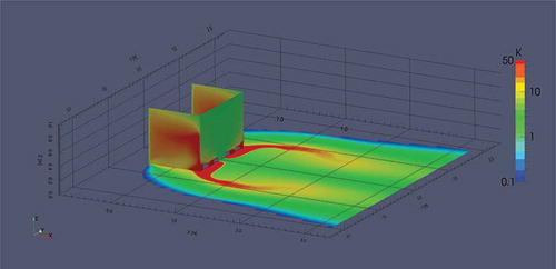
Although the validation metrics of both models over a large number of data points are very close, the pollutant dispersion patterns on building surfaces and ground in the wake are different. Figure 9 illustrates the concentration field on the building walls and on the ground on the side and in the rear of the building. Two major differences have been identified by comparison with that of the DES. Firstly, the longitudinal concentration “overhangs” of the current k–ω SST model are narrower but longer than that of DES. This is probably because the current k–ω SST model is performed at a steady state. It cannot reproduce the flow unsteadiness in the wake region, leading to an underestimated lateral turbulent diffusion (Tominaga and Stathopoulos, 2013). As a result, the longitudinal advection is more dominant. Conversely, DES is an unsteady model and can capture more concentration fluctuations. Therefore, concentrations on the ground located in the building rear are higher due to the enhanced lateral turbulent diffusion. Accordingly, the longitudinal advection is less obvious, leading to a wider and shorter “overhang.” Secondly, the DES produces concentration wiggles whereas the current k–ω SST model does not. This difference is attributable to the averaging of the transient results in the unsteady DES modeling (Kakosimos and Assael, 2013).

Figure 9. The contour plot of dimensionless concentration K on the building and ground.

In summary, model performs better than based models in the literature in the simulation of pollutant dispersion around a building. It delivers equally excellent results in comparison with the DES technique. Therefore, model is a promising technique in the pollutant dispersion in an urban environment.

Comparison with AERMOD model

The utilization of turbulence model for gas dispersion around buildings has been validated rigorously with quantitative validation metrics in sections above. It is of interest to compare the performance between AERMOD and CFD in the pollutant dispersion near buildings. Figure 10 shows the lateral distribution of pollutant concentration at multiple longitudinal distances with between −0.32 and 2.0. The dash line represents AERMOD results, whereas the diamond symbol and solid line describe experimental and CFD data, respectively. As expected, the CFD simulation outperforms AERMOD performance in the representative near wake positions. AERMOD is well-known for its prediction of far-field pollutant dispersion. Melo et al. (2012) showed that AERMOD satisfactorily predicted the odor dispersion downwind a pig barn at = 20, but incorrectly predicted at = 5. The longitudinal distances in Figure 10 are within = 2 because the current objective is to simulate the pollutant dispersion near buildings. Experimental data for far field are not available.

Figure 10. Lateral concentration profiles at different longitudinal positions.

In addition, the longitudinal concentration profiles at various lateral distances are presented in Figure 11. Again AERMOD does not accurately predict gas dispersion in the wake of the target building, whereas CFD simulation can well capture the concentration profile in the area of interest. However, most AERMOD predictions are within 1 order of experimental data. Therefore, Gaussian-type models such as AERMOD can still be used as screening tools in the near-field pollutant dispersion as recommended by COST due to its expeditious calculation and wide application to different complicated dispersion processes (2010).

Figure 11. Longitudinal concentration profiles at different lateral distances.

Limitations and future research

Although this work using steady k–ω SST turbulence model produced nice simulation results validated by extensive wind tunnel data, it can probably be further improved by using the unsteady k–ω SST model, DES or LES approach, as these unsteady methods can better reproduce the flow unsteadiness and concentration fluctuations on the sides and in the wake of buildings (Tominaga et al., 2008a, 2009). Moreover, we will extend the use of k–ω SST turbulence model for pollutant dispersion from current isolated building to a more complex geometry such as an array of buildings in our future research.

Conclusion

The gaseous pollutant dispersion around a rectangular building is simulated using RANS turbulence model in CFD for the first time. The standard model was also applied for comparison purpose. The pollutant concentration distributed near the building is expressed by a passive concentration equation with as a key parameter. A self-developed solver was used to resolve both the flow field and concentration field. The ABL boundary conditions are suitable for the model. The simulation results are then rigorously validated by extensive wind tunnel data. Results show that standard can only simulate wind flow field. The model outperforms model and successfully compute the concentration field. Sc_t has a significant effect on the gas dispersion around an isolated building, and the optimum value is around 0.4. Comparison between current model in CFD, employing OpenFOAM, with the literature confirms that it performs better than based models and delivers as excellent results as DES technique. AERMOD can perform as a screening tool for near-field gas dispersion due to its expeditious calculation and the ability to treat complicated cases. Given its excellent performance for isolated building case, the model is expected to be an appropriate choice when employing CFD as a tool in the pollutant dispersion in an urban environment.

Acknowledgment

The authors express their thanks to Dr. B. Leitl and Prof. M. Schatzmann for the access to extensive wind tunnel data sets on CEDVAL Web site. The authors are also grateful to those who have reviewed and contributed to this paper for their valuable time and assistance.

Funding

The authors would like to acknowledge the financial support from the Natural Sciences Engineering Research Council of Canada (NSERC) Industrial R&D Fellowships Program and Lakes Environmental Research Inc.

Additional information

Funding

The authors would like to acknowledge the financial support from the Natural Sciences Engineering Research Council of Canada (NSERC) Industrial R&D Fellowships Program and Lakes Environmental Research Inc.

Notes on contributors

Hesheng Yu

Hesheng Yu is a postdoctoral fellow at Lakes Environmental Research Inc. in Waterloo, Ontario, Canada.

Jesse Thé

Jesse Thé is the president of Lakes Environmental Research Inc., and a professor at the Department of Mechanical and Mechatronics Engineering, University of Waterloo, Ontario, Canada.

References

- Ai, Z.T., and C.M. Mak. 2013. CFD simulation of flow and dispersion around an isolated building: Effect of inhomogeneous ABL and near-wall treatment. Atmos. Environ. 77:568–578. doi: 10.1016/j.atmosenv.2013.05.034
- ANSYS Inc. 2013. ANSYS Fluent Theory Guide. Canonsburg, PA: ANSYS Inc.
- Aubrun, S., and B. Leitl. 2004. Unsteady characteristics of the dispersion process in the vicinity of a pig barn. Wind tunnel experiments and comparison with field data. Atmos. Environ. 38:81–93. doi: 10.1016/j.atmosenv.2003.09.039
- Blocken, B., T. Stathopoulos, P. Saathoff, and X. Wang. 2008. Numerical evaluation of pollutant dispersion in the built environment: Comparisons between models and experiments. J. Wind Eng. Ind. Aerodyn. 96:1817–1831. doi: 10.1016/j.jweia.2008.02.049
- Bonifacio, H.F., R.G. Maghirang, and L.A. Glasgow. 2014. Numerical simulation of transport of particles emitted from ground-level area source using AERMOD and CFD. Eng. Appl. Comput. Fluid Mech. 8:488–502. doi: 10.1080/19942060.2014.11083302
- Bonifacio, H.F., R.G. Maghirang, E.B. Razote, S.L. Trabue, and J.H. Prueger. 2013. Comparison of AERMOD and WindTrax dispersion models in determining PM10 emission rates from a beef cattle feedlot. J. Air Waste Manage. Assoc. 63:545–556. doi: 10.1080/10962247.2013.768311
- Campobasso, M.S., A. Piskopakis, J. Drofelnik, and A. Jackson. 2013. Turbulent Navier–Stokes analysis of an oscillating wing in a power-extraction regime using the shear stress transport turbulence model. Comput. Fluids 88:136–155. doi: 10.1016/j.compfluid.2013.08.016
- CEDVAL. 2006. Compilation of Experimental Data for Validation of Microscale Dispersion Models. Hamburg, Germany: University of Hamburg. http://www.mi.zmaw.de/index.php?id=628 (accessed April 21, 2016).
- Chavez, M. 2014. A comprehensive numerical study of the effects of adjacent buildings on near-field pollutant dispersion, building, civil and environmental engineering (Ph.D. thesis). Montreal, Quebec, Canada: Concordia University.
- Chavez, M., B. Hajra, T. Stathopoulos, and A. Bahloul. 2011. Near-field pollutant dispersion in the built environment by CFD and wind tunnel simulations. J.Wind Eng. Ind. Aerodyn. 99:330–339. doi: 10.1016/j.jweia.2011.01.003
- Cheng, W.C., and C.-H. Liu. 2011. Large-eddy simulation of flow and pollutant transports in and above two-dimensional idealized street canyons. Bound. Layer Meteorol. 139:411–437. doi: 10.1007/s10546-010-9584-y
- Cimorelli, A.J., S.G. Perry, A. Venkatram, J.C. Weil, R.J. Paine, R.B. Wilson, R.F. Lee, W.D. Peters, R.W. Brode, and J.O. Paumier. 2004. AERMOD: Description of Model Formulation, 91. Research Triangle Park, NC: U.S. Environmental Protection Agency.
- Di Sabatino, S., R. Buccolieri, B. Pulvirenti, and R. Britter. 2007. Simulations of pollutant dispersion within idealised urban-type geometries with CFD and integral models. Atmos. Environ. 41:8316–8329. doi: 10.1016/j.atmosenv.2007.06.052
- Flores, F., R. Garreaud, and R.C. Muñoz. 2013. CFD simulations of turbulent buoyant atmospheric flows over complex geometry: Solver development in OpenFOAM. Comput. Fluids 82:1–13. doi: 10.1016/j.compfluid.2013.04.029
- Franke, J. 2006. Recommendations of the COST action C14 on the use of CFD in predicting pedestrian wind environment. Presented at the Fourth International Symposium on Computational Wind Engineering (CWE 2006), Yokohama, Japan, July 16–19, 2006.
- Franke, J., M. Sturm, and C. Kalmbach. 2012. Validation of OpenFOAM 1.6.x with the German VDI guideline for obstacle resolving micro-scale models. J. Wind Eng. Ind. Aerodyn. 104–106:350–359. doi: 10.1016/j.jweia.2012.02.021
- Gorlé, C., P. Rambaud, and J. van Beeck. 2010a. Large eddy simulation of flow and dispersion in the wake of a rectangular building. Presented at the Fifth International Symposium on Computational Wind Engineering (CWE2010), Chapel Hill, North Carolina, USA, May 23–27, 2010.
- Gorlé, C., J. van Beeck, and P. Rambaud. 2010b. Dispersion in the wake of a rectangular building: Validation of two Reynolds-averaged Navier–Stokes modelling approaches. Bound. Layer Meteorol. 137:115–133. doi: 10.1007/s10546-010-9521-0
- Gorlé, C., J. van Beeck, P. Rambaud, and G. van Tendeloo. 2009. CFD modelling of small particle dispersion: The influence of the turbulence kinetic energy in the atmospheric boundary layer. Atmos. Environ. 43:673–681. doi: 10.1016/j.atmosenv.2008.09.060
- Hargreaves, D.M., and N.G. Wright. 2007. On the use of the k–ε model in commercial CFD software to model the neutral atmospheric boundary layer. J. Wind Eng. Ind. Aerodyn. 95:355–369. doi: 10.1016/j.jweia.2006.08.002
- Huang, Y.D., W.R. He, and C.N. Kim. 2015. Impacts of shape and height of upstream roof on airflow and pollutant dispersion inside an urban street canyon. Environ. Sci. Pollut. Res. 22:2117–2137. doi: 10.1007/s11356-014-3422-6
- Huang, Y.D., C. Long, J.T. Deng, and C.N. Kim. 2014. Impacts of upstream building width and upwind building arrangements on airflow and pollutant dispersion in a street canyon. Environ. Forensics 15:25–36. doi: 10.1080/15275922.2013.872714
- Jasak, H., H.G. Weller, and A.D. Gosman. 1999. High resolution NVD differencing scheme for arbitrarily unstructured meshes. Int. J. Numer. Methods Fluids 31:431–449. doi: 10.1002/(SICI)1097-0363(19990930)31:2<431::AID-FLD884>3.0.CO;2-T
- Kakosimos, K.E., and M.J. Assael. 2013. Application of Detached Eddy Simulation to neighbourhood scale gases atmospheric dispersion modelling. J. Hazard. Mater. 261:653–668. doi: 10.1016/j.jhazmat.2013.08.018
- Kalitzin, G., G. Medic, G. Iaccarino, and P. Durbin. 2005. Near-wall behavior of RANS turbulence models and implications for wall functions. J. Comput. Phys. 204:265–291. doi: 10.1016/j.jcp.2004.10.018
- King, M.F., C.J. Noakes, and J.F. Barlow. 2015. Urban pollution and indoor air quality, an undisputed relationship: CFD modelling of sing-sided pollutant ingress. Presented at Healthy Buildings 2015—Europe, Eindhoven, The Netherlands, May 18–20, 2015.
- Labovský, J., and Ľ. Jelemenský. 2013. CFD-based atmospheric dispersion modeling in real urban environments. Chem. Pap. 67:1495–1503. doi: 10.2478/s11696-013-0388-7
- Lakes Environmental Research Inc. 2015. AERMOD View—Air Dispersion Model. Waterloo, Canada. https://www.weblakes.com/products/aermod/index.html. (accessed November 1, 2016)
- Lakes Environmental Research Inc. 2016. Air Dispersion Modeling. Waterloo, Canada. http://www.weblakes.com/products/air_dispersion.html ( accessed April 20, 2016).
- Lateb, M., R.N. Meroney, M. Yataghene, H. Fellouah, F. Saleh, and M.C. Boufadel. 2016. On the use of numerical modelling for near-field pollutant dispersion in urban environments—A review. Environ. Pollut. A 208:271–283. doi: 10.1016/j.envpol.2015.07.039
- Liu, Q., F. Gómez, J.M. Pérez, and V. Theofilis. 2016. Instability and sensitivity analysis of flows using OpenFOAM®. Chin. J. Aeronaut. doi: 10.1016/j.cja.2016.02.012
- Maître, T., E. Amet, and C. Pellone. 2013. Modeling of the flow in a Darrieus water turbine: Wall grid refinement analysis and comparison with experiments. Renew. Energy 51:497–512. doi: 10.1016/j.renene.2012.09.030
- Mavroidis, I., S. Andronopoulos, J.G. Bartzis, and R.F. Griffiths. 2007. Atmospheric dispersion in the presence of a three-dimensional cubical obstacle: Modelling of mean concentration and concentration fluctuations. Atmos. Environ. 41:2740–2756. doi: 10.1016/j.atmosenv.2006.11.051
- Mavroidis, I., R.F. Griffiths, and D.J. Hall. 2003. Field and wind tunnel investigations of plume dispersion around single surface obstacles. Atmos. Environ. 37:2903–2918. doi: 10.1016/S1352-2310(03)00300-5
- Melo, A.M. V.d., J.M. Santos, I. Mavroidis, and N.C. Reis Jr. 2012. Modelling of odour dispersion around a pig farm building complex using AERMOD and CALPUFF. Comparison with wind tunnel results. Build. Environ. 56:8–20. doi: 10.1016/j.buildenv.2012.02.017
- Menter, F.R. 1993. Zonal two equation kappa-omega turbulence models for aerodynamic flows. Presented at the 24th AIAA Fluid Dynamics Conference, Orlando, Florida, USA, July 6–9, 1993.
- Menter, F.R. 1994. Two-equation eddy-viscosity turbulence models for engineering applications. AIAA J. 32:1598–1605. doi: 10.2514/3.12149
- Menter, F.R. 2009. Review of the shear-stress transport turbulence model experience from an industrial perspective. Int. J. Comput. Fluid Dyn. 23:305–316. doi: 10.1080/10618560902773387
- Menter, F.R., J.C. Ferreira, T. Esch, and B. Konno. 2003a. The SST turbulence model with improved wall treatment for heat transfer predictions in gas turbines. Presented at International Gas Turbine Congress 2003, Tokyo, Japan, November 2–7, 2003.
- Menter, F.R., M. Kuntz, and R. Langtry. 2003b. Ten years of industrial experience with the SST turbulence model. Presented at the 4th International Symposium on Turbulence, Heat and Mass Transfer, Antalya, Turkey, October 12–17, 2003.
- Mochida, A., Y. Tominaga, S. Murakami, R. Yoshie, T. Ishihara, and R. Ooka. 2002. Comparison of various k-ε models and DSM applied to flow around a high-rise building—Report on AIJ cooperative project for CFD prediction of wind environment. Wind Struct. 5:227–244. doi: 10.12989/was.2002.5.2_4.227
- Moukalled, F., L. Mangani, and M. Darwish. 2015. The Finite Volume Method in Computational Fluid Dynamics: An Advanced Introduction with OpenFOAM® and Matlab. Cham, Switzerland: Springer International Publishing.
- Mumovic, D., J.M. Crowther, and Z. Stevanovic. 2006. Integrated air quality modelling for a designated air quality management area in Glasgow. Build. Environ. 41:1703–1712. doi: 10.1016/j.buildenv.2005.07.006
- Nakiboğlu, G., C. Gorlé, I. Horváth, J. van Beeck, and B. Blocken. 2009. Stack gas dispersion measurements with large-scale PIV, aspiration probes and light scattering techniques and comparison with CFD. Atmos. Environ. 43:3396–3406. doi: 10.1016/j.atmosenv.2009.03.047
- OpenCFD Ltd. 2015. OpenFOAM C++ Documentation: kOmegaSST< BasicTurbulenceModel > Class Template Reference. http://cpp.openfoam.org/v4/a01266.html (accessed April 21, 2016).
- Perén, J.I., T. van Hooff, B.C.C. Leite, and B. Blocken. 2015. CFD analysis of cross- ventilation of a generic isolated building with asymmetric opening positions: Impact of roof angle and opening location. Build. Environ. 85:263–276. doi: 10.1016/j.buildenv.2014.12.007
- Petersen, R.L., and S. Guerra. 2016. Critical review of the building downwash algorithms in AERMOD. Presented at Guideline on Air Quality Models: The New Path, Chapel Hill, NC, April 12–14, 2016.
- Pontiggia, M., G. Landucci, V. Busini, M. Derudi, M. Alba, M. Scaioni, S. Bonvicini, V. Cozzani, and R. Rota. 2011. CFD model simulation of LPG dispersion in urban areas. Atmos. Environ. 45:3913–3923. doi: 10.1016/j.atmosenv.2011.04.071
- Rakai A., and G. Kristóf. 2010. CFD simulation of flow over a mock urban setting. Presented at 5th OpenFOAM Workshop, Chalmers, Gothenburg, Sweden, June 21–24, 2010.
- Ramponi, R., and B. Blocken. 2012. CFD simulation of cross-ventilation for a generic isolated building: Impact of computational parameters. Build. Environ. 53:34–48. doi: 10.1016/j.buildenv.2012.01.004
- Richards, P.J., and R.P. Hoxey. 1993. Appropriate boundary conditions for computational wind engineering models using the k-ϵ turbulence model. J. Wind Eng. Ind. Aerodyn. 46:145–153. doi: 10.1016/0167-6105(93)90124-7
- Rocha, P.A.C., H.H.B. Rocha, F.O.M. Carneiro, M.E. Vieira da Silva, and C.F. de Andrade. 2016. A case study on the calibration of the k–ω SST (shear stress transport) turbulence model for small scale wind turbines designed with cambered and symmetrical airfoils. Energy 97:144–150. doi: 10.1016/j.energy.2015.12.081
- Rocha, P.A.C., H. H.B. Rocha, F. O.M. Carneiro, M.E. Vieira da Silva, and A.V. Bueno. 2014. k–ω SST (shear stress transport) turbulence model calibration: A case study on a small scale horizontal axis wind turbine. Energy 65:412–418. doi: 10.1016/j.energy.2013.11.050
- Schatzmann, M., and B. Leitl. 2002. Validation and application of obstacle-resolving urban dispersion models. Atmos. Environ. 36:4811–4821. doi: 10.1016/S1352-2310(02)00424-7
- Schatzmann, M., H. Olesen, and J. Frank (eds.). 2010. COST 732 Model Evaluation Case Studies: Approach and Results. Hamburg, Germany: University of Hamburg.
- Schulman, L.L., D.G. Strimaitis, and J.S. Scire. 2000. Development and evaluation of the PRIME plume rise and building downwash model. J. Air Waste Manage. Assoc. 50:378–390. doi: 10.1080/10473289.2000.10464017
- Shao, J., J. Liu, and J. Zhao. 2012. Evaluation of various non-linear k–ɛ models for predicting wind flow around an isolated high-rise building within the surface boundary layer. Build. Environ. 57:145–155. doi: 10.1016/j.buildenv.2012.04.018
- The Association of German Engineers (VDI). 2000. Environmental Meteorology—Physical Modeling of Flow and Dispersion Processes in the Atmospheric Boundary Layer—Application of Wind Tunnels. VDI Guideline 3783, Part 12. Berlin, Germany: Beuth Verlag.
- The Association of German Engineers (VDI). 2005. Environmental Meteorology—Prognostic Microscale Windfield Models—Evaluation for Flow around Buildings and Obstacles. VDI Guideline 3783, Part 9. Berlin, Germany: Beuth Verlag.
- Tominaga, Y., A. Mochida, S. Murakami, and S. Sawaki. 2008a. Comparison of various revised k–ε models and LES applied to flow around a high-rise building model with 1:1:2 shape placed within the surface boundary layer. J. Wind Eng. Ind. Aerodyn. 96:389–411. doi: 10.1016/j.jweia.2008.01.004
- Tominaga, Y., A. Mochida, R. Yoshie, H. Kataoka, T. Nozu, M. Yoshikawa, and T. Shirasawa. 2008b. AIJ guidelines for practical applications of CFD to pedestrian wind environment around buildings. J. Wind Eng. Ind. Aerodyn. 96:1749–1761. doi: 10.1016/j.jweia.2008.02.058
- Tominaga, Y., and T. Stathopoulos. 2007. Turbulent Schmidt numbers for CFD analysis with various types of flowfield. Atmos. Environ. 41:8091–8099. doi: 10.1016/j.atmosenv.2007.06.054
- Tominaga, Y., and T. Stathopoulos. 2009. Numerical simulation of dispersion around an isolated cubic building: Comparison of various types of k–ɛ models. Atmos. Environ. 43:3200–3210. doi: 10.1016/j.atmosenv.2009.03.038
- Tominaga, Y., and T. Stathopoulos. 2010. Numerical simulation of dispersion around an isolated cubic building: Model evaluation of RANS and LES. Build. Environ. 45:2231–2239. doi: 10.1016/j.buildenv.2010.04.004
- Tominaga, Y., and T. Stathopoulos. 2013. CFD simulation of near-field pollutant dispersion in the urban environment: A review of current modeling techniques. Atmos. Environ. 79:716–730. doi: 10.1016/j.atmosenv.2013.07.028
- Wilcox, D.C. 1994. Simulation of transition with a two-equation turbulence model. AIAA J. 32:247–255. doi: 10.2514/3.59994
- Wilcox, D.C. 2004. Turbulence Modeling for CFD. La Cañada Flintridge, CA: DCW Industries.
- Zhang, Y., K.C.S. Kwok, X.P. Liu, and J.L. Niu. 2015. Characteristics of air pollutant dispersion around a high-rise building. Environ. Pollut. 204:280–288. doi: 10.1016/j.envpol.2015.05.004