Ecological footprint, energy usage, and economic progress relationship: the MINT countries

Abstract

This study explores the relationship between energy usage, per capita income, and ecological footprint as an assessment for ecological deterioration in the MINT (Mexico, Indonesia, Nigeria, Turkey) countries for the 1976–2016 period. This work estimates the long-term correlation between variables using a vector error correction model through panel vector autoregression analysis. By incorporating endogenous interactions between the variables in the system, the VAR approach addresses the endogeneity problem. Also, the impulse response functions and the effects of variables on certain lags are evaluated. Then, the cointegration between variables has been estimated with dynamic and fully modified ordinary least squares panel analysis to assess the long-term relationship further. After the examinations, a satisfactory Granger causality result of the short-term variables could not be achieved. However, the same cannot be said for long-run causality. In the impulse-response functions, the interactions of the variables on each other are evaluated. Only the increase in energy consumption, whose coefficient is statistically significant and coherent, increases the flexibility of the ecological footprint.

Keywords:

• Ecological degradation
• economic growth
• energy consumption
• PVAR

JEL CODES:

• O13
• O44
• C59

1. Introduction

The impacts of economic progress on the environment in recent years are among the topics of growing importance globally. The intensification in industrialization, urbanization, and transportation infrastructure development in economic progress is mainly achieved with energy usage. In this context, increasing demand for fossil fuels such as oil and coal accelerates ecological deterioration, increasing the ecological footprint (EF).

An EF is a calculation tool for measuring natural resource consumption and the assimilative capacity required for wastes created in an economy (Wackernagel & Rees, 1996). In other words, it is a field-based indicator that measures the intensity of natural resource use and waste absorption activity in a particular area (Wackernagel & Yount, 1998). It also shows how a biologically efficient area of the economy with a particular population depends on an environment to yield the resources it needs using existing technology and absorb the created wastes in nature (Wackernagel & Silverstein, 2000). This concept also helps plan sustainability by providing a wide-ranging perspective assessment (Wackernagel & Rees, 1996). The EF is calculated, taking into account six types of areas that produce or provide valuable resources. These are cropland, grazing land, forest products for timber and firewood, fishing ponds, built-up land, and forests necessary for carbon emission absorptions.

Many conferences have been held, protocols have been signed, and declarations have been published since the 1970s to ensure sustainable development as far as biological capacity permits. All these efforts could not prevent the EF from a global increase. According to the Global Footprint Network (GFN), from 1961 to 2016, the EF has increased 2.92 times globally and 1.2 times per capita (GFN, 2020).

Growth-based policies are being developed and implemented for fast economic progress in developing nations to join developed ones.

Introduced by the asset management firm Fidelity Investments in 2014, then popularized by Goldman Sachs, MINT countries also fall into this group. The reasons for focusing on MINT countries in this study; high growth potentials, advances in energy markets, demographic structures and young populations, employment potentials, and low ecological sensitivities compared to developed countries. Each located on a different continent, the MINT countries will be projected to be among the top 10 economies in the next 30 years. One of the reasons for this projection might be the advantageous geopolitical location of the MINT countries. Mexico's neighbors to the USA as well as its relations with Latin America; Indonesia's being close to China and India; Nigeria's having the potential to become the economic center of Africa; and Turkey's presence on the routes of energy as well as being adjacent to the European Union illustrates the importance of the geopolitical position. Also, all MINT countries have a growing and young population with an active labor force that may lead to the rapid growth of the economy (Asongu et al., 2018).

Some of the important reasons for using Panel VAR in this study can be briefly summarized as follows; Panel VARs appear to be particularly well suited to address issues that are currently at the center of academic and policy debates, as they are able to (i) capture both static and dynamic interdependencies, (ii) address inter-unit linkages in an unconstrained manner, (iii) easily account for temporal variations in the coefficients and variance of shocks, and (iv) account for dynamic heterogeneities in the cross-section. When researchers are interested in studying the input-output relationships of a region or an area, where the time-series dimension of the panel is short, the curse of dimensionality can be a problem due to the massive bulk of the panel VARs.

In studies examining environmental cooperation, energy usage, and economic progress, carbon emissions are mainly used to signify ecological deterioration. However, the EF, a broader concept that includes carbon emissions, better describes ecological deterioration. Although EF has been used as a sign of ecological deterioration in recent years, no work related to the MINT countries has been encountered. Regarding economic progress and ecological deterioration relationship, some time-series analyses are carried out, and carbon emissions are used as sing for ecological deterioration for Turkey (Halicioglu, 2009; Ozturk & Acaravci, 2010), for Indonesia (Shahbaz et al., 2013), and for Nigeria (Akpan & Akpan, 2012). Economic progress and energy usage relationships have not been examined for the MINT countries as a group; however, some time series analyzes for Turkey (Halicioglu, 2009) and for Indonesia are confronted. Regarding energy usage and carbon emission, only one study has been done for Indonesia (Hwang & Yoo, 2014). As far as known, no study has been conducted for the MINT country group using economic progress, energy usage, and EF variables, which generates uniqueness for this study and helps to fill the need.

In the existing literature, there are no adequate studies on the group of MINT countries where the ecological footprint is used as an indicator of environmental degradation. In addition, previous literature has not used similar methods to this study as an econometric method. The main contribution of this paper is to fill these two gaps in the literature mentioned above.

The structure of the study can be expressed as follows; after the literature, necessary predictions and tests are made in empirical evaluations. The cointegration analysis that shows the long-term correlation between the variables and the related cointegrate equation is included, and the study is finalized with the result section.

2. Literature

It can be seen that there are many scientific studies with different econometric methods applied to a country or multi-country groups in the economic progress-energy-environment literature. The correlation between economic progress and energy usage has started to be worked on (Bekun et al., 2019; Kraft & Kraft, 1978), then economic progress and environment (Abid, 2015; Akpan & Akpan, 2012; Ang, 2007; Chen et al., 2016; Fujii & Managi, 2013; Galeotti et al., 2009; Jardón et al., 2017; Pao & Chen, 2019), and then studies on the correlation between energy usage and environment have been started to emerge (Kasman & Duman, 2015; Wolde-Rufael & Idowu, 2017).

After Grossman and Krueger (1991, 1995) revealed the environmental Kuznets curve (EKC) correlation between economic progress and ecological deterioration, much research has been done on this subject. In many studies examining the correlation between economic progress and the environment, carbon emission is used as a sign of ecological deterioration (Abid, 2015; Ahmad et al., 2016; Ahmed & Streimikiene, 2021; Akpan & Akpan, 2012; Arouri et al., 2012; Bekun et al., 2019; Halicioglu, 2009; Krkošková, 2021; Narayan & Narayan, 2010; Obradović & Lojanica, 2017; Pao & Chen, 2019; Pao & Tsai, 2011; Rus et al., 2020; Škare et al., 2020; Tancho et al., 2020; Wang et al., 2018). In this study, since EF is used as sing for ecological deterioration, broader importance to EF literature will be given.

Few studies have not succeeded in confirming the EKC hypothesis with the EF. Bagliani et al. (2008) applied OLS and weighted LS tests between the GDP and EF of the 144 countries for 2001 and failed to verify the EKC. Similarly, no significant correlation is found between the same variables in a study of Caviglia-Harris et al. (2009), as a result of panel FE and 2SLS GMM tests for 146 countries in the period 1961–2000, and Hervieux and Darné (2015) in the 1961–2007 period, time-series cointegration analysis for 7 Latin American countries. In his study of 150 countries for 2005, Wang et al. (2013) added the biocapacity variable and the EF. The EKC hypothesis could not be confirmed in the model using a spatial econometric approach like in previous studies.

The studies confirming the EKC hypothesis using an EF are as follows: Aşıcı and Acar (2016) examined the correlation between EF, biocapacity, GDP, openness, population, industry share, ecological regulation, and energy use by panel FE econometric method for 116 countries. Charfeddine and Mrabet (2017) conducted panel FMOLS and panel DOLS tests for 15 MENA countries covering 1995–2007, using EF, GDP, energy usage, urbanization, fertility, and life expectancy. Destek and Sarkodie (2019) investigated the correlation between EF, GDP, energy usage, and financial improvement of 11 recently industrialized nations in 1977–2013. These three studies suggest an inverse U-shaped correlation between economic progress and EF. Furthermore, Destek and Sarkodie (2019) concluded a two-way causality between economic progress and EF. Besides, Ulucak and Bilgili (2018) investigated the correlation between GDP and EF for 45 low, middle, and high-income nations in 1961–2013. In the study in which second-generation panel data techniques are applied, the EKC hypothesis is verified for all income level country groups.

In some studies with different country groups, adverse results can be obtained. Al-Mulali et al. (2015) cannot validate EKC in low and lower-mid-income nations in the model where EF, energy usage, GDP, city population, openness, and domestic credit are used with panel FE, GMM tests for 93 nations during the 1980–2008 period. They concluded that the EKC is confirmed in upper-mid-income and high-income nations, however. Similarly, Ozturk et al. (2016) conducted a study investigating the correlation between EF, tourism GDP, volume of foreign trade, city population, and energy usage for 144 nations in 1988–2008. In the study in which the time series GMM, S-GMM tests are applied, the EKC is confirmed in the upper-mid and high-income nations but not for the low and lower-mid-income nations. Destek et al. (2018) used EF, GDP, nonrenewable and renewable energy usages, and openness for 15 European Union countries in their studies. Panel FMOLS and panel DOLS tests are applied covering the 1980–2013 period. They found a U-shaped correlation between economic progress and EF in 14 countries and an inverse U-shaped correlation in a country.

In the studies carried out in 2019, many variables are analyzed with the EF and mixed results come out. Baloch et al. (2019) analyzed the correlation between EF, financial development, economic progress, energy usage, FDI, and urbanization for 59 Belt and Road nations covering 1990–2016. Driscoll-Kraay panel regression model shows that financial development has increased the EF as a result. Also, they concluded that economic progress, energy usage, FDI, and urbanization increase the EF. Alola et al. (2019) examined the 1997–2014 period of 16 European Union countries using EF, openness, fertility rate, real GDP, nonrenewable energy, and renewable energy usages. They have shown that renewable energy usage increases sustainability while verifying the impact of nonrenewable energy usage in reducing ecological quality. Ahmed et al. (2019) analyzed the correlation between EF, carbon footprint, economic progress, energy usage, population, globalization, and financial improvement for Malaysia for 1971–2014. Bayer & Hanck cointegration and the ARDL bound test results reveal that globalization is not an essential determinant of EF; however, it dramatically raises the carbon footprint. They conclude that energy usage and economic progress raise EF and carbon footprint.

In some of the highly distinguished examples of the most recent literature, in addition to the EKC hypothesis, scientific studies have been published linking the ecological footprint to various macroeconomic variables, using different econometric and mathematical methods (Alvarado et al., 2021; Gao et al., 2021; Ke et al., 2021; Shao et al., 2021; Tillaguango et al., 2021; Zakari & Toplak, 2021).

3. Methodology and data set

This paper adopts panel data analysis to investigate the correlation between energy usage (EC), per capita real income (PGDP), and EF (FOOT) for the MINT countries as a benchmark of ecological damage. The data acquired from the World Development Indicator and the GFN is limited to 1973 and 2016. This study adopted real GDP per capita to represent economic progress, defined as in 2010 US$, while per capita energy usage containing energy production and consumption in aspects of kg equivalent oil transformation.

The descriptive statistics of the logarithm of the dataset are presented in Table 1. It is seen that two of the series have normal distribution at a 5% significance level with the Jarque-Bera test, while the LNPGDP series does not have a normal distribution.

Table 1. Data description and source.

	LNFOOT^1	LNPGDP^2	LNEC^3
Mean	18.97223	8.222294	6.754278
Median	19.02632	8.332074	6.664532
Maximum	19.90519	9.551284	7.437551
Minimum	17.83792	6.690499	5.694762
Std. Dev.	0.492528	0.795356	0.439836
Skewness	−0.267279	−0.119881	−0.272003
Kurtosis	2.296330	1.546822	2.535618
Jarque-Bera	5.986928	16.63063	3.922218
Probability	0.050114	0.000245	0.140702
Sum	3490.890	1512.902	1242.787
Sum Sq. Dev.	44.39276	115.7642	35.40235
Observations	184	184	184

(1) ln of EF in a global hectare of land, retrieved from https://footprintnetwork.org.

(2) ln of real gross domestic product, in 2010 US$; and (3) ln of energy consumption, oil equivalent per capita (Kg). Both (2) and (3) retrieved from http://data.worldbank.org.

Source: generated by the authors.

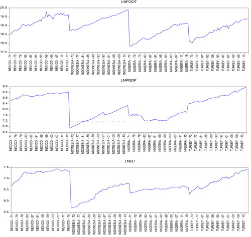
Figure 1 displays the graphical plots of the EF (LNFOOT), per capita real GDP (LNGDP), and energy usage (LNEC). It is seen that the data for all countries are in an upward trend in the given period.

Figure 1. The graphical plots of the natural logarithms of FOOT, PGDP, and EC.

Source: generated by the authors.

The logarithms of the variables to be analyzed can be expressed by panel regression as follows; (1) $$\text{ln}\hspace{0.17em}\mathit{foo}{t}_i{}_t={\beta }_0+{\beta }_1\hspace{0.17em}\text{ln}\hspace{0.17em}\mathit{pgd}{p}_{it}+{\beta }_2\hspace{0.17em}\text{ln}\hspace{0.17em}e{c}_{it}+{\epsilon }_{it}$$(1)

In the equation, i (i = 1, 2…N) represent the countries, t (t = 1.2…T) is the periods, and ε represent the disruptive term.

3.1. Panel vector auto regression

The panel vector autoregression (PVAR) approach has several practical benefits making it a better technique for analyzing macroeconomic fluctuations. First, the PVAR method is neutral to growth or development theories; it is based on the contemporaneous fluctuations of time series and not on a mathematical theorem of macroeconomics, which could be misrepresented if not acknowledged (Kireyev, 2000). Second, the current PVAR does not distinguish endogenous and exogenous variables; instead, all variables are considered endogenous. Every PVAR variable depends on all other variables, which indicate a real synchronism between the variables and their transaction. Then, PVAR offers a method for endogenous and exogenous shocks, which are certainly the most major sources of macroeconomic patterns for small open economies. Moreover, for consistent and efficient projections for both cases, PVAR is reasonably straightforward: A panel of countries or one country. Finally, PVAR has a precise, realistic estimate as a valuable tool for examining the joint impact of energy usage and real gross domestic product on the MINT countries' EF and providing strategic advice.

The linear equation of a P order, k-variable PVAR model shown in the panel-specific fixed effect format can be shown as follows; (2) $$y_i{}_t=y_{it-1}{A}_1+y_{it-2}{A}_2+\dots .+y_{it-p}{}_{+1}{A}_{p-1}+y_{it-p}{A}_p+x_{it}B+u_{it}+e_{it}$$(2) iϵ(1,2…N), tϵ(1,2…Ti). In the Equation, Yit shows the dependent variables vector (1xk), while Xit shows the external variables vector (1xk), and uit and eit represent 1xk dimensional effects and idiosyncratic vectors for error terms. The 1xk sized B and A1, A2…Ap-1, Ap vectors are estimated, as shown in the equation.

The structure of the variables in vector error correction models (VECM) is redesigned according to the PVAR equation (2)(2) $$y_i{}_t=y_{it-1}{A}_1+y_{it-2}{A}_2+\dots .+y_{it-p}{}_{+1}{A}_{p-1}+y_{it-p}{A}_p+x_{it}B+u_{it}+e_{it}$$(2) to construct the panel vector error correction model (PVECM); (3) $$\begin{array}{c}\Delta \hspace{0.17em}\text{ln}\hspace{0.17em}\mathit{foo}{t}_i{}_t=c_{1i}+\sum _{j=1}^q{\beta }_{11}{}_{ij}\Delta \hspace{0.17em}\text{ln}\hspace{0.17em}\mathit{foo}{t}_{it}{}_{-j}+\sum _{j=1}^q{\beta }_{12ij}\Delta \hspace{0.17em}\text{ln}\hspace{0.17em}\mathit{pgd}{p}_{it-j}+\sum _{j=1}^q{\beta }_{13ij}\Delta \hspace{0.17em}\text{ln}\hspace{0.17em}e{c}_{it-j}+{\beta }_{14i}{\epsilon }_i{}_{t-1}+u_{1it}\\ \Delta \hspace{0.17em}\text{ln}\hspace{0.17em}\mathit{pgd}{p}_i{}_t=c_{2i}+\sum _{j=1}^q{\beta }_{21ij}\Delta \hspace{0.17em}\text{ln}\hspace{0.17em}\mathit{foo}{t}_{it}{}_{-j}+\sum _{j=1}^q{\beta }_{22ij}\Delta \hspace{0.17em}\text{ln}\hspace{0.17em}\mathit{pgd}{p}_{it-j}+\sum _{j=1}^q{\beta }_{23ij}\Delta \hspace{0.17em}\text{ln}\hspace{0.17em}e{c}_{it-j}+{\beta }_{24i}{\epsilon }_i{}_{t-1}+u_{2it}\\ \Delta \hspace{0.17em}\text{ln}\hspace{0.17em}e{c}_i{}_t=c_{3i}+\sum _{j=1}^q{\beta }_{31ij}\Delta \hspace{0.17em}\text{ln}\hspace{0.17em}\mathit{foo}{t}_{it}{}_{-j}+\sum _{j=1}^q{\beta }_{32ij}\Delta \hspace{0.17em}\text{ln}\hspace{0.17em}\mathit{pgd}{p}_{it-j}+\sum _{j=1}^q{\beta }_{33ij}\Delta \hspace{0.17em}\text{ln}\hspace{0.17em}e{c}_{it-j}+{\beta }_{34i}{\epsilon }_i{}_{t-1}+u_{3it}\end{array}$$(3)

In which the first difference is Δ, q is the lag size, is error corrections, and u is the random error. The lag criteria are used to search for the optimum values for the lag. When each time series is I(1), and the variables are cointegrated, then a panel VECM may be utilized to measure causality, similar to what Engle and Granger (1987) follow. It is important to identify the cointegration between the variables. Since an error correction mechanism is ensured, shifts in the dependent variable form are a function of the level of relationship in the cointegration correlation and variations in other independent variables. The VECM is predicted using a seemengly unrelated regression (SUR) method that permits the residuals to have cross-sectional specific coefficients and cross-sectional relations.

3.2. Panel unit root test

Assessment of all stationarity data is required before progressing with the PVAR structure. There are two types of stationarity tests for the panel data: One accepts cross-sectional independence, and the other does not (Barbieri, 2006). The first type comprises Levin et al. (2002); Im et al. (2003); Maddala and Wu (1999); and Hadri (2000); panel stationarity tests, while the other includes Pesaran (2007); Bai and Ng (2004), Moon and Perron (2004), and Smith et al. (2004). However, first-type panel stationarity tests result in inaccurate and incorrect outcomes due to size distortions where substantial positive residual cross-section dependency levels occur and are not considered (Maddala & Wu, 1999). Thus, testing for the cross-sectional dependence in a panel study is vital to select the pertinent estimator.

In this study, Bai and Ng (2004) Panel Analysis of Nonstationarity in Idiosyncratic and Common Components (PANIC) and Pesaran's (2007) Cross-sectionally Augmented IPS (CIPS) tests will be used for cross-sectional dependency or second-generation unit root testing.

3.3. Panel cointegration tests

Panel cointegration tests are performed to assess whether the correlation between nonstationary variables represents a long-run relationship. The keen interest in and accessibility of panel data has diverted to a focus on the extension to panel data of various statistical tests. Current literature in a panel setting has focused on the assessment of cointegration. In this study, one of the following cointegration test types for panels will be estimated: Pedroni (1999, 2004), Kao (1999), a Fisher-type test using Johansen methodology (Maddala & Wu, 1999), Levin et al. (2002), Breitung (2000), Im et al. (2003), a Fisher-type test using ADF and PP tests Maddala and Wu (1999); Choi (2001); and Hadri (2000).

4. Empirical findings

4.1. Panel unit root

The panel stationarity tests are used to see if the data have the unit root. The outcomes of these tests are given in the first part of Table 2. Stationarity tests are examined for both the normal and the differentiated series in two different cases; series with a constant only and series with a constant and a trend together. Assuming stationarity, the null hypothesis is defined at the common and individual levels. For the LNEC series, in case only the constant exists, the unit root is rejected at a 5% level for the Im, Pesaran, and Shin W-sta test and a significance level of 1% for the other tests. However, the same tests predict that the series contains stationarity; therefore, the null hypothesis is accepted when the series contains the constant with the trend. So the series is not stationary. For the LNFOOT series, when only the constant exists, the series contains a unit root; however, when a trend and constant exist, the null hypothesis is rejected with at least a level of 5% in all tests except the Levin et al. (2002) t stationarity test. The LNPGDP series, on the other hand, accepts the null hypothesis when only the constant and the constant with the trend exist. In other words, the unit root exists both individually and in general terms. According to these results, it is understood that all series contain a unit root. In the second place, to see whether these series are integrated, it is necessary to look at the similarly differentiated states of these series.

Table 2. Cross-sectionally independent panel unit root tests.

	intercept			intercept and trend			intercept			intercept and trend			intercept			intercept and trend
Method	Statistic	Prob.**	Obs	Statistic	Prob.**	Obs	Statistic	Prob.**	Obs	Statistic	Prob.**	Obs	Statistic	Prob.**	Obs	Statistic	Prob.**	Obs
	Series: LNEC						Series: LNFOOT						Series: LNPGDP
Null: Unit root (assumes common unit root process)
Levin, Lin & Chu t*	−353.607	0.0002	180	−136.011	0.0869	179	−0.62878	0.2647	178	−0.64757	0.2586	179	−0.3360	0.3684	179	0.28470	0.6121	179
Breitung t-stat				1.61835	0.9472	175				−192.861	0.0269	175				−0.01134	0.4955	175
Null: Unit root (assumes individual unit root process)
Im, Pesaran and Shin W-stat	−202.906	0.0212	180	−106.740	0.1429	179	1.39686	0.9188	178	−184.368	0.0326	179	1.52955	0.9369	179	0.30268	0.6189	179
ADF - Fisher Chi-square	21.8751	0.0052	180	13.8395	0.0860	179	3.78592	0.8759	178	19.6041	0.0119	179	4.47523	0.8119	179	7.40504	0.4936	179
PP - Fisher Chi-square	21.0912	0.0069	180	11.7720	0.1617	180	3.45430	0.9027	180	22.7336	0.0037	180	4.23417	0.8354	180	6.88194	0.5494	180
	Series: D(LNEC)						Series: D(LNFOOT)						Series: D(LNPGDP)
Null: Unit root (assumes common unit root process)
Levin, Lin & Chu t*	−113.358	0.0000	176	−116.564	0.0000	176	−173.987	0.0000	176	−172.313	0.0000	176	−796.596	0.0000	175	−676.962	0.0000	170
Breitung t-stat				−801.502	0.0000	172				−794.248	0.0000	172				−762.102	0.0000	166
Null: Unit root (assumes individual unit root process)
Im, Pesaran and Shin W-stat	−984.940	0.0000	176	−971.237	0.0000	176	−168.221	0.0000	176	−168.888	0.0000	176	−772.780	0.0000	175	−672.162	0.0000	170
ADF - Fisher Chi-square	90.4635	0.0000	176	81.1068	0.0000	176	152.016	0.0000	176	183.477	0.0000	176	69.1085	0.0000	175	55.5408	0.0000	170
PP - Fisher Chi-square	90.9644	0.0000	176	82.6485	0.0000	176	145.015	0.0000	176	391.199	0.0000	176	78.9684	0.0000	176	65.8214	0.0000	176

Source: generated by the authors.

The second part of Table 2 shows the unit root tests in which the differences have been taken. The panel series's unit root test lags, whose differences are taken as Δ(x), are automatically selected on the SIC basis. The predictive results of each series that contain constant only and constant with trends together are included in the table. It is understood that the first order I(1) of the series is integrated for each estimation method for every differentiated series. The null hypothesis is rejected at 1% for all series. In other words, it is concluded that there is stationarity in the series that first-order difference has been taken. PVAR models analysis of the series whose first differences are stationary can be examined. If there is a long-term cointegration correlation in the series, it is essential to make a VECM estimate. Thus, the error correction equation showing long-term correlation can be obtained in the series.

The first generation unit root tests applied to the earlier panel data cannot fully identify the cross-sectional data affected by common factors. The second-generation panel unit root tests are used for cross-sectional dependence. This study utilizes EViews to investigate two crucial second-generation contributions: Bai and Ng (2004) PANIC and Pesaran's (2007) CIPS. In Table 3, cross-sectional dependency test results are reported according to Bai and Ng (2004). The deterministic terms included in the specification are listed as None, Constant, or Constant and trend. However, two of them are included here. In addition, automatic factor selection with MQC statistics which enables the Long-Run Variance Options, is preferred.

Table 3. Bai & Ng's panel unit root tests with cross-sectional dependence-PANIC.

Series: LNEC	Cross-sections: 4		Balanced observations: 45	Total observations: 180
Null hypothesis: Retain common factors
Common trends	Test statistic	p-value	Common trends	Test statistic	p-value
3	9.25761	0.99990	3	109.45342	0.99990
Idiosyncratic elements: Pooled test		Null hypothesis: No cointegration among all cross-sections
Lag selection: AIC with maxlag = 3, Test vari. MQC	Value	p-value		Value	p-value
Pooled statistic	4.0856	0.0004	Pooled statistic	2.9396	0.0032
Series: LNFOOT
Null hypothesis: Retain common factors
Common trends	Test statistic	p-value	Common trends	Test statistic	p-value
3	8.88938	0.99990	3	399.77742	0.99990
Idiosyncratic elements: Pooled test		Null hypothesis: No cointegration among all cross-sections
Lag selection: AIC with maxlag = 3	Value	p-value		Value	p-value
Pooled statistic	−1.97058	0.04877	Pooled statistic	2.62527	0.00866
Series: LNPGDP
Null hypothesis: Retain common factors
Common trends	Test statistic	p-value	Common trends	Test statistic	p-value
3	10.43055	0.99990	3	40.35603	0.99990
Idiosyncratic elements: Pooled test		Null hypothesis: No cointegration among all cross-sections
Lag selection: AIC with maxlag = 3	Value	p-value		Value	p-value
Pooled statistic	3.43620	0.00059	Pooled statistic	4.01561	0.00006

Source: generated by the authors.

Reports on LNEC, LNFOOT, and LNPGDP series are given in the table, respectively. At the top of the table, Bai and Ng (2004) PANIC deterministic test results for constant and constant with trend models of the LNEC series are given. The first line contains the individual results, and the second line provides the pooled test results. The null hypothesis, defined as “retain common factors” for the first test, is accepted with a very high score indicating permanent common factors in cross-section series. The same results were obtained for both constant and constant with trend models. For the pooled test presented in the second line, the null hypothesis, “no cointegration among all cross-sections,” is rejected again, indicating a cointegrated relationship among variables at the 1% significance level for both models. Similar results are found for the LNFOOT and the LNPGDP series; however, the pooled test result of the LNFOOT series indicates that the null hypothesis is rejected at the 5% significance level. According to these results, the existence of a cointegrated relationship between cross-section data is confirmed. Pesaran (2007) CIPS, one of the second-generation tests, is presented in Table 4.

Table 4. Pesaran's panel unit root tests with cross-sectional dependence-CIPS.

Deterministics: Constant					Deterministics: Constant and Trend
Series: LNEC
CIPS unit root test					CIPS unit root test
Null hypothesis: Unit root					Null hypothesis: Unit root
Statistic		t-stat	p-value		Statistic		t-stat	p-value
CIPS:		−232109	<0.10		CIPS:		−303235	<0.05
Truncated CIPS:		−232109	<0.10		Truncated CIPS:		−303235	<0.05
Critical values:					Critical values:
Level		CIPS	Trunc. CIPS		Level		CIPS	Trunc. CIPS
0,01		−2.56	−2.56		0,01		−3.07	−3.07
0,05		−2.33	−2.33		0,05		−2.85	−2.85
0,1		−2.21	−2.21		0,1		−2.73	−2.73
Cross-sectional ADF unit root test					Cross-sectional ADF unit root test
Null hypothesis: Unit root for specified cross-section					Null hypothesis: Unit root for specified cross-section
Lag selection: AIC with maxlag = 3					Lag selection: AIC with maxlag = 3
		CADF		Truncated CADF				CADF		Truncated CADF
Cross-section	ADF lags	t-stat	p-value	t-stat	p-value	Cross-section	ADF lags	t-stat	p-value	t-stat	p-value
MEXICO	1	−1.93.218	> =.10	−1.93.218	> =0.10	MEXICO	0	−3.56.994	<0.10	−3.56.994	<0.10
INDONESIA	0	−3.01.199	<0.10	−3.01.199	<0.10	INDONESIA	0	−2.61.288	> =.10	−2.61.288	> =0.10
NIGERIA	1	−2.25.779	> =.10	−2.25.779	> =0.10	NIGERIA	0	−2.11.486	> =.10	−2.11.486	> =0.10
TURKEY	1	−2.08.239	> =.10	−2.08.239	> =0.10	TURKEY	1	−3.83.174	<0.05	−3.83.174	<0.05
Critical values:						Critical values:
Level		CADF	Trunc. CADF			Level		CADF	Trunc. CADF
1%		−3.98	−3.98			1%		−4.54	−4.54
5%		−3.31	−3.31			5%		−3.80	−3.80
10%		−2.95	−2.95			10%		−3.45	−3.45
Series: LNFOOT
CIPS unit root test					CIPS unit root test
Null hypothesis: Unit root					Null hypothesis: Unit root
Statistic		t-stat	p-value		Statistic		t-stat	p-value
CIPS:		−227256	<0.10		CIPS:		−383782	<0.01
Truncated CIPS:		−227256	<0.10		Truncated CIPS:		−383782	<0.01
Critical values:					Critical values:
Level		CIPS	Trunc. CIPS		Level		CIPS	Trunc. CIPS
0,01		−2.56	−2.56		0,01		−3.07	−3.07
0,05		−2.33	−2.33		0,05		−2.85	−2.85
0,1		−2.21	−2.21		0,1		−2.73	−2.73
Cross-sectional ADF unit root test					Cross-sectional ADF unit root test
Null hypothesis: Unit root for specified cross-section					Null hypothesis: Unit root for specified cross-section
Lag selection: AIC with maxlag = 3					Lag selection: AIC with maxlag = 3
		CADF		Truncated CADF				CADF		Truncated CADF
Cross-section	ADF lags	t-stat	p-value	t-stat	p-value	Cross-section	ADF lags	t-stat	p-value	t-stat	p-value
MEXICO	1	−1.63.666	> =.10	−1.63.666	> =0.10	MEXICO	3	−4.64.498	<0.01	−4.64.498	<0.01
INDONESIA	0	−1.93.739	> =.10	−1.93.739	> =0.10	INDONESIA	0	−3.00.837	> =.10	−3.00.837	> =0.10
NIGERIA	0	−2.64.390	> =.10	−2.64.390	> =0.10	NIGERIA	0	−2.55.921	> =.10	−2.55.921	> =0.10
TURKEY	3	−2.87.229	> =.10	−2.87.229	> =0.10	TURKEY	3	−5.13.870	<0.01	−5.13.870	<0.01
Critical values:						Critical values:
Level		CADF	Trunc. CADF			Level		CADF	Trunc. CADF
1%		−3.98	−3.98			1%		−4.54	−4.54
5%		−3.31	−3.31			5%		−3.80	−3.80
10%		−2.95	−2.95			10%		−3.45	−3.45
Series: LNPGDP
CIPS unit root test					CIPS unit root test
Null hypothesis: Unit root					Null hypothesis: Unit root
Statistic		t-stat	p-value		Statistic		t-stat	p-value
CIPS:		−215643	> =0.10		CIPS:		−123503	> =0.10
Truncated CIPS:		−215643	> =0.10		Truncated CIPS:		−123503	> =0.10
Critical values:					Critical values:
Level		CIPS	Trunc. CIPS		Level		CIPS	Trunc. CIPS
0,01		−2.56	−2.56		0,01		−3.07	−3.07
0,05		−2.33	−2.33		0,05		−2.85	−2.85
0,1		−2.21	−2.21		0,1		−2.73	−2.73
Cross-sectional ADF unit root test					Cross-sectional ADF unit root test
Null hypothesis: Unit root for specified cross-section					Null hypothesis: Unit root for specified cross-section
Lag selection: AIC with maxlag = 3					Lag selection: AIC with maxlag = 3
		CADF		Truncated CADF				CADF		Truncated CADF
Cross-section	ADF lags	t-stat	p-value	t-stat	p-value	Cross-section	ADF lags	t-stat	p-value	t-stat	p-value
MEXICO	0	−2.53.358	> =.10	−2.53.358	> =0.10	MEXICO	0	−1.10.060	> =.10	−1.10.060	> =0.10
INDONESIA	0	−1.74.724	> =.10	−1.74.724	> =0.10	INDONESIA	0	−0.95123	> =.10	−0.95123	> =0.10
NIGERIA	0	−2.34.638	> =.10	−2.34.638	> =0.10	NIGERIA	0	0.58294	> =.10	0.58294	> =0.10
TURKEY	0	−1.99.852	> =.10	−1.99.852	> =0.10	TURKEY	1	−347.121	<0.10	−3.47.121	<0.10
Critical values:						Critical values:
Level		CADF	Trunc. CADF			Level		CADF	Trunc. CADF
1%		−3.98	−3.98			1%		−4.54	−4.54
5%		−3.31	−3.31			5%		−3.80	−3.80
10%		−2.95	−2.95			10%		−3.45	−3.45

Source: generated by the authors.

The first part of Table 4 lists the details of the CIPS test for the LNEC, LNFOOT, and LNLNPGDP variables. In particular, the first part of this table displays the critical values for the usual CIPS statistic and its truncated version. The second portion of this table summarizes the test results. Note that the t-statistic is displayed along with the associated p-values summarized categorically based on the critical values tabulated in Pesaran (2007). The suggestion for the null hypothesis indicating the existence of a unit root is the same for all three variables. The null hypothesis cannot be rejected below the 10% significance level. The first portion of the second part of the table summarizes the critical values associated with the CADF statistic and its truncated version. Finally, the second portion summarizes the test results for each of the cross-sections. In particular, these are t-statistics associated with the cross-sectionally augmented ADF regressions for each of the cross-sections. It is more convenient to evaluate it as a whole rather than specifying individual results for each country. The table summarizes the t-statistic and p-value category for each of the CADF and truncated CADF test statistics. In particular, here, the unit root null hypotheses cannot be rejected at significance levels less than 10% for any of the cross-sections.

4.2. Panel cointegration tests

In Table 5, the cointegration tests conducted to question the long-term correlation between the series are reported for two different situations. In the first part of the table showing the results without the trend, the null hypothesis is accepted, claiming no cointegration correlation between the series according to the panel v and panel ADF statistics. According to the other two test results, the null hypothesis of the series is rejected at a 5% level; there is a cointegration correlation. According to the group ADF-Statistic test result in the group cointegration, the null hypothesis that predicts no cointegrated correlation between the series is accepted. In contrast, the other two tests are rejected at a 1% significance level. As a result, in four of the seven tests, a cointegrated correlation between these series exists.

Table 5. Pedroni residual cointegration test.

Series: LNFOOT, LNPGDP, LNEC
Null Hypothesis: No cointegration
Trend assumption: No deterministic trend
Alternative hypothesis: common AR coefs. (within-dimension)
	Statistic		Prob.	Weighted Statist.		Prob.
Panel v-Statistic	0.815923		0.2073	0.723673		0.2346
Panel rho-Statistic	−2.086909		0.0184	−1.787337		0.0369
Panel PP-Statistic	−2.188876		0.0143	−2.097189		0.0180
Panel ADF-Statistic	0.162070		0.5644	−0.434520		0.3320
Alternative hypothesis: individual AR coefs. (between-dimension)
Group rho-Statistic	Statistic		Prob.
Group PP-Statistic	−2.511430		0.0060
Group ADF-Statistic	−3.004358		0.0013
	−0.497835		0.3093
Null Hypothesis: No cointegration
Trend assumption: Deterministic and constant exist
Alternative hypothesis: common AR coefs. (within-dimension)
Panel v-Statistic	Statistic	Prob.		Weighted Stat.	Prob.
Panel rho-Statistic	1.256255	0.1045		1.339767	0.0902
Panel PP-Statistic	−3.096976	0.0010		−2.962420	0.0015
Panel ADF-Statistic	−3.421997	0.0003		−3.629691	0.0001
	0.584522	0.7206		−0.717643	0.2365
Alternative hypothesis: individual AR coefs. (between-dimension)
Group rho-Statistic	Statistic	Prob.
Group PP-Statistic	−2.125741	0.0168
Group ADF-Statistic	−3.140628	0.0008
	−0.396845	0.3457

Source: generated by the authors.

The cointegration test results performed in a deterministic trend are given in the second part of Table 5. The results for the trend and constant are similar to the results in previous ones; the null hypothesis is accepted, implying that there is no cointegrated correlation between the series according to the panel v and panel ADF test statistic. According to the other two test results, the null hypothesis is rejected at a 1% level, implying a cointegrated correlation. In the case of a deterministic trend, the same conclusions are reached. According to the group ADF-statistic test result, the null is accepted at a 1% level in group cointegration. In comparison, the null is rejected at a 5% level for the group rho-statistic and group pp-statistic tests. As a result, four out of seven tests indicate a cointegrated correlation between these series.

The panel cointegration test results of Johansen Fisher are given in Table 6. The null hypothesis is defined as no cointegration correlation. According to the result of the tests, there is at least one cointegrate vector at a 1% significance level according to the trace test and at least a 5% significance level according to the max-eigen test results.

Table 6. Johansen Fisher panel cointegration test.

Series: LNFOOT LNPGDP LNEC
Trend assumption: No deterministic trend
Hypothesized	Fisher Stat.*		Fisher Stat.*
No. of CE(s)	(from trace test)	Prob.	(from max-eigen test)	Prob.
None	21.50	0.0059	19.33	0.0132
At most 1	10.92	0.2060	8.390	0.3963
At most 2	11.78	0.1614	11.78	0.1614

* Probabilities are computed using asymptotic Chi-square distribution.

Source: generated by the authors.

4.3. Vector error correction model

From the unit root and cointegration tests performed up to this point, it is understood that the series contains stationarity, and there is a long-term correlation between the series. In such a case, the cointegrated vector can be obtained by estimating VECM as formulated earlier in (3). However, when predicting PVAR estimation, the most suitable lag size can be determined in advance. Table 7 shows the analysis for lag size. The length of the lag, which indicates that the model estimate is the most suitable, is evaluated for five different criteria. The most suitable lag size for PVAR analysis in five criteria is listed in the table as two, and therefore, the lag size of the model in this work should be determined to be two as suggested.

Table 7. VAR lag size criteria.

Endogenous variables: LNFOOT LNPGDP LNEC
Lag	LogL	LR	FPE	AIC	SC	HQ
0	−200.4504	NA	0.002919	2.676979	2.736661	2.701224
1	799.9768	1948.200	6.31e-09	−10.36812	−10.12939	−10.27114
2	825.3007	48.31539*	5.09e-09*	−10.58290*	−10.16513*	−10.41319*
3	830.7196	10.12485	5.34e-09	−10.53578	−9.938966	−10.29334
4	835.6897	9.090026	5.63e-09	−10.48276	−9.706895	−10.16758
5	842.2310	11.70549	5.82e-09	−10.45041	−9.495499	−10.06249
6	844.6132	4.168823	6.36e-09	−10.36333	−9.229376	−9.902680
7	851.3131	11.46032	6.57e-09	−10.33307	−9.020066	−9.799680
8	859.0595	12.94474	6.70e-09	−10.31657	−8.824527	−9.710452

* indicates lag order selected by the criterion.

LR: sequential modified LR test statistic (each test at 5% level).

FPE: Final prediction error.

AIC: Akaike information criterion.

SC: Schwarz information criterion.

HQ: Hannan-Quinn information criterion.

Source: generated by the authors.

The results of VECM estimates for two lags are shown in Table 8. It can be seen from the coefficient estimates of the cointegrating vector that there is at least one cointegrate vector between the series. In the test for restrictions on Engle and Granger (1987) cointegrated vectors, the “nxk” dimensional αβ-matrix is defined by Johansen (1988). It is expressed in the form of π = αβ' matrix where β represents the cointegration parameter matrix, and α matrix represents the weights of cointegrate vectors included in the n-equation VAR model. In other words, α constitutes the matrix of velocity adjustment parameters. If the elements of the π matrix, long-term variables, are equal to zero, equation (2)(2) $$y_i{}_t=y_{it-1}{A}_1+y_{it-2}{A}_2+\dots .+y_{it-p}{}_{+1}{A}_{p-1}+y_{it-p}{A}_p+x_{it}B+u_{it}+e_{it}$$(2) is a first-order VAR equation. In this case, there is no error correction representation.

Table 8. Vector error correction model estimates (α and β vectors).

Sample (adjusted): 1974 2016; Standard errors in ( ) & t-statistics in [ ]
$\pi =\alpha {\beta }^{\prime }$
Error Correction:
$\alpha$	−0.023939	0.014827	0.011737
	(0.01005)	(0.00703)	(0.00588)
	[-2.38174]	[ 2.10850]	[ 1.99609]
$\beta$
LNFOOT(-1)	LNPGDP(-1)	LNEC(-1)	C
1.000000	0.914821	−2.223.179	−1.146.941
	(0.27762)	(0.51187)
	[ 3.29524]	[-4.34329]

Source: generated by the authors.

As can be seen from the table, t statistical values are at least equal to two, which means that these coefficients are significant at least a 5% significance level and confirm the cointegrated vector's existence. Similarly, the fact that these coefficients are different from zero indicates that the long-term Granger causality test predicts a causal correlation between the series.

An essential part of short-term coefficients in VECM analysis does not seem statistically significant. Only the t statistical value of the short-term coefficient is higher than two. The dependent variable of D(LNFOOT(-1)) is significant at the 1% level in the equation. The dependent variable of D(LNPGDP(-1)) is significant at less than 5% in the equation. According to Akaike AIC and Schwarz SC criteria, it has been determined that the predicted model is the most suitable compared to the trend-containing prediction model with the same lag size (Table 9).

Table 9. Short term estimates (t-statistics in [ ]).

	D(LNFOOT)	D(LNPGDP)	D(LNEC)
D(LNFOOT(-1))	−0.498888**	−0.085540	−0.041276
	[-5.79435]	[-1.42007]	[-0.81950]
D(LNFOOT(-2))	−0.144671	−0.080382	0.004661
	[-1.71958]	[-1.36565]	[ 0.09470]
D(LNPGDP(-1))	0.194263	0.183964	0.071632
	[ 1.51465]	[ 2.05019]*	[ 0.95472]
D(LNPGDP(-2))	0.213153	0.111627	−0.061814
	[ 1.66855]	[ 1.24898]	[-0.82714]
D(LNEC(-1))	0.107052	0.125002	0.102796
	[ 0.70342]	[ 1.17402]	[ 1.15463]
D(LNEC(-2))	0.039809	−0.044169	0.012619
	[ 0.26759]	[-0.42437]	[ 0.14500]
C	0.034319	0.016764	0.014728
	[ 5.68887]**	[ 3.97211]*	[ 4.17351]**
R-squared	0.203036	0.136222	0.057029
Log-likelihood	245.5479	306.9899	337.7657
Akaike AIC	-2.762.185	-3.476.626	-3.834.485

(**) %1, (*) meaningful at the level of %5 significance.

Source: generated by the authors.

4.4. Impulse-response functions

The outcomes of the analysis by the impulse-response functions (IRFs) of EC, PGDP, and FOOT are presented and discussed here. As discussed earlier, choosing the correct order of variables is a crucial step when studying the IRFs. The IRFs in the PVAR model, developed by Love and Zicchino (2006), are focused on the Cholesky decomposition of the variance-covariance residue matrix proposed by Sims (1980) to ensure orthogonalization of shocks.

Impulse-response functions of LNFOOT, LNPGDP, and LNEC are given in Figure 2. The response function of each variable against one standard deviation shock in each variable is given for ten lags with a 5% interval band. The reactions of LNFOOT to shocks in itself, LNPGDP, and LNEC series are illustrated at the top of the figure. As seen in the first graph in the figure, LNFOOT's response to its own change is positive and downward. However, it continues to decrease slightly over time.

Figure 2. Impulse response functions.

Source: generated by the authors.

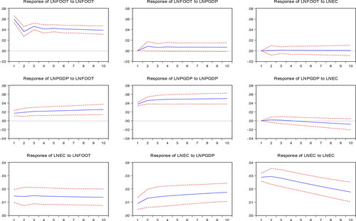
Similarly, LNFOOT responses to a shock in the LNPGDP and LNEC series in the first two periods are also positive. However, the reaction to LNPGDP then continues without increasing. LNFOOT's response to the change in the LNEC continues close to zero throughout the period.

The second row of graphs shows the LNPGDP series's response to a shock in LNFOOT, itself, and LNEC series. The reaction of the LNPGDP series to LNFOOT and to itself remains on a positive scale of a specific size starting from the first period. There is no significant increase. While the response of LNPGDP to the change in the LNEC series is quite low at first, it reacts negatively after the sixth lag. It should be noted that this is considered as a cost element and that per capita income responds negatively.

The graphs in the last line show the response of the LNEC series to itself and the other two series for ten lags. It can be said that the response of LNEC's to the shocks in the LNFOOT variable during the entire period is on the positive plane and rarely changed. The reaction of LNEC to shock change in LNPGDP is in a positive plane and tends to increase slightly throughout the period. Its reaction to a shock in itself, on the other hand, tends to decrease only in a positive plane.

4.5. Short-run and log-run dynamics: granger causality

Two features are expected in the adjustment coefficients (α) for a long-run causal relationship. These coefficients must be statistically different from zero and have a negative sign. The Wald test results presented in Table 10 show that the initial adjustment coefficient is statistically significant with a negative sign and a 5% significance level. As given in the table below, the null hypothesis is rejected at a 1% significance level. It is understood that there is a long-term causal relationship between the variables.

Table 10. The Wald test results for long-term relationship among variables.

Test Statistic	Value	df	Probability
Chi-squire	12.22970	3	0.0066
Null Hypothesis: C(1)=C(9)=C(14)=0
Null Hypothesis Summary:
Normalized Restrictions (=0)		Value	Std. Err.
C(1)		−0.023939	0.010051
C(9)		0.011737	0.005880
C(14)		0.071632	0.075029
Restrictions are linear in coefficients.

Source: generated by the authors.

In the estimated VAR equation (2)(2) $$y_i{}_t=y_{it-1}{A}_1+y_{it-2}{A}_2+\dots .+y_{it-p}{}_{+1}{A}_{p-1}+y_{it-p}{A}_p+x_{it}B+u_{it}+e_{it}$$(2) , Engle and Granger (1987) is referred to the VAR Granger Causality/Block Exogeneity Wald test to determine the presence of a short-run causality correlation. Table 11 presents the estimations of the causality correlation of each variable whose differences are taken as the dependent variable. The vector autoregression lag size q is set at two and is determined using the Schwarz information criteria in all cases. In the short run, D(LNFOOT) is the Granger cause of D(LNPGDP) at only a 10% significance level. The coexistence of D(LNEC) and D(LNPGDP) is also seen as the Granger cause at the 10% significance level.

Table 11. VEC granger causality/block exogeneity Wald tests.

Excluded	Chi-sq	df	Prob.
Dependent variable: D(LNFOOT)
D(LNPGDP)	5.632514	2	0.0598
D(LNEC)	0.608328	2	0.7377
All	8.796465	4	0.0664
Dependent variable: D(LNPGDP)
D(LNFOOT)	2.778879	2	0.2492
D(LNEC)	1.476092	2	0.4780
All	3.813193	4	0.4319
Dependent variable: D(LNEC)
D(LNFOOT)	0.881559	2	0.6435
D(LNPGDP)	1.453817	2	0.4834
All	1.935382	4	0.7476

Source: generated by the authors.

4.6. Long-run dynamics: fully modified and dynamic OLS

Based on equation (2)(2) $$y_i{}_t=y_{it-1}{A}_1+y_{it-2}{A}_2+\dots .+y_{it-p}{}_{+1}{A}_{p-1}+y_{it-p}{A}_p+x_{it}B+u_{it}+e_{it}$$(2) , the output elasticities in the long-run are estimated using panel FMOLS and DOLS estimators (Kao & Chiang, 2000; Pedroni, 1999, 2004; Phillips & Moon, 1999; Saikkonen (1992) and Stock and Watson (1993)). FMOLS, canonical cointegrating regression, and DOLS estimators are asymptotic and have a normal distribution. Static OLS is a particular case of DOLS. The maximum likelihood approach of Johansen (1991, 1995) is stressed again.

Table 12 shows the long-run elasticities between variables. For both FMOLS and DOLS models, the estimated coefficient of LNPGDP appears to be statistically insignificant. However, that of LNEC is statistically significant at 1% for both models. The elasticity value of LNEC compared to LNFOOT appears to be 1.141. In other words, a 1 percent increase in LNEC increases the elasticity of LNFOOT by 1.141%. Considering the long term, the rise in energy usage increases the elasticity of the EF. Similar conclusions can be drawn from the FMOLS estimate. A 1% increase in the LNEC, the only variable with a statistically significant coefficient, increases the elasticity of LNFOOT by 1.197%.

Table 12. DOLS and FMOLS estimators.

Variable	Coefficient	Std. Error	t-Statistic	Prob.
Dependent Variable: LNFOOT
Method: Panel Dynamic Least Squares (DOLS)
LNPGDP	0.019335	0.208905	0.092553	0.9264
LNEC	1.141.962	0.247529	4.613.444	0.0000
R-squared	0.887630
Adjusted R-squared	0.864681
S.E. of regression	0.174224
Long-run variance	0.075537
Dependent Variable: LNFOOT
Method: Panel Fully Modified Least Squares (FMOLS)
LNPGDP	−0.036797	0.196600	−0.187169	0.8517
LNEC	1.197.881	0.235065	5.095.965	0.0000
R-squared	0.823285
Adjusted R-squared	0.818207
S.E. of regression	0.206911
Long-run variance	0.107241

Source: generated by the authors.

5. Results

This study investigates the correlation between energy usage, per capita GDP, and EF as an assessment for ecological deterioration for the MINT countries between 1976 and 2016. Second-generation unit root tests were applied to determine whether there is a cross-section dependency relationship within the series. Since the series becomes stationary, PVAR analysis with VECM investigates a possible long-term cointegration correlation. An essential part of short-term coefficients in VECM analysis does not seem statistically significant. The error correction equation determines that the variables are significant, and there is a positive and long-term correlation between energy usage and EF.

The impulse response processes of variables at certain lags are evaluated with the impulse response functions. EF's response to its shocks is positive and downward but decreases slightly over time. Similarly, EF's positive response to a standard deviation shock in the per capita real GDP and energy usage in the first two periods. However, the reaction to per capita real income then continues without increasing positively, and the reaction to the change in energy usage remains close to zero throughout the period. The Wald test detected the existence of a long-term causal relationship between the variables. The EF is the Granger cause of the per capita real income at only a 10% significance level. Also, real income is the Granger cause of energy usage in the short term. Furthermore, the coexistence of energy usage and income is also seen as the Granger cause at the 10% significance level.

Finally, the cointegration equation, which shows the long-term correlation between variables, is estimated using DOLS and FMOLS analysis. Similar results are obtained from the FMOLS and DOLS estimation; the estimated per capita real GDP coefficient seems insignificant. However, the estimated coefficient of energy usage is significant at 1% for both models. Considering the long term, a 1% increase in energy usage increases the elasticity of the EF, according to DOLS and FMOLS analysis. Only the increase in energy usage, whose coefficient is significant, increases the elasticity of the EF.

Contrary to existing studies (Bagliani et al., 2008; Caviglia-Harris et al., 2009; Hervieux & Darné, 2015; Wang et al., 2013), no significant relationship was found between economic growth and environmental degradation in the study. Though the existence of a one-sided and significant relationship from energy consumption to environmental degradation is supported by Ang (2007), Begum et al. (2015), Riti et al. (2017), and Le and Quah (2018). However, while the CO2 variable was used as an indicator of environmental degradation in these studies, the ecological footprint was used as a better indicator of environmental degradation in our study.

In this study, the relationship between growth, energy, and environment in the MINT country group was examined for the period 1976–2016. The relationship between these variables changed after 2016, especially during the covid 19 pandemic process, may be the subject of new studies. Besides, the effects of increases in ecological footprint on the formation of pandemics similar to the covid 19 pandemics can be considered a separate study.

According to DOLS results, when energy use increased by 1%, ecological footprint increased by 1.41%; According to FMOLS results, when energy use increases by 1%, it is seen that the ecological footprint increases by 1.197%. This cointegration relationship gives important clues for MINT countries. It is recommended that MINT countries implement policies that reduce fossil fuel resources and increase renewable energy resources in energy consumption.

Disclosure statement

No potential conflict of interest was reported by the authors.

References

- Abid, M. (2015). The close relationship between informal economic growth and carbon emissions in Tunisia since 1980: The (ir)relevance of structural breaks. Sustainable Cities and Society, 15, 11–21. https://doi.org/10.1016/j.scs.2014.11.001
- Ahmad, A., Zhao, Y., Shahbaz, M., Bano, S., Zhang, Z., Wang, S., & Liu, Y. (2016). Carbon emissions, energy consumption, and economic growth: An aggregate and disaggregate analysis of the Indian economy. Energy Policy, 96, 131–143. https://doi.org/10.1016/j.enpol.2016.05.032
- Ahmed, R. R., & Streimikiene, D. (2021). Environmental issues and strategic corporate social responsibility for organizational competitiveness. Journal of Competitiveness, 13(2), 5–22. https://doi.org/10.7441/joc.2021.02.01
- Ahmed, Z., Wang, Z., Mahmood, F., Hafeez, M., & Ali, N. (2019). Does globalization increase the ecological footprint? Empirical evidence from Malaysia. Environmental Science and Pollution Research International, 26(18), 18565–18582. https://doi.org/10.1007/s11356-019-05224-9
- Akpan, G. F., & Akpan, U. F. (2012). Electricity consumption, carbon emissions, and economic growth in Nigeria. International Journal of Energy Economics and Policy, 2 (4), 292–306.
- Al-Mulali, U., Weng-Wai, C., Sheau-Ting, L., & Mohammed, A. H. (2015). Investigating the environmental Kuznets curve (EKC) hypothesis by utilizing the ecological footprint as an indicator of environmental degradation. Ecological Indicators, 48, 315–323. https://doi.org/10.1016/j.ecolind.2014.08.029
- Alola, A. A., Bekun, F. V., & Sarkodie, S. A. (2019). Dynamic impact of trade policy, economic growth, fertility rate, renewable and non-renewable energy consumption on ecological footprint in Europe. The Science of the Total Environment, 685, 702–709. https://doi.org/10.1016/j.scitotenv.2019.05.139
- Alvarado, R., Ortiz, C., Jiménez, N., Ochoa-Jiménez, D., & Tillaguango, B. (2021). Ecological footprint, air quality and research and development: The role of agriculture and international trade. Journal of Cleaner Production, 288, 125589. https://doi.org/10.1016/j.jclepro.2020.125589
- Ang, J. B. (2007). CO2 emissions, energy consumption, and output in France. Energy Policy, 35(10), 4772–4778. https://doi.org/10.1016/j.enpol.2007.03.032
- Arouri, M. E. H., Ben Youssef, A., M'henni, H., & Rault, C. (2012). Energy consumption, economic growth and CO2 emissions in Middle East and North African countries. Energy Policy, 45, 342–349. https://doi.org/10.1016/j.enpol.2012.02.042
- Aşıcı, A. A., & Acar, S. (2016). Does income growth relocate ecological footprint? Ecological Indicators, 61(2), 707–714. https://doi.org/10.1016/j.ecolind.2015.10.022
- Asongu, S., Akpan, U. S., & Isihak, S. R. (2018). Determinants of foreign direct investment in fast-growing economies: Evidence from the BRICS and MINT countries. Financial Innovation, 4(1), 26. https://doi.org/10.1186/s40854-018-0114-0
- Bagliani, M., Bravo, G., & Dalmazzone, S. (2008). A consumption-based approach to environmental Kuznets curves using the ecological footprint indicator. Ecological Economics, 65(3), 650–661. https://doi.org/10.1016/j.ecolecon.2008.01.010
- Bai, J., & Ng, S. (2004). A panic attack on unit roots and cointegration. Econometrica, 72(4), 1127–1177. https://doi.org/10.1111/j.1468-0262.2004.00528.x
- Baloch, M. A., Zhang, J., Iqbal, K., & Iqbal, Z. (2019). The effect of financial development on ecological footprint in BRI countries: Evidence from panel data estimation. Environmental Science and Pollution Research International, 26(6), 6199–6208. https://doi.org/10.1007/s11356-018-3992-9
- Barbieri, L. (2006). Panel unit root tests: A review. Serie Rossa: Economia – Quaderno N. 43. Università Cattolica del Sacro Cuore.
- Begum, R. A., Sohag, K., Abdullah, S. M. S., & Jaafar, M. (2015). CO2 emissions, energy consumption, economic and population growth in Malaysia. Renewable and Sustainable Energy Reviews, 41, 594–601. https://doi.org/10.1016/j.rser.2014.07.205
- Bekun, F. V., Emir, F., & Sarkodie, S. A. (2019). Another look at the relationship between energy consumption, carbon dioxide emissions, and economic growth in South Africa. The Science of the Total Environment, 655, 759–765. https://doi.org/10.1016/j.scitotenv.2018.11.271
- Breitung, J. (2000). The local power of some unit root tests for panel data. In B. Baltagi (Ed.), Nonstationary panels, panel cointegration, and dynamic panels, advances in econometrics (Vol. 15, pp. 161–178). Emerald Group Publishing Limited.
- Caviglia-Harris, J. L., Chambers, D., & Kahn, J. R. (2009). Taking the ‘U' out of Kuznets. A comprehensive analysis of the EKC and environmental degradation. Ecological Economics, 68(4), 1149–1159. https://doi.org/10.1016/j.ecolecon.2008.08.006
- Charfeddine, L., & Mrabet, Z. (2017). The impact of economic development and social-political factors on ecological footprint: A panel data analysis for 15 MENA countries. Renewable and Sustainable Energy Reviews, 76, 138–154. https://doi.org/10.1016/j.rser.2017.03.031
- Chen, P. Y., Chen, S. T., Hsu, C. S., & Chen, C. C. (2016). Modeling the global relationships among economic growth, energy consumption, and CO2 emissions. Renewable and Sustainable Energy Reviews, 65, 420–431. https://doi.org/10.1016/j.rser.2016.06.074
- Choi, I. (2001). Unit root tests for panel data. Journal of International Money and Finance, 20(2), 249–272. https://doi.org/10.1016/S0261-5606(00)00048-6
- Destek, M. A., & Sarkodie, S. A. (2019). Investigation of environmental Kuznets curve for ecological footprint: The role of energy and financial development. The Science of the Total Environment, 650(Pt 2), 2483–2489. https://doi.org/10.1016/j.scitotenv.2018.10.017
- Destek, M. A., Ulucak, R., & Dogan, E. (2018). Analyzing the environmental Kuznets curve for the EU countries: The role of ecological footprint. Environmental Science and Pollution Research International, 25(29), 29387–29396. https://doi.org/10.1007/s11356-018-2911-4
- Engle, R., & Granger, C. (1987). Co-integration and error correction: Representation, estimation, and testing. Econometrica, 55(2), 251–276. https://doi.org/10.2307/1913236
- Fujii, H., & Managi, S. (2013). Which industry is greener? An empirical study of nine industries in OECD countries. Energy Policy, 57, 381–388. https://doi.org/10.1016/j.enpol.2013.02.011
- Galeotti, M., Manera, M., & Lanza, A. (2009). On the robustness of robustness checks of the environmental Kuznets curve hypothesis. Environmental and Resource Economics, 42 (4), 551–574. https://doi.org/10.1007/s10640-008-9224-x
- Gao, C., Zhu, S., An, N., Na, H., You, H., & Gao, C. (2021). Comprehensive comparison of multiple renewable power generation methods: A combination analysis of life cycle assessment and ecological footprint. Renewable and Sustainable Energy Reviews, 147, 111255. https://doi.org/10.1016/j.rser.2021.111255
- Global Footprint Network. (2020, January 6). Ecological Footprint (gha). http://data.footprintnetwork.org/
- Grossman, G. M., & Krueger, A. B. (1995). Economic growth and the environment. The Quarterly Journal of Economics, 110(2), 353–377. https://doi.org/10.2307/2118443
- Grossman, G. M., & Krueger, A. B. (1991). Environmental impacts of a North American free trade agreement. NBER Working Paper No. w3914, pp. 1–57.
- Hadri, K. (2000). Testing for stationarity in heterogeneous panel data. The Econometrics Journal, 3(2), 148–161. https://doi.org/10.1111/1368-423X.00043
- Halicioglu, F. (2009). An econometric study of CO 2 emissions, energy consumption, income, and foreign trade in Turkey. Energy Policy, 37(3), 1156–1164. https://doi.org/10.1016/j.enpol.2008.11.012
- Hervieux, M. S., & Darné, O. (2015). Environmental Kuznets curve and ecological footprint: A time series analysis. Economics Bulletin, 35(1), 814–826.
- Hwang, J. H., & Yoo, S. H. (2014). Energy consumption, CO2 emissions, and economic growth: Evidence from Indonesia. Quality & Quantity, 48 (1), 63–73. https://doi.org/10.1007/s11135-012-9749-5
- Im, K. S., Pesaran, M. H., & Shin, Y. (2003). Testing for unit roots in heterogeneous panels. Journal of Econometrics, 115(1), 53–74. https://doi.org/10.1016/S0304-4076(03)00092-7
- Jardón, A., Kuik, O., & Tol, R. S. J. (2017). Economic growth and carbon dioxide emissions: An analysis of Latin America and the Caribbean. Atmósfera, 30(2), 87–100. https://doi.org/10.20937/ATM.2017.30.02.02
- Johansen, S. (1988). Statistical analysis of cointegrating vectors. Journal of Economic Dynamics and Control, 12(2-3), 231–254. https://doi.org/10.1016/0165-1889(88)90041-3
- Johansen, S. (1991). Estimation and hypothesis testing of cointegration vectors in gaussian vector autoregressive models. Econometrica, 59(6), 1551–1580. https://doi.org/10.2307/2938278
- Johansen, S. (1995). Likelihood-based inference in cointegrated vector autoregressive models. Oxford University Press.
- Kao, C. (1999). Spurious regression and residual-based tests for cointegration in panel data. Journal of Econometrics, 90(1), 1–44. https://doi.org/10.1016/S0304-4076(98)00023-2
- Kao, C., & Chiang, M. H. (2000). On the estimation and inference of a cointegrated regression in panel data. In B. H. Baltagi (Eds.), Nonstationary panels, panel cointegration and dynamic panels (Vol. 15, pp. 179–222).Elsevier.
- Kasman, A., & Duman, Y. S. (2015). CO2 emissions, economic growth, energy consumption, trade and urbanization in new EU member and candidate countries: A panel data analysis. Economic Modelling, 44, 97–103. https://doi.org/10.1016/j.econmod.2014.10.022
- Ke, H., Dai, S., & Yu, H. (2021). Spatial effect of innovation efficiency on ecological footprint: City-level empirical evidence from China. Environmental Technology & Innovation, 22, 101536. https://doi.org/10.1016/j.eti.2021.101536
- Kireyev, A. P. (2000). Comparative macroeconomic dynamics in the Arab world: A panel VAR approach. IMF Working Papers WP/00/54. https://doi.org/10.5089/9781451847505.001
- Kraft, J., & Kraft, A. (1978). Relationship between Energy and GNP. The Journal of Energy and Development, 3(2), 401–403.
- Krkošková, R. (2021). Causality between energy consumption and economic growth in the V4 countries. Technological and Economic Development of Economy, 27(4), 900–920. https://doi.org/10.3846/tede.2021.14863
- Le, T. H., & Quah, E. (2018). Income level and the emissions, energy, and growth nexus: Evidence from Asia and the Pacific. International Economics, 156, 193–205. https://doi.org/10.1016/j.inteco.2018.03.002
- Levin, A., Lin, C. F., & Chu, C. (2002). Unit root tests in panel data: Asymptotic and finite-sample properties. Journal of Econometrics, 108(1), 1–24. https://doi.org/10.1016/S0304-4076(01)00098-7
- Love, I., & Zicchino, L. (2006). Financial development and dynamic investment behavior: Evidence from panel VAR. The Quarterly Review of Economics and Finance, 46(2), 190– 210. https://doi.org/10.1016/j.qref.2005.11.007
- Maddala, G. S., & Wu, S. (1999). A comparative study of unit root tests with panel data and a new simple test. Oxford Bulletin of Economics and Statistics, 61(S1), 631–652. https://doi.org/10.1111/1468-0084.0610s1631
- Moon, H. R., & Perron, B. (2004). Testing for a unit root in panel with dynamic factors. Journal of Econometrics, 122(1), 81–126. https://doi.org/10.1016/j.jeconom.2003.10.020
- Narayan, P. K., & Narayan, S. (2010). Carbon dioxide emissions and economic growth: Panel data evidence from developing countries. Energy Policy, 38(1), 661–666. https://doi.org/10.1016/j.enpol.2009.09.005
- Obradović, S., & Lojanica, N. (2017). Energy use, CO2 emissions, and economic growth-causality on a sample of SEE countries. Economic Research-Ekonomska Istraživanja, 30(1), 511–526. https://doi.org/10.1080/1331677X.2017.1305785
- Ozturk, I., & Acaravci, A. (2010). CO2 emissions, energy consumption, and economic growth in Turkey. Renewable and Sustainable Energy Reviews, 14(9), 3220–3225. https://doi.org/10.1016/j.rser.2010.07.005
- Ozturk, I., Al-Mulali, U., & Saboori, B. (2016). Investigating the environmental Kuznets curve hypothesis: The role of tourism and ecological footprint. Environmental Science and Pollution Research International, 23(2), 1916–1928. https://doi.org/10.1007/s11356-015-5447-x
- Pao, H. T., & Chen, C. C. (2019). Decoupling strategies: CO2 emissions, energy resources, and economic growth in the group of twenty. Journal of Cleaner Production, 206, 907–919. https://doi.org/10.1016/j.jclepro.2018.09.190
- Pao, H. T., & Tsai, C. M. (2011). Multivariate granger causality between CO2 emissions, energy consumption, FDI (foreign direct investment), and GDP (gross domestic product): Evidence from a Panel of BRIC (Brazil, Russian Federation, India, and China). Energy, 36(1), 685–693. https://doi.org/10.1016/j.energy.2010.09.041
- Pedroni, P. (1999). Critical values for cointegration tests in heterogeneous panels with multiple regressors. Oxford Bulletin of Economics and Statistics, 61(s1), 653–670. https://doi.org/10.1111/1468-0084.0610s1653
- Pedroni, P. (2004). Panel cointegration: Asymptotic and finite sample properties of pooled time series tests with an application to the PPP hypothesis: New results. Econometric Theory, 20(03), 597–625. https://doi.org/10.1017/S0266466604203073
- Pesaran, M. H. (2007). A simple panel unit root test in the presence of cross section dependence. Journal of Applied Econometrics, 22(2), 265–312. https://doi.org/10.1002/jae.951
- Phillips, P. C. B., & Moon, H. R. (1999). Linear regression limit theory for nonstationary panel data. Econometrica, 67(5), 1057–1111. https://doi.org/10.1111/1468-0262.00070
- Riti, J. S., Song, D., Shu, Y., & Kamah, M. (2017). Decoupling CO2 emission and economic growth in China: Is there consistency in estimation results in analyzing environmental Kuznets curve? Journal of Cleaner Production, 166, 1448–1461. https://doi.org/10.1016/j.jclepro.2017.08.117
- Rus, A. V., Rovinaru, M. D., Pirvu, M., Bako, E. D., & Rovinaru, F. I. (2020). Renewable energy generation and consumption across 2030-analysis and forecast of required growth in generation capacity. Transformations in Business & Economics, 19(2B), 746–766.
- Saikkonen, P. (1992). Estimation and testing of cointegrated systems by an autoregressive approximation. Econometric Theory, 8(01), 1–27. https://doi.org/10.1017/S0266466600010720
- Shahbaz, M., Hye, G. M. A., Tiwari, A. K., & Leitão, N. C. (2013). Economic growth, energy consumption, financial development, international trade and CO2 emissions in Indonesia. Renewable and Sustainable Energy Reviews, 25, 109–121. https://doi.org/10.1016/j.rser.2013.04.009
- Shao, J., Tillaguango, B., Alvarado, R., Ochoa-Moreno, S., & Alvarado-Espejo, J. (2021). Environmental impact of the shadow economy, globalisation, trade and market size: Evidence using linear and non-linear methods. Sustainability, 13(12), 6539. https://doi.org/10.3390/su13126539
- Sims, C. A. (1980). Macroeconomics and reality. Econometrica, 48(1), 1–48. https://doi.org/10.2307/1912017
- Škare, M., Tomić, D., & Stjepanović, S. (2020). Energy consumption and green GDP in Europe: A panel cointegration analysis 2008–2016. Acta Montanistica Slovaca, 25(1), 46–56. https://doi.org/10.46544/AMS.v25i1.5
- Smith, L. V., Leybourne, S., Kim, T.-H., & Newbold, P. (2004). More powerful panel unit root tests with an application to the mean reversion in real exchange rates. Journal of Applied Econometrics, 19(2), 147–170. https://doi.org/10.1002/jae.723
- Stock, J. H., & Watson, M. W. (1993). A simple estimator of cointegrating vectors in higher order integrated systems. Econometrica, 61(4), 783–820. https://doi.org/10.2307/2951763
- Tancho, N., Sriyakul, T., & Tang, C. (2020). Asymmetric impacts of macroeconomy on environment degradation in Thailand: A NARDL approach. Contemporary Economics, 14(4), 582–591.
- Tillaguango, B., Alvarado, R., Dagar, V., Murshed, M., Pinzón, Y., & Méndez, P. (2021). Convergence of the ecological footprint in Latin America: The role of the productive structure. Environmental Science and Pollution Research International, 28(42), 59771–59783. https://doi.org/10.1007/s11356-021-14745-1
- Ulucak, R., & Bilgili, F. (2018). A reinvestigation of EKC model by ecological footprint measurement for high, middle, and low income countries. Journal of Cleaner Production, 188(7), 144–157. https://doi.org/10.1016/j.jclepro.2018.03.191
- Wackernagel, M., & Rees, W. (1996). Our ecological footprint: Reducing human impact on the earth. New Society Publishers.
- Wackernagel, M., & Silverstein, J. (2000). Big things first: Focusing on the scale imperative with the ecological footprint. Ecological Economics, 32(3), 391–394. https://doi.org/10.1016/S0921-8009(99)00161-5
- Wackernagel, M., & Yount, J. D. (1998). The ecological footprint: An indicator of progress toward regional sustainability. Environmental Monitoring and Assessment, 51(1/2), 511–529. https://doi.org/10.1023/A:1006094904277
- Wang, Y., Kang, L., Wu, X., & Xiao, Y. (2013). Estimating the environmental Kuznets curve for ecological footprint at the global level: A spatial econometric approach. Ecological Indicators, 34, 15–21. https://doi.org/10.1016/j.ecolind.2013.03.021
- Wang, S., Li, G., & Fang, C. (2018). Urbanization, economic growth, energy consumption, and CO2 emissions: Empirical evidence from countries with different income levels. Renewable and Sustainable Energy Reviews, 81, 2144–2159. https://doi.org/10.1016/j.rser.2017.06.025
- Wolde-Rufael, Y., & Idowu, S. (2017). Income distribution and CO2 emission: A comparative analysis for China and India. Renewable and Sustainable Energy Reviews, 74, 1336–1345. https://doi.org/10.1016/j.rser.2016.11.149
- Zakari, A., & Toplak, J. (2021). Investigation into the social behavioural effects on a country's ecological footprint: Evidence from Central Europe. Technological Forecasting and Social Change, 170, 120891. https://doi.org/10.1016/j.techfore.2021.120891