Genotype by Environment Interaction and Yield Stability of Coffee (Coffea arabica L.) Genotypes Evaluated in Western Ethiopia

ABSTRACT

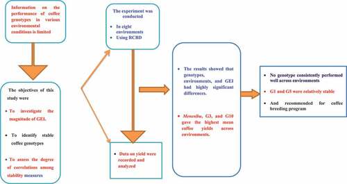
The performance of genotypes under diverse environments can be used to determine their adaptability and stability. However, information on the performance of coffee genotypes in various environmental conditions is limited. Thus, this study’s objectives were to estimate genotype by environment interaction (GEI), evaluate the mean performance and stability of 16 fruity flavored coffee genotypes in eight specialty coffee growing environments in western Ethiopia, and assess the magnitude of correlations among different stability parameters. The experiment was laid out in a randomized complete block design (RCBD) with two replications. For coffee yield, data were recorded and a combined analysis of variance and stability analysis were performed. Additive main effect and multiplicative interaction (AMMI) analysis revealed that genotypes, environments, and GEI showed highly significant differences (P < .0.01) for coffee bean yield. AMMI analysis also revealed that 73.2% of the GEI sum of squares for coffee bean yield was accounted for by the first three interaction principal component axes (IPCA). The standard check variety G16 (Menesibu), G3(W54/99), and G10 (W107/99) gave the highest average yields of 1537, 1458 and 1375 kg of clean coffee per hectare across environments, respectively. Despite no genotypes consistently performing well across environments due to the high GEI, G1 (W13/99) and G5 (W54/99) were relatively stable. Therefore, these were recommended as useful genetic resources for breeding of high-yielding genotypes. However, since all the genotypes gave a mean yield below the standard check variety, additional genotypes should be tested in more environments to develop stable and high-yielding coffee varieties.

Graphical abstract

KEYWORDS:

• AMMI
• Coffea arabica
• coffee bean yield
• GEI
• RCBD
• yield stability

1. Introduction

Coffee is one of the world’s most widely consumed beverages and a key source of foreign exchange for many developing countries. Coffea has three species used to make coffee: C. arabica, C. canephora, and C. liberica. Among the three, C. arabica is the most important commercial species (Coste, 1992).

The coffee business directly or indirectly sustains the livelihoods of around 20–25 million Ethiopians. According to CSA (Central statistical authority; 2017), the estimated area of land covered by coffee in Ethiopia is about 700, 474.69 ha. However, the national average yield of 0.646 t/ha (CSA (Central Statistical Agency), 2019) is lower than the global average yield of 0.791 t/ha (Boansi & Crentsil, 2013) and significantly lower than the potential average yields of 1.55 t/ha on farmer fields and 2.15 t/ha on research stations using improved varieties and production technologies such as optimal land preparation, weeding, fertilizer application, and so on (Kufa, 2018).

Ethiopia’s low average yield and quality of coffee have been attributed to the use of local landraces, traditional coffee husbandry, inefficient harvesting, and post-harvest handling practices (Kufa, 2010). A shortage of suitable cultivars with superior yield performance across varied growing situations is another bottleneck affecting Ethiopian coffee productivity.

Ethiopia’s agro-ecologies are diversified and suitable for coffee cultivation. Coffee is produced at altitudes ranging from 550 to 2,750 meters above sea level. However, the presence of genotype-by-environment interaction limits the development of high-yielding coffee cultivars with greater adaptability (Ameha & Belachew, 1987; Beksisa et al., 2018; Belete & Belachew, 2008; Belete et al., 2014). The varied response of crop genotypes to changing environmental conditions, known as genotype-by-environment interaction (GEI), makes selecting superior genotypes difficult and slows selection progress. Thus, evaluating a group of genotypes under different environmental conditions has become a crucial part of any breeding effort (Kumaresan & Nadarajan, 2010), as it helps to determine whether to develop cultivars for all environments or to develop specific cultivars for specific target environments.

Various statistical techniques have been applied to measure GEI and yield stability in crops. According to Ghaderi et al. (1980), the conventional analysis of variance approach is beneficial for determining the magnitude of GEI. Still, it does not provide additional information on the contribution of specific genotypes to GEI. As a result, various statistical approaches have been devised to address the issue. For instance, Wricke’s ecovalence (Wricke, 1962), the joint regression model (Eberhart & Russell, 1966), static stability coefficient (Becker & Leon, 1988; Lin et al., 1986), cultivar superiority measure (Lin & Binns, 1988), the AMMI model (Gauch & Zobel, 1988), AMMI stability value (Purchase, 1997), and yield stability index (Farshadfar et al., 2011).

There are three ways for cultivar suggestion and exploitation of the GEI in a crop breeding program, according to Eisemann et al. (1990):(1) Ignoring them, that is, using genotypic means across environments as a criterion for cultivar endorsement notwithstanding the presence of GEI. (2) Avoiding them: this entails decreasing the impact of GEI by comparable grouping environments and recommending cultivars that are specifically suited to each mega environment. (3) Exploiting them-the breeding program focuses on determining the stability of genotypic performance across diverse environments by examining and interpreting the influence of GEI on wide adaptation.

Despite the prevalence of genotype-environment interaction (GEI) on coffee bean yield, there is still a chance to develop high-yielding stable genotypes that have wider or specific adaptations as Ethiopia is endowed with enormous coffee genetic resources and diverse agro-ecologies suitable for coffee production. The previous investigators identified and recommended high-yielding and widely adapted genotypes for the winey flavored coffee-growing areas of southwestern Ethiopia using the parameters mentioned above (Beksisa et al., 2018; Tefera, 2017; Legesse, 2017; Merga, 2019). Besides, Legesse (2017) and Beksisa et al. (2018) also identified coffee genotypes as having specific adaptations. However, no information is available on GEI and stability in yield performance of fruity-flavored coffee genotypes from western Ethiopia. Therefore, the objectives of this study were to investigate the magnitude and pattern of GEI, to evaluate the mean yield performance, to identify stable and high yielding genotypes for broad and specific adaptation to enhance fruity flavored Arabica coffee productivity in Ethiopia’s specialty coffee growing environments of western Ethiopia, and to assess the degree of correlations among different stability parameters

2. Materials and methods

2.1. Experimental locations

The field experiments were conducted during 2015, 2016, and 2017 cropping seasons in eight environments, namely: Haru 2015, Nedjo 2015, Mugi 2015, Haru 2016, Nedjo 2016, Mugi 2016, Haru 2017, and Mugi 2017, which represent the major fruity-flavored coffee-growing areas of western Ethiopia. The number of interactions between the environment and the year would have been nine. Still, the third-year data of one environment, Nedjo 2017, was lost due to the frost problem, forcing the analysis to be made for data from eight environments. The study areas are shown in Figure 1, and Table 1 summarizes the characteristics of each testing environment.

Figure 1. Map of the study areas.

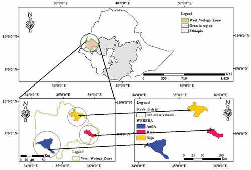
Table 1. Description of testing environments for testing 16 Arabica coffee genotypes.

Location	Year	Environment code	Alt. (masl)	Lati.	Longti.	Soil type	Temperature (^0c)			Rainfall (mm)
							Max.	Min.	Average
Haru	2015 2016 2017	E1 E4 E7	1752	08° 59’	35 ° 47’	Acrisol	26.50 25.67 26.30	-14.51 16.90	-20.09 21.60	1904 1654 1900
Nedjo	2015 2016	E2 E5	1753	09° 05’	35 ^0 45’	Nitosol	26.71 26.68	12.31 12.03	19.51 19.36	1864 1666
Mugi (Anfilo)	2015 2016 2017	E3 E6 E8	1570	08° 40’	34 ° 00’	Nitosol	30.40 30.90 31.10	15.90 16.90 16.20	23.15 23.90 23.65	1702 1690 1720

Note: – Alt. = altitude, Lati, = latitude, Longi = longitude, masl = meter above sea level, Max. = maximum and Min. = minimum

2.2. Experimental materials, design, and field management

The experiment was conducted on 16 coffee genotypes (Table 2). Twelve promising genotypes were chosen out of 88 genotypes from the earlier trial at Haru agricultural research sub-center based on their high yield, quality, disease resistance level, and morphological character variation. Hence, these 12 genotypes, together with four recently released varieties (Menesibu, Haru 1, Chala, and Sende) were used for the study. The field experiment was laid out in a randomized complete block design (RCBD) with two replications at each location. From each genotype, twelve coffee seedlings with six to eight pairs of true leaves, which have been grown in the nursery, were planted under uniform shade trees of Sesbania sesban in 2011 at a planting distance of 2 m x 2 m. The ten central coffee plants were used as experimental plants, whereas the two coffee plants on both sides of each plot were used as border plants to avoid the border effects. After planting, all the recommended agronomic practices such as hand weeding/slashing, pruning, fertilizer application, etc. were applied according to the recommendation for each location (Taye et al., 2008).

Table 2. List of coffee genotypes used in this study and their collection sites.

No	Genotypes	Altitude	Collection woreda	Specific location	Remark
1	W13/99	1650	Haru	Diritoli	Landraces
2	W18/99	1700	Haru	Diritoli	Landraces
3	W54/99	1700	Haru	Dogi Adere	Landraces
4	W74/99	1940	Haru	Keki	Landraces
5	W96/99	1600	Haru	Keki	Landraces
6	W98/99	1580	Haru	Keki	Landraces
7	W99/99	1580	Haru	Keki	Landraces
8	W102/99	1580	Haru	Keki	Landraces
9	W103/99	1580	Haru	Keki	Landraces
10	W107/99	1610	Haru	Keki	Landraces
11	W108/99	1670	Haru	Keki	Landraces
12	W110/99	1670	Haru	Keki	Landraces
13	Haru 1				Standard check
14	Chala				Standard check
15	Sinde				Standard check
16	Menesibu				Standard check

2.3. Data collected

Fresh cherries were picked and weighed in grams from each plot/genotype and then divided by the number of bearing trees. The gram per tree average fresh cherry yield was eventually converted to a kilogram of clean coffee yield per hectare (kg/ha).

2.4. Statistical analysis

2.4.1. Analysis of variance (ANOVA)

The assumptions of the analysis of variance (ANOVA): normality test and test of equal variance were performed for each environment using SAS statistical software (SAS, 2014), and there were no violations of these assumptions. Therefore, an analysis of variance was done for the eight environments separately to see if there was any difference among the genotypes for coffee bean yield. The yield data of each environment was analyzed using the following model:

(1) $Yij=\mu +Gi+Bj+\epsilon ij$(1)

Where: Yij is the observed value of i^th genotype in the j^th block, μ is the grand mean yield, Gi is the effect of the i^th

genotype, Bj is the effect of the j^th block, and Ɛij is the error (random) effect of i^th genotype in the j^th block

Before combining the data, Bartlett’s test (Steel & Torrie, 1998) was performed, and the test revealed that variances among the environments were heterogeneous for coffee yield. Therefore, coffee bean yield data were transformed using logarithm transformation according to Gomez and Gomez (1984). After transformation, the variance among environments became homogeneous. Then, the AMMI method, as described in Zobel et al. (1988), was used to analyze adaptability and phenotypic stability using the following statistical model

(2) $Y_{ij}=\mu +{\mathrm{G}}_{\mathrm{i}}+{\mathrm{E}}_{\mathrm{j}}+\sum _{n=1}^N{\lambda }_{\mathrm{n}}{\alpha }_{\mathrm{n}\mathrm{i}}.{\mathrm{Y}}_{\mathrm{n}\mathrm{j}}+{\mathrm{R}}_{\mathrm{i}\mathrm{j}}++{\epsilon }_{ij}$(2)

Where Y_ij is the yield of i^th genotype in j^th environment

• μ = the grand mean

• G_i = the mean of i^th genotype minus the grand mean (genotype deviation from the grand mean)

• Ej = the mean of j^th environment minus the grand mean (environment deviation from the grand mean

• N = the number of principal components retained for analyses

• λ_n= the square roots of the eigenvalue of n^th the principal component axis (PCA)

• α_ni = the principal component scores of n^thPCA axis of i^th genotype

• Y_nj= the principal component scores of n^th PCA axis of j^th environment

• R_ij = the residual and εij = random error term

2.4.2. Stability analysis

The AMMI stability value (ASV) of Purchase (1997) was calculated using Microsoft Office Excel 2007 to quantify and rank genotypes based on their yield stability.

(3) $\mathrm{A}\mathrm{S}{\mathrm{V}}_{\mathrm{i}}=\hspace{0.17em}(\frac{IPCA1ss}{IPCA2ss}i\ast \left(IPCA1score\right)i{]}^2+\left(IPCA2score\right)i2$(3)

Where: ASV_i is the AMMI stability value of i^th genotype

IPCA1ss is the sum of the squares of interaction principal component axis one of i^th genotype

IPCA2ss is the sum of the squares of interaction principal component axis two of i^th genotype

IPCA1 and IPCA2 scores are the values of interaction principal components axis one and two of the i^th genotype.

Besides, the cultivar superiority measure (Pi) was calculated by dividing the sum of squares of differences between genotypes yield and maximum yield at a given environment by twice the number of environments (Lin & Binns, 1988). Pi was generated with GenStat version17th software.

(4) ${\mathrm{P}}_{\mathrm{i}}=\frac{{\sum }_{\mathrm{j}=0}^{\mathrm{n}}{({\mathrm{Y}}_{\mathrm{i}\mathrm{j}}-{\mathrm{M}}_{\mathrm{j}})}^2}{2\mathrm{e}}$(4)

Where Y_ij = the yield of i^th genotype in the j^th environment, M_j = the genotype with maximum yield among all genotypes in the j^th environment, and e is the total number of environments.

The stability of each genotype was further estimated according to Wricke (1962) using GenStat version 17^th software (Roger et al., 2014). The stability of the i^th genotype (ecovalence (Wi) is its interaction with the environments, squared and summed across environments, and is stated as:

(5) $W_i=\sum _{j=0}^n{\left({\bar{Y}}_{ij}-{\bar{Y}}_i-{\bar{Y}}_j-\mu \right)}^2$(5)

Where: Ȳ_ij = the mean performance of i^th genotype in j^th environment

Ȳ_i = the mean performance of i^th genotype

Ȳ_j = the mean performance of j^th environment and

µ = the overall mean.

The approach known as YSI, which was developed by Farshadfar et al. (2011), was also performed to see the genotypes’ stability. YSI_i was calculated as:

(6) $YS{I}_i=RAS{V}_i+R{Y}_i$(6)

Where YSI_i = yield stability index of i^th genotype

RASVi is the i^th genotype rank in terms of AMMI stability value.

RYi is the rank of i^th genotype based on average yield across different environments

The static stability coefficient (SSC), the variance of yields of each genotype over test environments (Becker & Leon, 1988; Lin et al., 1986), was computed using GenStat version 17^th software using the following formula.

(7) $s_{Xi}^2=\frac{\sum {\left(X_{ij}-Y_I\right)}^2}{E-1}$(7)

Where X_ij is the bean yield of genotype i in environment j, Y_i. is the mean yield of genotype i, and E is the number of environments

Finally, Eberhart and Russell’s (1966) joint regression model was performed to see the stability of coffee genotypes for coffee bean yield. The analysis was performed using the SPAR 2 analytical software using the following model.

(8) $Y_{ij}={\mu }_i+{\beta }_{i.}{I}_j+S_{ij}$(8)

Where: Y_ij is the mean of the i^th genotype in the j^th environment, µ_i is the mean of the i^th genotype across all environments, β_i is the regression coefficient that measures the response of the i^th genotype to varying environments, I_j is the environmental index obtained as the mean of all genotypes in the j^th environment minus the grand mean and S_ij the regression deviation of the i^th genotype in the j^th environment

The two stability parameters, regression coefficient (βi) and variance of the regression deviation S²_di were estimated as

(9) ${\beta }_i=\frac{\mathrm{\Sigma }{Y}_{ij}{I}_j}{\mathrm{\Sigma }{I_j}^2}$(9)

Whereas the sum of the product of the i^th observation in the j^th environment with its environmental index, and is the sum of the squares of each environmental index. The deviations [= (y_ij – y _ij)] can be squared and summed to provide an estimate of another stability parameter

(10) $S_{di}^2=\frac{{\mathrm{\Sigma }}_j{{\sigma }_{ij}}^2}{n-2}-\frac{S^{2}e}{r}$(10)

where S²e/r is the estimate of the pooled error. The regression coefficient (βi) is tested for its significance from unity using the t-test, while the F-test tested the significance of the S²d_ij from zero by comparing deviations from regression with a pooled error estimate

2.4.3. Correlation between stability parameters

The Spearman rank correlation coefficients among stability parameters were calculated using the SAS statistical program (SAS, 2014) to compare the various stability parameters. Spearman correlation coefficient was calculated by using the following formula.

(11) $p=1-6\sum d{i}^2/n\left(n^2-1\right)$(11)

Where: P = Spearman’s rank correlation coefficient, d_i is the difference between the two ranks of each observation, and n is the number of observations

3. Results

3.1. Analysis of variance (ANOVA)

A separate ANOVA was computed for each location, and the mean coffee bean yield of 16 coffee genotypes is presented in Table 3. Genotypes showed significant variations in coffee bean yield in all environments except for E1, E5, and E7. Moreover, the combined analysis of variance using the AMMI model (Table 4) revealed that the main effects, as well as their interaction, showed highly significant (p < 0.01) differences in coffee bean yield. The proportion of the sum of squares for the environment was the largest source of variation (42.0%), followed by genotype by environment interaction (28.92%), error (18.77%), and genotype (6.78%). The AMMI analysis also revealed that the first three IPC axes were significant and explained 73.20% of the GEI. The first, second, and third IPCAs accounted for 29.77%, 26.43%, and 17.00% of the total interaction sum of squares, respectively.

Table 3. Mean clean coffee yield (kg/ha) of 16 tested coffee genotypes across eight environments.

Genotypes	Environmental codes
	E1	E2	E3	E4	E5	E 6	E7	E8	Genotypes mean
G1(W13/99)	865	532	1055	1248	600	1347	1929	2234	1226
G2(W18/99)	1260	826	761	863	743	1191	948	1381	997
G3(W54/99)	1009	605	1406	912	509	1637	1393	4189	1458
G4(W74/99)	866	412	1092	678	816	2370	2068	2172	1309
G5(W96/99)	758	556	1626	1310	374	1617	1748	2179	1271
G6(W98/99)	625	698	1044	1676	1221	1251	1572	1422	1189
G7(W99/99)	889	461	839	848	711	1280	936	1418	923
G8(W102/99)	1014	851	1615	513	872	2979	1606	1499	1368
G9(W103/99)	1352	599	716	925	558	727	1100	771	844
G10(W107/99)	522	537	1739	1397	754	2070	1130	2847	1375
G11(W108/99)	1109	296	695	1316	821	810	1081	1926	1007
G12(W110/99)	821	437	1418	1175	859	1399	742	1939	1099
G13(Haru 1)	686	390	622	1215	617	862	1196	1772	920
G14(Chala)	638	151	744	826	548	875	1334	2041	895
G15(Sinde)	1365	516	1021	519	1044	1612	689	2191	1120
G16(Menesibu)	1035	448	1061	951	975	2121	1129	4577	1537
Mean	926	520	1091	1023	751	1509	1288	2160	1159
F-test	NS	*	*	*	NS	**	NS	**
LSD	-	0.855	1.643	1.501	-	2.369	-	3.082

Note:- E1 = Haru 2015, E2 = Nedjo 2015, E3 = Mugi 2015, E4 = Haru 2016, E5 = Nedjo 2016, E6 = Mugi 2016, E7 = Haru 2017, E8 = Mugi 2017 and LSD = least significant difference. *, ** and NS are significant, highly significant, and non-significant, respectively

Table 4. ANOVA of AMMI model for clean coffee yield (kg/ha) of coffee genotypes across different environments during 2015, 2016, and 2017 cropping seasons.

Source of Variation	DF	SS	MS	% GEI variation explained	Cumulative	Total variation Explained
Total	255	18.43	0.07
Genotypes	15	1.263	0.08**			6.78
Environments	7	7.697	1.10**			42.00
Block	8	0.649	0.08**			3.53
Interactions	105	5.319	0.05**			28.92
IPCA 1	21	1.577	0.08**	29.77	29.77
IPCA 2	19	1.414	0.07**	26.43	56.20
IPCA 3	17	0.903	0.05*	17.0	73.20
IPCA 4	15	0.701	0.05^NS	13.18	86.38
Residuals	33	0.724	0.02	13.62	100.00
Error	120	3.403	0.03			18.77

Note:- DF = degrees of freedom, SS = sum of the squares, MS = mean of the squares, GEI = genotype by environment interaction, ** and * = statistically significant at 1 and 5% probability level, NS = non-significant, and IPCA = interaction principal component

3.2. Comparison of mean coffee bean yields

The largest environmental effect on coffee bean yield indicated that environments were diverse, with significant differences among environmental means. The mean coffee bean yield of the environments ranged from 520 kg/ha (E2 (Nedjo 2015) to 2160 kg/ha) E8 (Mugi 2017; Table 3). E1 (Haru 2015), E2 (Nedjo 2015), E3 (Mugi 2015), E4 (Haru 2016), and E5 (Nedjo 2016) yielded less than the grand mean yield of 1159 kg/ha. Only three environments, E6 (Mugi 2016), E7 (Haru 2017), and E8 (Mugi 2017), exceeded the grand mean yield (1159 kg/ha) with environmental mean yield values of 1509, 1288, and 2160 kg/ha, respectively

The mean coffee bean yield values of 16 coffee genotypes averaged over eight environments are presented in Table 3. The mean bean yield across eight environments ranged from 844 (G9) to 1537 kg/ha check variety (Menesibu), with a grand mean yield of 1159 kg/ha (Table 3). Eight genotypes, G16 (standard check variety Menesibu), G3(W54/99), G10 (W107/99), G8(W102/99), G4(W74/99), G5 (W96/99), G1(W13/99) and G6 (W98/99) gave mean yields of 1537, 1458, 1375, 1368, 1309, 1271, 1226, and 1189 kg/ha, respectively, above the grand mean yield of 1159 kg/ha. On the other hand, the other eight genotypes, including the three other standard check varieties, gave a mean yield below the grand mean of 1159 kg/ha. Accordingly, G15 (standard check variety Sende), G12 (W110/99), G11 (W108/99), G2 (W18/99), G7 (W99/99), G13 (standard check variety Haru 1), G14 (standard check variety Chala) and G9 (W103/99) gave mean yields of 1120, 1099, 1007, 997, 923, 920, 895, 844 kg/ha, respectively.

The strong GEI resulted in significant rank changes for some of the genotypes across the eight environments. For example, genotype G15 (Sende) was the highest yielding genotype in E1. However, it was one of the lowest-yielding genotypes, ranked 9^th, 10^th, 15^th, and 16^th at E2, E3, E4, and E7, respectively. G8 (W102/99) ranked first at E2 and E6, but 16^th and 12^th at E4 and E8. Similarly, G2(W18/99), G4 (W74/99), G6 (W98/99), G10 (W107/99), and G16 (Menesibu) also showed considerable rank changes across the testing environments.

3.3. Stability analysis for coffee bean yield

Different stability procedures were used to evaluate and describe the contribution of each coffee genotype to genotype by environment interaction and are presented in the following section.

AMMI biplot

The additive main effects and multiplicative interaction (AMMI) model is becoming a preferred statistical model for analyzing multi-environment yield trials, where there is GEI. This model combines analysis of variance (ANOVA) and principal component analysis (PCA; Gauch & Zobel, 1988), as well as estimating the contribution of each genotype and environment to total GEI variation (Hongyu et al., 2014). In the current study, the AMMI analysis revealed that the first two IPCAs alone accounted for 56.2% of GEI SS and were highly significant (P < 0.01; Table 4).

This analysis also provides a graphical representation (biplot) to summarize information on the main and interaction effects simultaneously (Crossa, 1990; Crossa et al., 1990). In the AMMI I biplot, the main effects (means of genotypes and environments) were represented by the abscissa (X-axis), and the first IPCA was used as the ordinate (Y-axis). Genotypes or environments located on the right-hand side of the midpoint of the axis main effects have higher yields than those on the left-hand side, with the midpoint representing the grand mean yield. In this biplot, the usual interpretation is that the displacements along the abscissa indicate differences in main effects, whereas displacements along the ordinate indicate differences in interaction effects. Similarly, the higher the IPCA I score, whether positive or negative, in AMMI I biplots, the more specifically adapted a genotype is to a specific environment, while the genotype is more stable across environments if the IPCA score is close to zero (Purchase, 1997; Wakjira & Labuschagne, 2002). On the other hand, in the AMMI II biplot, the first IPCA was used as the abscissa (X-axis), and the second IPCA was used as the ordinate (Y-axis). In this biplot, the genotypes and environments that are closer to the biplot’s center are more stable, and vice versa for the genotypes and environments that are more unstable (Purchase et al., 2000).

AMMMI biplots help to visualize genotypes that have wider or specific adaptations. Figure 2 shows the AMMI-I biplot for coffee bean yield of 16 genotypes in eight environments. In the current study, four groups of genotypes were identified from this biplot. The first group included seven genotypes, G1(W13/99), G3(W54/99), G4(W74/99), G5 (W96/99), G6 (W98/99), G8 (W102/99), and G16 (Menesibu) with mean coffee bean yield of more than the average and IPCA1 scores relatively closer to the point of origin. The second group had only one genotype, G10 (W107/99, with a mean coffee bean yield exceeding the average but a high IPCA-1 score of 0.37. The third group was composed of four genotypes, namely, G2 (W18/99), G9 (W103/99), G14 (Chala), and G15 (Sinde), which had mean coffee bean yields well below the average and high IPCA scores. The fourth group comprised four genotypes with low IPCA scores, G7 (W99/99), G11 (W108/99), G12 (W110/99), and G13 (Haru 1). However, none of these genotypes produced a yield that was significantly higher than the mean coffee bean yield. In general, the seven genotypes categorized under the first group are considered stable based on this model. The eight genotypes categorized under the third and fourth groups and one genotype in the second group, on the other hand, were unstable as the stable genotypes must show above the overall mean yield and low IPCA scores. Similarly, Figure 3 shows the AMMI-II biplot for coffee bean yield of 16 coffee genotypes in eight environments. The biplot revealed that G1 (W13/99), G3 (W54/99), G5 (W96/99), G6 (W98/99), G7 (W99/99), G12 (W110/99), G13 (Haru 1), and G16 (Menesibu) were stable genotypes as they were plotted relatively near to the origin in the biplot. However, genotypes must have a high yield above the grand mean to be considered stable, and therefore, genotypes G1 (W13/99), G3 (W54/99), G5 (W96/99), G6 (W98/99), and G16 (Menesibu) had mean yield above the grand mean and are stable. On the other hand, genotypes G2 (W18/99), G4 (74/99), G8 (W102/99), G9 (W103/99), G10 (W107/99), G11 (W08/99), G14 (Chala), and G15 (Sinde) were interactive as they were plotted far from the origin in the biplot, and these genotypes have specific adaptation (Figure 3).

Figure 2. AMMI 1 biplot showing genotype and environment means of coffee bean yield against IPC1.

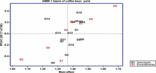
Figure 3. The AMMI II biplot showing the relationship between genotypes and environments for coffee mean yield.

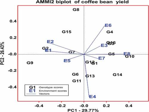
Aside from grouping genotypes, the biplots also group environments in discriminating the genotypes. In general, the testing environments showed variation in coffee bean yield, and the biplot showed that the points for the environment were more dispersed than the points for genotypes, implying that variability related to environments was greater than variability owing to genotypes. The AMMI I biplot revealed that E8 (Mugi 2017), E6 (Mugi 2016), and E7 (Haru 2017) were high yielding, while E1 (Haru 2015), E2 (Nedjo 2015), E3 (Mugi 2015), E4 (Haru 2016) and E5 (Nedjo 2016) gave mean bean yields below the grand mean and were the low yielding environments. In the biplot, among the eight testing environments, E1, E2, and E8 showed IPCA values distant from the origin, indicating that these environments discriminate the genotypes. On the other hand, the other five environments, E3, E4, E5, E6, and E7, had relatively low IPCA scores, and these environments were the least discriminating (Figure 2). On the other hand, the AMMI-II biplot revealed that only E3 (Mugi 2015), E5 (Nedjo 2016), and E7 (Haru 2017) were the most stable among the eight testing environments, as evidenced by values near the biplot’s origin, which imply a lesser contribution to GEI. The other five environments, E1 (Haru 2015), E2 (Nedjo 2015), E4 (Haru 2016/), E6 (Mugi 2016), and E8 (Mugi 2017), were the most unstable since they were far from the biplot’s origin, indicating that they contributed more to GEI (Figure 3).

Moreover, the sign of IPCA 1 for the genotypes and environments in the biplot also has important information on GEI. When genotype and environment have the same sign (positive or negative) on the IPCA1 axis, their interaction is positive, and if different, their interaction is negative. With the present data set, genotypes with positive IPCA1 scores, G1, G3, G4, G5, G10, G12, G13, G14, and G16 responded positively to the environments E3, E4, E6, E7, and E8 that had positive IPCA1 scores but negatively to the environments E1, E2, and E5 that had negative IPCA1. Similarly, genotypes with negative IPCA1 values, G2, G6, G7, G8, G9, G11, and G15 responded positively to environments E1, E2, and E5 that had negative IPCA1 scores but responded negatively to environments that had positive IPCA 1 values (Figure 2). The biplot also helps to appreciate environmental and genotype similarity for GEI and allows for the graphical estimation of these effects. In particular, the closeness between pairs of environments or pairs of genotypes in the biplot is proportional to their similarity in GEI effects. For example, G3 and G16 exerted similar effects for GEI or tend to have similar yields in all environments, whilst G3 exerted dissimilar effects with G14 or these two genotypes show different patterns of response over the environments as they were far apart. Likewise, E1 and E2 had almost similar effects for GEI, or these environments were found to have similar interaction patterns on the genotypes, whereas EI or E2 had dissimilar effects for GEI with E4, E6, and E8 (Figure 3)

AMMI stability value (ASV)

The ASV measure was proposed by Purchase et al. (2000) to cope with the fact that the AMMI model does not make a provision for a quantitative stability measure, and this value is finally used to measure the yield stability of the genotypes and cluster the genotypes and environments into different groups. Even if both IPCA1 and IPCA2 are helpful for stability indication, variation was observed in measuring the stable genotypes between the two IPCAs. That means a genotype considered stable in IPCA1 may not show itself stable in IPCA2 as in the first case. ASV values were calculated for each genotype, and the larger the ASV value, either negative or positive, the more specifically adapted a genotype is to certain environments. Conversely, lower ASV values indicate greater stability in different environments (Purchase et al., 2000)

Among the tested genotypes, G12 (W110/99), G1 (W13/99), G7 (W99/99), G5 (W96/99), G16 (Menesibu), and G3 (W54/99) showed relatively lower AMMI stability value (ASV) or higher stability. Nonetheless, better stability should not be used as the only criterion for genotype selection, as stable genotypes do not always result in higher yields (Mohammadi et al., 2007). Therefore, out of the six best genotypes with lower ASV, only four genotypes, G1, G3, G5, and G16, gave a mean coffee bean yield above the grand mean and were considered stable. However, although stable, G12 (W110/99) and G7 (W99/99) showed consistently low coffee bean yields across the testing environments. G4 (W74/99), G6 (W98/99), G8 (W102/99), and G10 (W107/99), on the other hand, were recognized as suitable genotypes to validate yield performance and particular adaptation since they showed higher ASV, i.e. low stability but mean bean yield above the grand mean. G2 (W18/99), G9 (W103/99), G11 (W108/99), G13 (Haru 1), G14 (Chala), and G15 (Sinde) all had mean yields below the grand mean and a high ASV, indicating low stability. (Table 5).

Table 5. The rank of 16 coffee genotypes based on mean yield, ASV, Cultivar Superiority Index (PI), Wricks’ecovalence (wi),YSI, and SSC.

Genotype	Mean yield			ASV		Pi		Wi		YSI		SSC		βi		S^2di
	Untrd	Transd	Rank	Transd.	Rank	Transd.	Rank	Transd.	Rank	Transd	Rank	Transd.	Rank	Transd.	Rank	Transd.	Rank
G1(W13/99)	1226	3.088	7	0.13417	2	0.02442	5	0.0481	2	9	3	0.04898	9	1.0776 ^ns	4	−0.0061^ns	8
G2(W18/99)	996	2.998	12	0.409054	14	0.04724	11	0.0928	6	26	11	0.01378	1	0.3447**	15	−0.0070 ^ns	10
G3(W54/99)	1458	3.164	2	0.261193	6	0.01648	2	0.0945	7	8	2	0.08355	14	1.4437**	10	−0.0002 ^ns	1
G4(W74/99)	1310	3.117	5	0.347246	10	0.02529	6	0.1300	12	15	6	0.06777	12	1.4781*	11	0.0041 ^ns	5
G5(W96/99)	1271	3.104	6	0.231643	4	0.02360	4	0.0915	5	10	4	0.05892	11	1.2363^ns	6	0.0098 ^ns	12
G6(W98/99)	1189	3.075	8	0.275537	8	0.03157	7	0.1054	9	16	7	0.01934	3	0.4899**	12	0.0046 ^ns	6
G7(W99/99)	923	2.965	13	0.150233	3	0.05048	13	0.0164	1	16	7	0.02391	4	0.7660**	7	−0.0142 ^ns	13
G8(W102/99)	1368	3.136	4	0.559148	15	0.03319	8	0.2650	16	19	8	0.05583	10	0.7395^ns	8	0.0326 ^ns	16
G9(W103/99)	844	2.926	16	0.561482	16	0.08375	16	0.2491	15	32	13	0.01509	2	0.1299**	16	0.0046 ^ns	7
G10(W107/99)	1375	3.138	3	0.394665	13	0.02282	3	0.1621	13	16	7	0.07487	13	1.3544 ^ns	9	0.0172 ^ns	15
G11(W108/99)	1007	3.003	11	0.350337	11	0.05031	12	0.1042	8	22	10	0.03303	5	0.9688^ns	1	0.0087 ^ns	11
G12(W110/99)	1099	3.041	10	0.100206	1	0.03591	9	0.0818	4	11	5	0.03515	6	0.9650 ^ns	2	0.0005 ^ns	2
G13(Haru 1)	920	2.964	14	0.271405	7	0.06018	14	0.0697	3	21	9	0.04837	8	0.9649 ^ns	3	−0.0032 ^ns	4
G14(Chala)	895	2.952	15	0.375571	12	0.07485	15	0.1258	10	27	12	0.08825	16	1.6325**	14	0.0062 ^ns	9
G15(Sinde)	1120	3.049	9	0.347113	9	0.04430	10	0.1866	14	18	8	0.04571	7	0.8581^ns	5	0.0157 ^ns	14
G16(Menesibu)	1537	3.187	1	0.255901	5	0.01585	1	0.1272	11	6	1	0.08412	15	1.5505**	13	−0.0029 ^ns	3
Mean	1159	3.057

Note: Untrd = untransformed (Original) and Transd. = transformed, Note = ** and * = statistically significant at 1 and 5% probability level, NS = non-significant. MY = mean yield, ASV = AMMI stability value, YSI = yield stability index, Pi = cultivar superiority index, Wi = Wricke’s (1962) ecovalence, SSC = static stability coefficient; β_i= regression coefficient and S²di = deviation from the regression

Cultivar superiority measure (Lin & Binns, 1988)

According to Lin and Binns (1988), the genotype with the lowest or smallest Pi value is the most stable. Accordingly, among the 16 genotypes evaluated in eight environments in the current study, the standard check variety G16 (Menesibu), G3 (54/99), G10 (107/99), G5 (96/99), and G1 (13/99) were the five relatively stable genotypes in this stability parameter. Furthermore, these genotypes exhibited a mean yield higher than the grand mean, making them the most stable genotypes. On the other hand, despite having greater mean yields than the grand mean, the three genotypes G6 (98/99), G8 (102/99), and G4 (74/99) were unstable, as evidenced by relatively higher Pi values. Similarly, the remaining eight genotypes all had lower mean coffee bean yields and higher Pi values and were not stable (Table 5).

Wricke’s ecovalence analysis (Wi)

According to Wricke (1962), the genotypes with the lowest ecovalence values were considered more stable than others. Therefore, based on this concept, Wricke’s ecovalence analysis identified the five best stable genotypes vis., G7 (99/99), G1 (13.99), G13 (Haru1), G12 (110/99), and G5 (96/99), which ranked first, second, third, fourth, and fifth, respectively. However, out of these five genotypes, only two genotypes, G5 (96/99) and G1 (13/99), gave mean yields above the grand mean and were stable. Besides, genotypes G7 (99/99), G13 (Haru 1), and G12 (W110/99), which showed low Wi values, were considered to be unstable as they gave mean coffee yields below the grand mean. This stability measure generally identified most high-yielding genotypes as unstable, whereas a few low-yielding genotypes as stable. For example, the high-yielding genotypes, G3 (54/99), G4 (W74/99), G6 (98/99), G8 (W102/99), G10 (W107/99), and G16 (Menesibu) ranked 7^th, 12^th, 9^th, 16^th, 13^th, and 11^th, respectively, based on their stability performance (Table 5).

Yield stability index

High-yielding genotypes are not always stable, and highly stable genotypes do not always have the best yield performance (Oliveira & Godoy, 2006). Therefore, keeping these points in view, the yield stability index (YSI) was proposed by Farshadfar et al. (2011). In this method, ASV was considered along with IPCA1 and IPCA2 for generating variation in the GE interaction. As a result, the lowest ASV takes the rank one. On the other hand, the highest average yield takes rank one, and then the ranks are added to a single simultaneous selection index of yield and stability named the yield stability index (YSI). The genotypes with low YSI would be considered high-yielding and stable. The YSI technique, which combines yield and stability into a single index, eliminates the difficulty of selecting varieties solely based on yield and has been effectively employed in other crops, such as wheat (Farshadfar et al., 2011). In this study, YSI identified four stable genotypes, namely, G16 (Menesibu), G3 (54/99), G1 (13/99), and G5 (96/99), with YSI values of 6, 8, 9, and 10, respectively. On the other hand, G11, G2, G14, and G9 were the least stable genotypes, with YSI values of 22, 26, 27, and 32, respectively. The other eight genotypes, G12, G4, G6, G7, G10, G8, G15, and G13, had medium stability with YSI values of 11, 15, 16, 16, 16, 19, 18, and 21, respectively (Table 5).

Static stability coefficient

Static stability coefficient (SSC) measures genotype performance consistency based on environmental variances, i.e. the variance of yields of each genotype across test environments (Lin et al., 1986). The static stability coefficient has a low value (near zero) when a genotype fits the static stability notion better. Therefore, the results of the current study based on this measure revealed that G2(18/99), G9(103/99), G6(98/99), G7(99/99), and G11 (Haru1) were stable genotypes but ranked 12^th,16^th, 8^th, 13^th, and 11^th for coffee mean yield, respectively (Table 5). Similarly, the five highest-yielding genotypes, G16 (Menesibu), G3 (54/99), G10 (107/99), G8 (102/99), and G4(74/99), ranked 15^th, 14^th, 13^th, 10^th, and 12^th for this stability measure, respectively. Therefore, this stability measure is ineffective for identifying high-yielding and stable genotypes

Joint regression analysis

The results of a joint regression analysis of coffee bean yield are shown in Table 6. The results demonstrated that there was a significant difference for genotypes (P < 0.05) and a highly significant difference for genotype x environment interaction (P < 0.01) (linear). Non-linear genotype by environment interactions, on the other hand, did not show any significant difference (P > 0.05) for coffee bean yield.

Table 6. Joint regression analysis of variance for coffee bean yield.

Source of variation	DF	SS	MS	V.R
Total	127	7.1695
Genotypes	15	0.6287	0.0419	2.044*
Env. + (genotypes X Env.)	112	6.5408
Environment (linear)	1	3.8712
Genotypes X Env. (linear)	15	0.7038	0.0469	2.913 **
Pooled Deviation	96	1.9657	0.0205	1.274^NS
G1(W13/99)	6	0.0600	0.0100	0.6211
G2(W18/99)	6	0.0543	0.0091	0.5652
G3(W54/99)	6	0.0952	0.0159	0.9876
G4(W74/99)	6	0.1209	0.0202	1.2547
G5(W96/99)	6	0.1551	0.0259	1.6087
G6(W98/99)	6	0.1239	0.0207	1.2857
G7(W99/99)	6	0.0112	0.0019	0.1180
G8(W102/99)	6	0.2921	0.0487	3.0248**
G9(W103/99)	6	0.1238	0.0206	1.2795
G10(W107/99)	6	0.1999	0.0333	2.0683
G11(W108/99)	6	0.1486	0.0248	1.5404
G12(W110/99)	6	0.0997	0.0166	1.0311
G13(Haru 1)	6	0.0772	0.0129	0.8012
G14(Chala)	6	0.1339	0.0223	1.3851
G15(Sinde)	6	0.1907	0.0318	1.9752
G16(Menesibu)	6	0.0792	0.0132	0.8199
Pooled Error	128	2.0574	0.0161

Note:- DF = degrees of freedom, SS = sum of the squares, MS = mean of the squares, V.R = variance ratio, ** and * = statistically significant at 1 and 5% probability level, NS = non-significant.

As a result, while determining the phenotypic stability of a genotype, the linear and non-linear (S²di) components of GEI were taken into account. The regression coefficient (β_i) and squared deviation (S²di) from the regression values are presented in Table 5. According to Eberhart and Russell (1966), the genotype is adapted to all environments if the regression coefficient is not significantly different from unity (βi = 1.0). Genotypes with β_i >1.0 are more responsive or adapted to high-yielding environments, whereas any genotype with β_i substantially lower than one (β_i<1) is adapted to low-yielding environments. Accordingly, G1, G5, G8, G10, G11, G12, G13, and G15 had nearly a unit (βi = 1.0) regression coefficient. The regression coefficients for G3, G4, G14, and G16 were significantly greater than one (β_i>1). On the other hand, G2, G6, G7, and G9 had regression coefficients of less than one (β_i<1). Moreover, deviation from the regression (S²di) is very important for understanding the stability of the genotypes. In the current study, all genotypes had a non-significant deviation from the regression.

According to Eberhart and Russell (1966), stable genotypes should have a non-significant value of S²di from zero, with a non-significant β_i value from unity and a higher mean yield above the average mean yield of genotypes. Therefore, four genotypes, G1, G5, G8, and G10 had a mean yield above the grand mean, a non-significant deviation of regression coefficients from unity, and a non-significant deviation of S²di values from zero and, therefore, are desirable genotypes for growing in all environments. On the other hand, despite the four genotypes, G11, G12, G13, and G15, having a non-significant deviation of regression coefficients from unity and a non-significant variation of S²d values from zero, they had a mean yield lower than the grand mean. Therefore, these genotypes are not suitable for all environments. The other three genotypes, G3, G4, and G16, had regression coefficients significantly greater than one (β_i1 > 1), non-significant deviation of S²di values from zero, and a high mean yield, above-average yield of genotypes, which suggested that these genotypes were suitable for favorable environments. Similarly, G2, G7, and G9 had regression coefficients significantly lower than one (β_i<1) and a non-significant deviation of S²di values from zero and a lower mean yield, suggesting these genotypes were suitable for unfavorable environments.

3.4. Correlation between different stability parameters

Table 7 shows Spearman’s rank correlation coefficients among the different stability measures. The results showed that positive and highly significant correlations (P < 0.01) were observed between the ranks of mean coffee yield (MY) and cultivar superiority index (Pi) (r = 0.955), mean yield (MY), and yield stability index (YSI) (r = 0.792), AMMI stability value (ASV) and Wricks ecovalence(Wi) (r = 0.741), AMMI stability value (ASV) and yield stability index (YSI) (r = 0.732) and the cultivar superiority index (Pi) and yield stability index (YSI) (r = 0.872). Similarly, a significant correlation was observed between the rank of ASV and the regression coefficient (β_i)(r = 0.524) (P < 0.05).On the other hand, negative and significant correlations (p < 0.05) were observed between the ranks of mean yield (MY) and static stability coefficient (SSC (r = −0.573), and cultivar superiority index (Pi) and static stability coefficient (SSC) (r = −0.523). However, the correlations between most of the other pairs of stability measures were weak (Table 7)

Table 7. The Spearman’s rank correlation of different stability measures of coffee bean yield.

	MY	ASV	Pi	WI	YSI	SSC	βi	S^2di
MY	0	0.191^NS	0.955**	0.238 ^NS	0.792**	−0.573*	0.018^NS	0.053 ^NS
ASV		0	0.350 ^NS	0.741**	0.732 **	−0.124 ^NS	0.524*	0.406 ^NS
Pi			0	−0.0471 ^NS	0.872**	−0.523 *	−0.018 ^NS	0.159 ^NS
Wi	-			0	0.287 ^NS	0.194 ^NS	0.447 ^NS	0.285 ^NS
YSI					0	−0.471 ^NS	0.219 ^NS	0.372 ^NS
SSC						0	0.062 ^NS	−0.126 ^NS
bi							0	−0.109 ^NS
sid								0

Note: = ** and * = statistically significant at 1 and 5% probability level, NS = non-significant. MY = mean yield, ASV = AMMI stability value, YSI = yield stability index, Pi = cultivar superiority index, Wi = Wricke’s (1962) ecovalence, SSC = static stability coefficient; β_i= regression coefficient and S²di = deviation from the regression

4. Discussion

4.1. Analysis of variance (ANOVA)

The current study assessed genotype by environment interaction and stability performance of 16 coffee genotypes in eight Wollega specialty coffee growing environments.

Individual environment analysis revealed significant variation among the genotypes for coffee bean yield in most environments. The significant variation indicates the existence of variability among the genotypes and, thus, is important for further breeding purposes to develop varieties with wide and specific adaptation. A similar result has been reported by Belete et al. (2014), who studied the yield performance of 30 Arabica coffee genotypes in eight environments. Moreover, the combined analysis of variance using the additive main effect and multiplicative interaction (AMMI) model revealed that coffee bean yield was significantly affected by genotype, environment, and GEI. The variation among genotypes in the different environments and significant GEI for coffee bean yield implies that identifying a superior genotype doing well across all the environments may be difficult, as a genotype with the best performance in one environment may not do well in the other. The GEI illustrates a fundamental idea: even if all plants were genetically identical (the same genotype), they wouldn’t always display their genetic potential in the same manner under diverse environmental conditions.

Similarly, considerable differences among environments suggest that the testing environments differed in biotic (pest occurrence) and abiotic factors (edaphic and climatic variables). Moreover, the significant influence of the environment was demonstrated by its impact on coffee bean yield. Earlier reports in Ethiopia have also shown that the environment was the major source of the total variation in coffee bean yield (Beksisa et al., 2018; Legesse, 2017; Walyaro, 1983). The result of AMMI analysis also revealed that the first three IPC axes were significant and explained 73.20% of the GEI. The first two IPCA scores were highly significant (P < 0.01) and cumulatively accounted for 56.20% of the total GEI sum square, indicating the capability of the first two principal component axes for cross-validation of variations explained by GEI (Zobel et al., 1988). The values explained by the model in this study were comparable with the previous findings of Beksisa et al. (2018), who reported that the first two IPCAs accounted for 63.21% of the total GEI sum square

4.2. Comparison of mean coffee bean yields

The mean coffee bean yield across environments ranged from 520 kg/ha (E2) to 2160 kg/ha (E8). The yields recorded at E1, E2, E3, E4, and E5 were less than the grand mean yield (1159 kg/ha), which was, however, surpassed by only three environments, E6, E7, and E8. This difference could be attributed to the variation in climatic factors and soil conditions of the environments during the growing seasons. The optimum temperature for coffee plant physiological process vary with age and Mamo et al. (2008) reported that a temperature of about 22–25°C and total annual rainfall of greater than 1300 mm is optimum or highly suitable for mature coffee tree. Apart from average annual temperature and the total annual rainfall, the condition of the soils especially the PH that affect the nutrient availability is also an important factor for high coffee bean yield, and the optimum soil PH is 5.8.-6.0 (Wrigley, 1988). Therefore, the highest yields recorded in Mugi environments, E6 and E8 (Table 3), could be mainly due to the optimum annual average temperature of these environments (Table 1). On the other hand, the low average annual temperature (Table 1) might have contributed to the low coffee bean yields in Nedjo environments (E2 and E5; Table 3). Besides, the soils of Nedjo are confirmed to be highly acidic with pH of 4.4 (Agegnehu, 2020; Hirpa et al., 2013) and according to the authors, soil acidity converts available soil nutrients into unavailable forms, and soils affected by soil acidity are poor in their basic cations that are essential to crop growth and development. Hence, the poor or low yield in Nedjo environments could be attributed to the low PH or highly acidic nature of the soils. In agreement with the current results, Legesse (2017) and Tefera (2017) have reported significant variation among environments for coffee bean yield.

The mean yield of coffee genotypes over the eight environments ranged from 844 kg/ha (G9) to 1537 kg/ha (standard check variety, Menesibu), with a grand mean of 1159 kg/ha. Eight genotypes gave a mean yield above the grand mean. In general, genotypes G3 (W54/99), G10 (W107/99), G8 (W102/99), G4 (W74/99), G5 (W96/99), G1 (W13/99), and G6 (W98/99) exhibited yield advantages over the three standard check varieties (Haru 1, Chala, and Sende), though lower than the yields of the best standard check variety, Menesibu. Therefore, these genotypes could be considered for western Ethiopia’s future coffee variety improvement program.

In the current study, the performance of the genotypes across the eight environments was not consistent due to the high GEI effects which resulted in significant rank changes. For example, genotype G15 (Sende) was the highest yielding genotype in E1. However, it was one of the lowest-yielding genotypes, ranked 9^th, 10^th, 15^th, and 16^th at E2, E3, E4, and E7, respectively. G8 (W102/99) ranked first at E2 and E6, but 16^th and 12^th at E4 and E8. Similarly, G2(W18/99), G4 (W74/99), G6 (W98/99), G10 (W107/99), and G16 (Menesibu) also showed considerable rank changes across the testing environments. This indicates that no genotype performed best in all environments as the genotypes exhibited different levels of phenotypic expression under different environmental conditions because yield is a quantitative trait controlled by many genes and affected by the environment to varying degrees. Hence, GEI in the current study results from variations in genotypes’ sensitivity to various environmental variables (soil condition, temperature, disease pressure, etc.). According to Robertson (1959), the diverse reactions of genotypes to different environments result from the expression of different gene sets in different environments as well as differences in responses to the same set of genes in other situations. In agreement with the current findings, Walyaro (1983), Ameha and Belachew (1987), and Belete et al. (2014) have reported considerable differences among coffee genotypes due to significant GEI for coffee bean yield. Therefore, the existence of GEI for coffee bean yield indicates the need to identify high-yielding and stable genotypes across locations or select genotypes for specific adaptation.

4.3. Stability analysis for coffee bean yield

In the present study, AMMI biplots identified five stable and high-yielding genotypes (G1, G3, G5, G6, and G16). Similarly, AMMI Stability Value (ASV), cultivar superiority measure (Pi), and yield stability index (YSI) identified four genotypes, G1 (13/99), G3(54/99), G5(96/99), and G16(Menesibu) as high-yielding and stable. On the other hand, results of joint regression analysis identified four (G1, G5, G8, and G10) and Wricks ecovalence (Wi), two (G1 and G5) high-yielding and stable genotypes. In general, despite the inconsistency among stability parameters, all identified two high-yielding and stable genotypes (G1 and G5) in common, and thus, these genotypes can be used as useful genetic resources to improve coffee bean yield . This implies that applying such modern stability parameters will help improve selection accuracy and identify genotypes that combine high yield and stability. In line with this, these stability parameters have been successfully used to identify stable genotypes in different crops, including coffee (Demesse et al., 2011; Tefera, 2017); hybrid rose (Yousefi et al., 2011); sesame(Belay, 2016), and grain sorghum (Al-Naggar et al., 2018). Apart from identifying widely adapted genotypes, the AMMI biplots and the majority of the other stability parameters identified four genotypes: G4 (74/99), G6 (98/99), G8 (102/99), and G10 (107/99), which are high yielders but highly interactive, indicating that these genotypes are extremely sensitive to the environment. As a result, they may be used in specific environments. In addition to identifying stable genotypes, the AMMI biplots identified the three stable/favorable environments (E3, E5, and E7) that can be used for widely adapted genotypes and five interactive environments (E1, E2, E4, E6, and E8) that can be used for genotypes with specific adaptations. This result was in agreement with the findings of Legesse (2017) and Beksisa et al. (2018), who identified environments that can be used for broadly and specifically adapting genotypes.

Partitioning of genotype x environment interaction by joint regression analysis revealed a highly significant difference, indicating that the linear component contributed a considerable proportion of the genotype x environment interaction (Table 7). Therefore, prediction for most of the genotypes appeared feasible for yield. However, non-significant mean squares due to pooled deviation for yield revealed that a non-linear component is less critical in accounting for the total genotype x environment interaction. In the current study, all the three parameters of stability, i.e. mean coffee yield, regression coefficient, and standard deviation to regression, provided clear evidence that G1, G5, G8, and G10 were suitable for general adaptation and, thus, could be grown in all environments. Conversely, G11, G12, G13, and G15 gave lower bean yields, below the average, and had regression coefficients closer to one (β_i = 1) and squared deviations from regressions closer to zero (S² di = 0) and, hence, are poorly adapted to all environments.

On the other hand, G3, G4, and G16 had regression coefficients significantly greater than one (β_i>1), non-significant deviation of S²di values from zero and high mean yields suggesting that these genotypes tend to respond favorably to better environments but give poor yield in unfavorable environments. In line with this, Eberhart and Russell (1966) reported that such genotypes are suitable for favorable environments. On the other hand, three genotypes, G2, G7, and G9, had regression coefficient values significantly less than one (βi<1), non-significant deviation from regression (S²di<0), and mean yield below the average, indicating that these genotypes are stable and well adapted to unfavorable environments. Therefore, this study showed that coffee genotypes differed considerably in yield stability. Fikadu Tefera (2017) and Beksisa et al. (2018) have reported similar results using different stability parameters for coffee.

4.4. Correlation between different stability parameters

Spearman’s coefficient of rank correlation was computed for all the stability parameters together with the mean bean yield. It was observed that the two stability measures, cultivar superiority measure (Pi) and yield stability index (YSI), which had significant positive associations with each other, also showed strong positive rank correlations with mean coffee bean yield. Hence, these statistics are related to the dynamic concept of stability, and selection based on each is acceptable (Becker & Leon, 1988). This result indicates that the use of Pi and YSI as a tool to evaluate the stability of coffee genotypes would favor the section of high-yielding and stable coffee genotypes. Similarly, the positive and significant association of AMMI stability value (ASV) with Wricks ecovalence (Wi), yield stability index (YSI), and regression coefficient (β_i) indicates that ASV was similar to these three measures in evaluating the stability performance of coffee genotypes. Hence, due to its simplicity and strong positive correlation with the above stability measures, ASV can also be the best measure for classifying coffee genotypes based on their stability under different environmental conditions.

On the other hand, the significant negative rank correlation between mean yield (MY) and static stability coefficient (SSC) suggests that selection based on this stability parameter would be less useful when yield is the primary target of selection. The positive and significant association observed between mean yield ranking and Pi in this study was in agreement with the findings of Karimizadeh et al. (2012) in Lenti; Belay (2016) in sesame; and Beksisa et al. (2018) in coffee. Likewise, the positive and significant correlation of YSI with mean yield, Pi, and ASV ranking was similar to the findings of Legesse (2017). However, the significant association observed between Wi and ASV does not agree with the finding of Legesse (2017), who reported a non-significant correlation. This variation might have been attributed to the variation in study materials and testing sites. The negative and significant correlations observed between Pi-SSC, on the other hand, imply that these pairs of stability measures rank genotypes in the opposite order; for example, G16 ranks first in Pi but 15^th in static stability measure. In agreement with the present observation, Beksisa et al. (2018) have reported a negative and non-significant correlation between MY-SSC, Pi-Wi, and SSC-YSI in coffee.

5. Conclusion

The results showed that genotype, environment, and GEI significantly influenced coffee yield. The study also confirmed that the standard check variety G16 (Menesibu), G3 (W54/99), and G10 (W107/99) gave the highest average coffee yield across environments. Similarly, higher yields were observed at E6 (Mugi 2016) and E8 (Mugi 2017). Despite no genotypes consistently performing well across environments due to the high GEI, genotypes, G1 (W13/99) and G5 (W54/99) were relatively stable. Therefore, these were recommended as useful genetic resources for breeding of high-yielding coffee genotypes under western Ethiopia or similar environments. Moreover, genotypes having a mean yield above the grand mean (for example, G4, G6, G8, and G10) can be used for specific and favorable environments. The study has generally proved that the AMMI, Pi, YSI, ASV, and Eberhart and Russell joint regression models are important to study the stability of coffee genotypes. However, the strong rank correlations observed between ASV and most of the stability measures indicated close similarity and effectiveness in studying the stability analysis. Therefore, ASV can be used to identify stable coffee genotypes. However, all the tested genotypes in the current gave lower yields than the standard check variety (Menesibu). Therefore, to get high-yielding and stable genotypes, it is suggested to conduct a further study by including additional genotypes and testing locations in western Ethiopia.

Acknowledgments

The authors would like to thank the Ethiopian Institute of Agricultural Research (EIAR) and the Agricultural Growth Program (AGPII) for their financial support. The authors also acknowledged the national coffee and tea research program for facilitating the work. Haru research sub-center staff members are highly recognized for their support during the data collection.

Disclosure statement

No potential conflict of interest was reported by the author(s).

References

- Agegnehu, G. (2020). A guidebook on soil fertility and plant nutrient management. Addis Ababa.
- Al-Naggar, A. M. M., Abd El-Salam, R. M., & Asran, M. R. Yaseen WY. (2018). Yield adaptability and stability of grain sorghum genotypes across different environments in Egypt using AMMI and GGE-biplot models. Annual Research & Review in Biology, 1–16.
- Ameha, M., & Belachew, B. (1987). Genotype by environment interaction and its implication on selection for improved quality in arabica coffee (Coffea arabica L.) ASIC,17e colloque, Nairobi, Kenya.
- Becker, H. C., & Leon, J. (1988). Stability analysis in plant breeding. Plant Breeding, 101(1), 1–23. https://doi.org/10.1111/j.1439-0523.1988.tb00261.x
- Beksisa, L., Alamerew, S., Ayano, A., & Daba, G. (2018). Genotype by environment interaction and yield stability of arabica coffee (Coffea arabica L.) genotypes. African Journal of Agricultural Research, 13(4), 210–219. https://doi.org/10.5897/AJAR2017.12788
- Belay, Y. (2016) Genotype by environment interaction and yield stability of white seeded sesame (sesamum indicum L.) genotypes in northern Ethiopia. M.Sc. thesis, Haramaya
- Belete, Y., & Belachew, B. (2008). Girma Adugna, Bayetta Belachew, Tesfaye Shimber, Endale Taye, Taye Kufa (eds.).coffee diversity and knowledge. Proceedings of a national workshop four decades of coffee research and development in Ethiopia. In Cultivar by environment interaction and stability analysis of Arabica genotypes. Addis Ababa. 14-17 August 2007. 58–63.
- Belete, Y., Belachew, B., & Chemeda, F. (2014). Stability analysis of bean yields of arabica coffee genotypes across different environments. Greener Journal of Plant Breeding and Crop Science, 018–026.
- Boansi, D., & Crentsil, C. (2013). Competitiveness and determinants of coffee exports, producer price and production for Ethiopia. Journal of Advanced Research in Economics and International Business, 1(1), 31–50.
- Coste, R. (1992). Coffee the plant and the product. MacMillan Press.
- Crossa, J. (1990). Statistical analyses of multi-location trials. In Advances in agronomy (Vol. 44, pp. 55–85). Academic Press.
- Crossa, J., Hg, G., Jr, & Zobel, R. W. (1990). Additive main effects and multiplicative interaction analysis of two international maize cultivar trials. Crop Science, 30(3), 493–500. https://doi.org/10.2135/cropsci1990.0011183X003000030003x
- CSA (Central Statistical Agency). (2019). Agricultural sample survey: report on area and production of major crops of private peasant holdings for meher season of 2018. Addis Ababa
- CSA (Central statistical authority). (2017). Agricultural sample survey report on area, production and yields of major crops.
- Demesse, M., Kebede, M., & Taye, G. (2011). Additive main effects and multiplicative interaction analysis of coffee germplasms from southern Ethiopia. Ethiopian Journal of Health Sciences, 34(1), 63–70.
- Eberhart, S. A., & Russell, W. A. (1966). Stability parameters for comparing varieties 1. Crop Science, 28(1), 36–40. https://doi.org/10.2135/cropsci1966.0011183X000600010011x
- Eisemann, R. L., Cooper, M., & Woodruff DR. (1990). Beyond the analytical methodology, better interpretation and exploitation of GE interaction in plant breeding. In M. S. Kang (Ed.), Genotype-by- environment interaction and plant breeding (pp. 108–117). Louisiana State University Agricultural Center, Baton Rouge.
- Farshadfar, E., Mahmodi, N., & Yaghotipoor A. (2011). AMMI stability value and simultaneous estimation of yield and yield stability in bread wheat (Triticum aestivum L.). Australian Journal of Crop Science, 5, 1837–1844.
- Gauch, H. G., & Zobel, R. W. (1988). Predictive and postdictive success of statistical analysis of yield trials. Theoretical and Applied Genetics, 76(1), 1–10. https://doi.org/10.1007/BF00288824
- Ghaderi, A., Everson, E. H., & Cress, C. E. (1980). Classification of environments and genotypes in wheat. Crop Science, 20(6), 707–710. https://doi.org/10.2135/cropsci1980.0011183X002000060008x
- Gomez, K. A., & Gomez, A. A. (1984). Statistical procedures for agricultural research (Second) ed.). John Willy and Sons. Inc.
- Hirpa, L., Nigussie, D., Setegn, G., Geremew, B., & Ferew, M. (2013). Response to soil acidity of common bean genotypes (Phaseolus vulgaris L.) under field conditions at Nedjo, Western Ethiopia. Science, Technology and Arts Research Journal, 2(3), 03–15. https://doi.org/10.4314/star.v2i3.98714
- Hongyu, K., García-Peña, M., de Araújo Lb, Dos Santos Dias Ct, Araújo, L. B. D., & Santos Dias, C. T. D. (2014). Statistical analysis of yield trials by AMMI analysis of genotype by environment interaction. Biometrical Letters, 51(2), 89–102. https://doi.org/10.2478/bile-2014-0007
- Karimizadeh, R., Mohammadi, M., Sabaghnia, N., & Shefazadeh, M. K. (2012). Using different aspects of stability concepts for interpreting genotype by environment interaction of some lentil genotypes. Australian Journal of Crop Science, 6(6), 1017.
- Kufa, T. (2010). Environmental sustainability and coffee diversity in Africa. http://dev.ico.org/event_pdfs/wcc2010/presentationswcc-2010-kufa-notese-pdf/ accessed date November, 10/2011.
- Kufa, T. (2018). Coffee research in Ethiopia: Heart of value chain.Paper presented on, international coffee event in Ethiopia-the land of origins. December 4-5, 2018, United Nations Conference Center, Addis Ababa.
- Kumaresan, D., & Nadarajan, N. (2010). Genotype by environment interactions for seed yield and its components in sesame (sesamum indicum L.). Electronic Journal of Plant Breeding, 1(4), 1126–1132.
- Legesse, A. (2017). Genotype by environment interaction and stability analysis of some is promising Illu-Ababora coffee (Coffea arabica L.) genotypes for yield and yield related traits in southwestern Ethiopia. M.Sc thesis, Jimma University.
- Lin, C. S., & Binns, M. S. (1988). A superiority measure of cultivar performance for cultivar x location data. Canadian Journal of Plant Science, 68(1), 193–198. https://doi.org/10.4141/cjps88-018
- Lin, C. S., Binns, M. R., & Lefkovitch, L. P. (1986). Stability analysis: Where do we stand? Crop Science, 26(5), 894–900. https://doi.org/10.2135/cropsci1986.0011183X002600050012x
- Mamo, G., Adugna, G., Getnet, M., GizachewLegesse, D. T., & Alemayehu, D. (2008). In Girma adugna, Bayetta Bellachew,Tesfaye Shimbir, Endale Taye and Taye Kufa (eds.). Coffee diversity and knowledge. Proceedings of a national workshop four decades of coffee research and development in Ethiopia. G. Adugna, B. Belachew, T. Shimber, & E. Taye Eds. Agrometeorology and geographic information system to enhance coffee research and development.pp. 130-139, 14-17 August 2007. Addis Ababa.
- Merga ,W.S. (2019). Genotype by environment interaction and yield stability analysis of advanced Teppi coffee (Coffea arabica L.) genotypes in lowland agro-ecology of southwestern Ethiopia. M.Sc thesis, Jimma University
- Mohammadi, R., Abdulahi, A., Haghparast, R., & Armion, M. (2007). Interpreting genotype- environment interactions for durum wheat grain yields using non-parametric methods. Euphytica, 157(1–2), 239–251. https://doi.org/10.1007/s10681-007-9417-3
- Oliveira, E. J., & Godoy, I. J. (2006). Pod yield stability analysis of runner peanut lines using AMMI. Crop Breeding and Applied Biotechnology, 6, 311–317.
- Purchase, J. L. (1997). parametric analysis to describe genotype by environment Interaction and yield Stability in winter wheat. Dissertation, University of the Free State
- Purchase, J. L., Hatting, H., & Van Deventer, C. S. (2000). Genotype by environment interaction of winter wheat (Triticum aestivum L.) in South Africa: II. Stability analysis of yield performance. South African J Plant and Soil, 17(3), 101–107. https://doi.org/10.1080/02571862.2000.10634878
- Robertson, A. (1959). Genetic variability and genotype by environment interaction in pea (Pisum sativum L.). Biometrics, 15(3), 469–485. https://doi.org/10.2307/2527750
- Roger, P., Murray, D., Harding, S., Baird, D., & Soutar, D. (2014). Introduction to GenStat for Windows ® TM (17) ed.). VSN International, 5.
- SAS. (2014). Statistical analysis system (version 9.4).
- Steel, R., & Torrie, J. (1998). Principles and procedures of statistics a biometrical approach (2nd) ed., pp. 471–472). Mc Graw-Hill, Inc.
- Taye, E., Kufa, T., Nestre, A., Shimber, T., Yilma, A., & Ayano, T. (2008). Research on coffee field management.pp.187-195. In G. Adugna, B. Belachew, T. Shimber, Taye, E., & Kufa, T. (Eds.) Coffee diversity and knowledge. Proceedings of a National Workshop Four Decades of Coffee Research and Development in Ethiopia. 14-17 August 2007 Addis Ababa
- Tefera, F. (2017) Variability and genotype by environment interaction for quantitative and qualitative traits of Coffee (Coffea arabica L.) hybrids in southwestern Ethiopia, Dissertation, Jimma University.
- Wakjira, A., & Labuschagne, M. T. (2002). Genotype by environment interaction and phenotypic stability analyses of linseed in Ethiopia. Plant Breeding, 121(1), 66–71. https://doi.org/10.1046/j.1439-0523.2002.00670.x
- Walyaro, D. J. (1983). Considerations in breeding for improved yield and quality in Arabica coffee (Coffea arabica L.). Dissertation, Wageningen Agricultural University
- Wricke, G. (1962). ber eine methode zur erfassung der ökologischen Streubreite in field versuchen. Z. Pflanzenzüchtg, 47, 92–96.
- Wrigley, G. (1988). Coffee Tropical Agriculture Series. Longman Scientific and Technical, Longman group UK Limited.
- Yousefi, B., Tabaie-Aghdaie, S. R., Assareh, M. H., & Darvish, F. (2011). Evaluation of stability parameters for discrimination of stable, adaptable and high flower yielding landraces of Rosa damascena. Journal of Agricultural Science and Technology, 13, 99–110.
- Zobel, R. W., Wright, M. S., & Gauch, H. G. (1988). Statistical analysis of a yield trial. Agronomy Journal, 80(3), 388–393. https://doi.org/10.2134/agronj1988.00021962008000030002x