Balanced truncation model reduction for linear time-varying systems

ABSTRACT

A practical procedure based on implicit time integration methods applied to the differential Lyapunov equations arising in the square root balanced truncation method is presented. The application of high-order time integrators results in indefinite right-hand sides of the algebraic Lyapunov equations that have to be solved within every time step. Therefore, classical methods exploiting the inherent low-rank structure often observed for practical applications end up in complex data and arithmetic. Avoiding the additional effort in treating complex quantities, a symmetric indefinite factorization of both the right-hand side and the solution of the differential Lyapunov equations is applied.

KEYWORDS:

• Balanced truncation
• model reduction
• time-varying systems
• differential Lyapunov equations
• Gramians
• Hankel singular values

1. Introduction

Consider a linear time-varying (LTV) control system:

(1) $\begin{array}{c}E(t)\dot{x}(t)=A(t)x(t)+B(t)u(t),x(0)=x_0,\\ y(t)=C(t)x(t),\end{array}$(1)

where $E(t),A(t)\in {\mathbb{R}}^{n\times n}$, $B(t)\in {\mathbb{R}}^{n\times m}$ and $C(t)\in {\mathbb{R}}^{p\times n}$, $x_0\in {\mathbb{R}}^n$ is the initial condition, $x(t)\in {\mathbb{R}}^n$ is the state vector, $u(t)\in {\mathbb{R}}^m$ is the input, and $y(t)\in {\mathbb{R}}^p$ is the output. The system matrices $E(t)$, $A(t)$, $B(t)$ and $C(t)$ are assumed to be continuous and bounded, and $E(t)$ is nonsingular for all $t\in [0,T]$. Furthermore, without loss of generality, we may assume that $x_0=0$. It is also possible to consider second-order systems that can be reformulated to systems of the form (1), see, e.g. [1,2], and references therein.

In model-order reduction, we aim to find a reduced-order model:

(2) $\begin{array}{l}\widehat{E}(t)\dot{\widehat{x}}(t)=\widehat{A}(t)\widehat{x}(t)+\widehat{B}(t)u(t),\widehat{x}(0)={\widehat{x}}_0,\\ \widehat{y}(t)=\widehat{C}(t)\widehat{x}(t),\end{array}$(2)

with $\hat{E}(t),\hat{A}(t)\in {\mathbb{R}}^{r\times r}$, $\hat{B}(t)\in {\mathbb{R}}^{r\times m}$ and $\hat{C}(t)\in {\mathbb{R}}^{p\times r}$ such that $r\ll n$ and the approximation error $∥\hat{y}-y∥$ is small in an appropriately chosen norm for all admissible inputs.

The paper is organized as follows. Section 2 reviews the balanced truncation model reduction framework for LTV systems, which is based on solving the differential Lyapunov equations (DLEs). Implicit time integration methods for such equations are discussed in Section 3. In Section 4, we present a method for the simulation of the reduced-order model as well as some numerical experiments demonstrating the performance of the proposed model reduction procedure. Finally, Section 5 contains some concluding remarks.

2. Balanced truncation for LTV systems

In this section, we briefly review a balanced truncation model order reduction method for LTV systems developed in [3–5]. This method relies on the reachability and observability Gramians $P(t)$ and $Q(t)$ defined for the LTV system (1) as the solutions of the DLEs:

(3) $E(t)\dot{P}(t)E(t{)}^T=A(t)P(t)E(t{)}^T+E(t)P(t)A(t{)}^T+B(t)B(t{)}^T,P(0)=0,$(3)

(4) $-E(t{)}^T\dot{Q}(t)E(t)=A(t{)}^{T}Q(t)E(t)+E(t{)}^{T}Q(t)A(t)+C(t{)}^{T}C(t),Q(T)=0.$(4)

The initial and final conditions are directly given from the alternate integral representations,

$P\left(t\right)=\underset{0}{\overset{t}{\int }}\mathrm{\Phi }\left(t,\tau \right)B\left(\tau \right)B{\left(\tau \right)}^T\mathrm{\Phi }{\left(t,\tau \right)}^{T}d\tau ,$

$Q\left(t\right)={\int }_t^T\mathrm{\Phi }\left(t,\tau \right)C{\left(\tau \right)}^{T}C\left(\tau \right)\mathrm{\Phi }\left(\tau ,t\right)d\tau ,$

of the time-varying system Gramians, where $\mathrm{\Phi }\left(t,\tau \right)$ is the transition matrix of the system, see, e.g. [6, Chapter 9.2]. Note that $P(t)$ and $Q(t)$ are both symmetric and positive semidefinite for all $t\in [0,T]$. Then the product $P(t)E(t{)}^{T}Q(t)E(t)$ has real nonnegative eigenvalues ${\lambda }_i(P(t)E(t{)}^{T}Q(t)E(t))$. The Hankel singular values of system (1) are defined as

${\sigma }_i(t)=\sqrt{{\lambda }_i(P(t)E{(t)}^{T}Q(t)E(t))},i=1,\dots ,n\hspace{0.17em}.$

We assume that the Hankel singular values are ordered decreasingly, i.e.

${\sigma }_1(t)\ge \dots \ge {\sigma }_n(t),t\in [0,T].$

Note that even if the individual singular values are continuously differentiable functions, this may not be true for the ordered sequence of the Hankel singular values. This is because the intersecting singular values ${\sigma }_i$ and ${\sigma }_j$ for $i\ne j$ swap their roles within the ordered sequence. This issue is implicitly handled by the integration method used for the solution of the reduced-order model (see Section 4).

The LTV system (1) is called balanced if $P(t)=Q(t)=\hspace{0.17em}\mathrm{d}\mathrm{i}\mathrm{a}\mathrm{g}\hspace{0.17em}({\sigma }_1(t),\dots ,{\sigma }_n(t))$ for all $t\in [0,T]$. Under certain conditions on system (1), see [4,5], one can find nonsingular system transformation matrices $W_b(t)$ and, $Z_b(t)$ such that $Z_b(t)$ is continuously differentiable and the transformed system:

(5) $\begin{array}{c}{W}_b^T(t)E(t)Z_b(t){\dot{x}}_b(t)=W_b^T(t)(A(t)Z_b(t)-E(t){\dot{Z}}_b(t))x_b(t)+W_b^T(t)B(t)u(t),(5)\\ y(t)=C(t)Z_b(t)x_b(t)\end{array}$(5)

is balanced. Then a reduced-order model (2) can be determined by truncating the state variables of $x_b$ in Equation (5) associated with the small Hankel singular values. In practice, we do not need to construct the balancing transformations $W_b(t)$ and $Z_b(t)$ explicitly. Instead, the reduced-order model (2) can be computed by Algorithm 2, which is a generalization of the square root balanced truncation method developed in [7,8] for linear time-invariant systems.

Table

Algorithm 1 Balanced truncation for LTV systems.

Require: $(E(t),A(t),B(t),C(t))$

Ensure: a reduced-order system $(\hat{E}(t),\hat{A}(t),\hat{B}(t),\hat{C}(t))$

1: Compute the Cholesky factors $R(t)$ and $L(t)$ of the reachability and observability Gramians $P(t)=R(t)R^T(t)$ and $Q(t)=L(t)L^T(t)$ satisfying the DLEs (3) and (4), respectively.

2: Compute the singular value decomposition $R^T(t)E^T(t)L(t)=[\hspace{0.17em}{U}_1(t),\hspace{0.17em}{U}_2(t)\hspace{0.17em}]\left[\begin{array}{cc}{\mathrm{\Sigma }}_1(t)& \hspace{0.17em}\\ \hspace{0.17em}& {\mathrm{\Sigma }}_2(t)\end{array}\right][\hspace{0.17em}{V}_1(t),\hspace{0.17em}{V}_2(t)\hspace{0.17em}{]}^T,$

where the matrices $[\hspace{0.17em}{U}_1(t),\hspace{0.17em}{U}_2(t)\hspace{0.17em}]$ and $[\hspace{0.17em}{V}_1(t),\hspace{0.17em}{V}_2(t)\hspace{0.17em}]$ have orthonormal columns, ${\mathrm{\Sigma }}_1(t)=\mathrm{d}\mathrm{i}\mathrm{a}\mathrm{g}({\sigma }_1(t),\dots ,{\sigma }_r(t))$ and ${\mathrm{\Sigma }}_2(t)=\mathrm{d}\mathrm{i}\mathrm{a}\mathrm{g}({\sigma }_{r+1}(t),\dots ,{\sigma }_n(t))$.

3: Compute the reduced-order system (2) with (6) $\begin{array}{cc}\hat{E}(t)=W^T(t)E(t)Z(t),& \hat{A}(t)=W^T(t)(AZ(t)-E(t)\dot{Z}(t)),\\ \hat{B}(t)=W^T(t)B(t),& \hat{C}(t)=C(t)Z(t),\end{array}$(6)

where $W(t)=L(t)V_1(t){\mathrm{\Sigma }}_1^{-1/2}(t)$ and $Z(t)=R(t)U_1(t){\mathrm{\Sigma }}_1^{-1/2}(t)$.

3. Solving DLEs

In this section, we discuss the numerical solution of the DLEs (3) and (4) needed as a first step to obtain the projection matrices $W(t)$ and $Z(t)$. The observability DLE (4) has to be solved backward in time. Substituting $t$ with $T-t$ and taking into account that $\frac{d}{dt}(Q(T-t))=-\dot{Q}(T-t)=-{\dot{Q}}_T(t)$ with $Q_T(t)=Q(T-t)$, we obtain the DLE as

(7) $\begin{array}{rl}& E_T^T(t){\dot{Q}}_T(t)E_T(t)=A_T^T(t)Q_T(t)E_T(t)+E_T^T(t)Q_T(t)A_T(t)+C_T^T(t)C_T(t),\\ & Q_T(0)=0,\end{array}$(7)

where $E_T(t)=E(T-t)$, $A_T(t)=A(T-t)$, $B_T(t)=B(T-t)$, and $C_T(t)=C(T-t)$. This initial value problem can then be solved analogously to the reachability DLE (3). Therefore, in the remainder, our investigations are restricted to the DLE (3), which can be written shortly as

(8) $E(t)\dot{X}(t)E^T(t)=F(t,X(t)),X(0)=0,$(8)

where

$F(t,X(t))=B(t)B^T(t)+A(t)X(t)E^T(t)+E(t)X(t)A^T(t)$

Note that the DLE can be considered as a special case of the differential Riccati equation (DRE). Therefore, any integration method developed for the DREs [9–12] can also be employed for the DLEs. Here, we consider the backward differentiation formulas (BDFs) and the Rosenbrock methods only.

3.1. BDFs

Let $t_0=0<t_1<\dots <t_q=T$ with $q\in \mathbb{N}$ be a discretization of the time interval $[0,T]$ with the time step size ${\tau }_k=t_{k+1}-t_k$, $k=0,\dots ,q-1$. The $s$-step BDF method applied to Equation (8) has the form

$E\left(t_k\right)\left(\sum _{j=0}^s{\alpha }_j{X}_{k-j}\right)E^T\left(t_k\right)={\tau }_k\beta F\left(t_k,X_k\right),$

where $X_k$ is an approximation to $X(t_k)$, and the coefficients ${\alpha }_j$ and $\beta$ are given in Table 1. These coefficients are chosen such that the $s$-step BDF method has the maximum possible order $s$. Setting $E_k=E(t_k)$, $A_k=A(t_k)$ and $B_k=B(t_k)$, and assuming that $X_0,\dots ,X_{k-1}$ are already known, the matrix $X_k$ can then be determined from the algebraic Lyapunov equation (ALE):

(9) ${\tilde{A}}_k{X}_k{E}_k^T+E_{k}X{\tilde{A}}_k^T=-{\tau }_k\beta B_k{B}_k^T+E_k\left(\sum _{j=1}^s{\alpha }_j{X}_{k-j}\right)E_k^T$(9)

Table 1. Coefficients of the $s$-step BDF method.

$s$	$\beta$	${\alpha }_0$	${\alpha }_1$	${\alpha }_2$	${\alpha }_3$	${\alpha }_4$	${\alpha }_5$	${\alpha }_6$
1	1	1	–1
2	2	3	–4	1
3	6	11	–18	9	–2
4	12	25	–48	36	–16	3
5	60	137	–300	300	–200	75	–12
6	60	147	–360	450	–400	225	–72	10

with ${\tilde{A}}_k={\tau }_k\beta A_k-\frac{{\alpha }_0}{2}{E}_k$. If the pencil $\lambda E_k-A_k$ is stable, i.e. all its eigenvalues have negative real part, then $\lambda E_k-{\tilde{A}}_k$ is stable too. In this case, the ALE (9) is uniquely solvable. For large-scale problems, it is recommended to never compute the full solutions $X_k$, $k=1,\dots ,q$. Since in practice the solutions $X_k$ have often numerically low ranks, low-rank solution methods [13–16] should be applied to the ALE (9). Note that for $s\ge 2$ some of the coefficients ${\alpha }_j$, $j=1,\dots ,s$, are positive, and hence the right-hand side of Equation (9) may become indefinite. If the matrices $X_j,j=0,\dots ,k-1$, admit a so-called low-rank symmetric indefinite factorization $X_j\approx L_j{D}_j{L}_j^T$ with $L_j\in {\mathbb{R}}^{n\times {\mathrm{\ell }}_j}$, symmetric $D_j\in {\mathbb{R}}^{{\mathrm{\ell }}_j\times {\mathrm{\ell }}_j}$ and ${\mathrm{\ell }}_j\ll n$, then the right-hand side of the ALE (9) can be approximated by

$-{\tau }_k\beta B_k{B}_k^T+E_k\left(\sum _{j=1}^s{\alpha }_j{X}_{k-j}\right)E_k^T\approx -G_k{S}_k{G}_k^T,$

where the factors $G_k$ and $S_k$ are given by

(10) $\begin{array}{rl}& G_k=\left[\begin{array}{ccc}{B}_k,& E_k{L}_{k-1},& \begin{array}{cc}\dots ,& E_k{L}_{k-S}\end{array}\end{array}\right],\\ & S_k=\left[\begin{array}{cccc}{\tau }_k\beta I_m& \hspace{0.17em}& \hspace{0.17em}& \hspace{0.17em}\\ \hspace{0.17em}& -{\alpha }_1{D}_{k-1}& \hspace{0.17em}& \hspace{0.17em}\\ \hspace{0.17em}& \hspace{0.17em}& \ddots & \hspace{0.17em}\\ \hspace{0.17em}& \hspace{0.17em}& \hspace{0.17em}& -{\alpha }_S{D}_{k-S}\end{array}\right]\end{array}$(10)

In this case, an approximate solution of the ALE (9) can be determined in the factorized form $X_k\approx L_k{D}_k{L}_k^T$ using the $LD{L}^T$-type ADI or Krylov method presented in [17,18], respectively. Note that the application of the symmetric indefinite factorization-based solvers is recommended in order to avoid complex data and arithmetic which is introduced by classical low-rank factorization of the indefinite right-hand side. Since the low-rank factors $G_k$ may increase within each time integration step, it is desirable to perform a column compression as proposed in ref. [19] in order to reduce the number of columns of these factors and, as a consequence, to reduce the computational complexity of solving the ALE (9).

3.2. Rosenbrock methods

Following the descriptions for DREs in refs. [9,12,18], a general $s$-stage Rosenbrock method from ref. [20, Chapter 9] applied to the DLE (8) with a constant mass matrix $E(t)\equiv E$ reads

(11) $\begin{array}{rl}& X_{k+1}=X_k+\sum _{i=1}^s{b}_i\hspace{0.17em}{K}_i,\\ & A_{ki}{K}_i{E}^T+E{K}_i{A}_{ki}^T=-F\left(t_k+{\alpha }_i{\tau }_k,X_k+\sum _{j=1}^{i-1}{a}_{ij}{K}_j\right)-\sum _{j=1}^{i-1}\frac{c_{ij}}{{\tau }_k}E{K}_j{E}^T.\end{array}$(11)

In the literature many authors, see, e.g. Hairer and G. Wanner [21, Section IV.7], start their explanations for autonomous ordinary differential equation (ODE) systems. Then a general Rosenbrock scheme for non-autonomous ODEs is based on an autonomization and, thus, yields

$\begin{array}{rl}{X}_{k+1}=& X_k+\sum _{i=1}^s{b}_i{k}_i,\\ A_{ki}{K}_i{E}^T+E{K}_i{A}_{ki}^T=& -F\left(t_k+{\alpha }_i{\tau }_k,X_k+\sum _{j=1}^{i-1}{a}_{ij}{k}_j\right)-\sum _{j=1}^{i-1}\frac{c_{ij}}{{\tau }_k}E{K}_j{E}^T-{\gamma }_i{\tau }_k{F}_{tk}.\end{array}$

In both cases, ${\mathrm{A}}_{ki}=\mathrm{A}\left(t_k\right)-\frac{1}{2{\gamma }_{ii}{\tau }_k}$ and $b_i$, ${\alpha }_i$, $a_{ij}$, $c_{ij}$, ${\gamma }_i$, and ${\gamma }_{ii}$ are the method coefficients. In the latter scheme, defined for non-autonomous ODEs being autonomized, $F_{t_k}$ denotes the time derivative $\frac{\mathrm{\partial }F}{\mathrm{\partial }t}(t_k,X(t_k))$ of $F$ at $(t_k,X(t_k))$. This term may be disadvantageous for the stability of the method, see ref. [20, Chapter 9.5] for details. Therefore, in the remainder, we neglect the time derivative $F_{t_k}$ and restrict our considerations to scheme (11) defined for non-autonomous ODEs.

Note that we consider here a constant mass matrix $E$. In general, the Rosenbrock schemes also apply to differential matrix equations with a time-varying matrix $E(t)$. However, the use of $E(t)$ would considerably complicate the expressions because of the appearance of the mass matrix and its inverse at different time instances in the right-hand side of the ALEs to be solved inside the time integration method. Still, having a look at practical examples, requiring a constant mass matrix seems not to be a crucial restriction.

3.2.1. One-stage Rosenbrock method

The one-stage Rosenbrock scheme:

$X_{k+1}=X_k+K_1,$

(12) $A_{k1}{K}_1{E}^T+E{K}_1{A}_{k1}^T=-F(t_k,X_k),$(12)

with $b_1={\gamma }_{11}=1$ and ${\alpha }_1=0$ represents the linear implicit Euler scheme of first order. Substituting $K_1=X_{k+1}-X_k$ into the ALE (12), we obtain the ALE

(13) ${\mathrm{A}}_{k1}{X}_{k+1}{E}^T+E{X}_{k+1}{A}_{k1}^T=-B_k{B}_k^T-\frac{1}{{\tau }_k}E{X}_k{E}^T.$(13)

Note that starting with $X_0=0$, the solution $X_{k+1}$, $k=0,\dots ,q-1$, of the ALE (13) is symmetric, positive semidefinite provided the pencil $\lambda E-A_{k1}$ is stable. Assuming the low-rank factorization, $X_k\approx Y_k{Y}_k^T$, the right-hand side of the ALE (13) can be written as

$-B_k{B}_k^T-\frac{1}{{\tau }_k}E{X}_k{E}^T\approx -\left[B_k,\frac{1}{\sqrt{{\tau }_k}}E{Y}_k\right]{\left[B_k,\frac{1}{\sqrt{{\tau }_k}}E{Y}_k\right]}^T.$

Therefore, the classical low-rank ADI or (rational) Krylov subspace method [13,22] can be used for computing a low-rank solution of the ALE (13).

3.2.2. Two-stage Rosenbrock method

Based on the formulations for the DRE in refs. [9,12], the two-stage Rosenbrock scheme applied to the DLE (8) is given by

$X_{k+1}=X_k+\frac{3}{2}{K}_1+\frac{1}{2}{K}_2,$

(14) $A_{k1}{K}_1{E}^T+E{K}_1{A}_{k1}^T=-F(t_k,X_k),$(14)

(15) $A_{k2}{k}_2{E}^T+E{K}_2{A}_{k2}^T=-F\left(t_k+{\tau }_k,X_k+K_1\right)+\frac{2}{{\tau }_k}E{K}_1{E}^T.$(15)

Note that in ref. [23], the two-stage scheme is given in a different Rosenbrock representation than Equation (11). Formulations (14) and (15) fit into the general scheme (11) with ${\alpha }_1=0$, ${\alpha }_2=a_{21}={\gamma }_{11}={\gamma }_{22}=1$, $b_1=\frac{3}{2}$, $b_2=\frac{1}{2}$, $c_{21}=-2$, and $A_{k1}=A_{k2}$. Now, we assume that the solutions at the previous time steps are given by $X_k\approx L_k{D}_k{L}_k^T$. Therefore, for the right-hand side of the first stage Equation (14), we obtain the low-rank symmetric indefinite factorization,

$F(t_k,X_k)=B_k{B}_k^T+A_k{X}_k{E}^T+E{X}_k{A}_k^T\approx G_{k1}{S}_{k1}{G}_{k1}^T,$

with the factors

$\begin{array}{c}{G}_{k1}=\left[\begin{array}{ccc}{B}_k,& A_k{L}_k,& E{L}_k\end{array}\right],S_{k1}=\left[\begin{array}{ccc}{I}_m& \hspace{0.17em}& \hspace{0.17em}\\ \hspace{0.17em}& \hspace{0.17em}& D_k\\ \hspace{0.17em}& D_k& \hspace{0.17em}\end{array}\right].\end{array}$

Then the solution $K_1$ of (14) can be determined in a factorized form $K_1\approx R_1{M}_1{R}_1^T$ with $R_1\in {\mathbb{R}}^{n\times r_1}$ and $M_1\in {\mathbb{R}}^{r_1\times r_1}$. In this case, the right-hand side of the second stage Equation (15) can be written as

$F\left(t_k+{\tau }_k,X_k+K_1\right)-\frac{2}{{\tau }_k}E{K}_1{E}^T=B_{k+1}{B}_{k+1}^T+A_{k+1}{X}_k{E}^T+E{X}_k{A}_{k+1}^T$

$+A_{k+1}{K}_1{E}^T+E{K}_1{A}_{k+1}^T-\frac{2}{{\tau }_k}E{K}_1{E}^T$

$\approx G_{k2}{S}_{k2}{G}_{k2}^T,$

with

$\begin{array}{cc}{G}_{k2}& =\left[\begin{array}{ccccc}{B}_{k+1},& A_{k+1}{L}_k,& E{L}_k,& A_{k+1}{R}_1,& E{R}_1\end{array}\right],\\ S_{k2}& =\left[\begin{array}{ccccc}{I}_m& \hspace{0.17em}& \hspace{0.17em}& \hspace{0.17em}& \hspace{0.17em}\\ \hspace{0.17em}& \hspace{0.17em}& D_k& \hspace{0.17em}& \hspace{0.17em}\\ \hspace{0.17em}& D_k& \hspace{0.17em}& \hspace{0.17em}& \hspace{0.17em}\\ \hspace{0.17em}& \hspace{0.17em}& \hspace{0.17em}& \hspace{0.17em}& M_1\\ \hspace{0.17em}& \hspace{0.17em}& \hspace{0.17em}& M_1& -\frac{2}{{\tau }_k}{M}_1\\ \hspace{0.17em}& \hspace{0.17em}& \hspace{0.17em}& \hspace{0.17em}& \hspace{0.17em}\end{array}\right].\end{array}$

Therefore, the solution $K_2$ of Equation (15) can be computed in the form $K_2\approx R_2{M}_2{R}_2^T$ with $R_2\in {\mathbb{R}}^{n\times r_2}$ and $M_2\in {\mathbb{R}}^{r_2\times r_2}$ yielding a low-rank symmetric indefinite factorization $X_{k+1}\approx L_{k+1}{D}_{k+1}{L}_{k+1}^T$ with

$L_{k+1}=\left[\begin{array}{ccc}{L}_k,& R_1,& R_2\end{array}\right],D_{k+1}=\left[\begin{array}{ccc}{D}_k& \hspace{0.17em}& \hspace{0.17em}\\ \hspace{0.17em}& \frac{3}{2}{M}_1& \hspace{0.17em}\\ \hspace{0.17em}& \hspace{0.17em}& \frac{1}{2}{M}_2\end{array}\right].$

The Rosenbrock methods of higher order can be extended to the DLE (8) in a similar way.

4. Numerical experiments

In this section, we present some numerical experiments for balanced truncation model reduction for LTV systems. In order to determine the reduced-order models, the DLEs (3) and (4) need to be solved. This is performed by using the symmetric indefinite factorization-based BDF methods of order $1$, $2$, $3$ and $6$ and the Rosenbrock schemes of order $1$ and $2$, as described in Section 3. That is, a method depending number of ALEs has to be solved at every time step of the time integration method applied to the DLEs. Given the solutions $P(t)$ and $Q(t)$, the projection matrices $W(t)$ and $Z(t)$, needed to compute the reduced-order system matrices (6), are obtained by the application of the square root method. The entire procedure is presented in Algorithm 1.

For the simulation of the reduced-order model (2), the following approach is applied. First, we consider an approximation of the derivative

$\frac{d}{dt}(Z(t_k)\hat{x}(t_k))\approx \frac{1}{{\tau }_k\beta }\sum _{j=0}^s{\alpha }_j{Z}_{k-j}{\hat{x}}_{k-j},$

as it is known from the BDF methods. This allows us to vary the system dimension $r$ of the reduced-order model at every time step. Substituting this approximation into the reduced-order model,

(17) $W(t{)}^{T}E(t)\frac{\mathrm{d}}{\mathrm{d}t}(Z(t)\hat{x}(t))=W(t{)}^{T}A(t)Z(t)\hat{x}(t)+W(t{)}^{T}B(t)u(t),$(17)

which is equivalent to Equation (2), yields the linear system

$\left({\alpha }_0{\hat{E}}_k-{\tau }_k\beta {\hat{\mathrm{A}}}_k\right){\hat{x}}_k=-W_k^T{E}_k\sum _{j=1}^s{\alpha }_j{Z}_{k-j}{\hat{x}}_{k-j}+{\tau }_k\beta {\hat{B}}_k{u}_k.$

Here, the expression $W_k^T{E}_k{\sum }_{j=1}^s{\alpha }_j{Z}_{k-j}{\hat{x}}_{k-j}$ realizes the possible change of system dimension by implicitly lifting the previous time solutions ${\hat{x}}_{k-j}$ with $Z_{k-j}$ to the full-order space and then again reducing the state dimension with $W_k^T{E}_k$. This change between two low-dimensional subspaces solves the problem of intersecting Hankel singular values since the projection bases correspond to the correct sequence of the ordered Hankel singular values.

Note that for $s=1$, we have the implicit Euler scheme

(18) $\left({\hat{E}}_k-{\tau }_k{\hat{A}}_k\right){\hat{x}}_k=W_k^T{E}_k{Z}_{k-1}{\hat{x}}_{k-1}+{\tau }_k{\hat{B}}_k{u}_k.$(18)

The reduced-order model (2) can also be solved using the Rosenbrock methods, which, however, are more involved.

4.1. Example 1

Consider the one-dimensional (1D) heat equation

(19) $\begin{array}{cccc}c\rho \frac{\mathrm{\partial }\theta }{\mathrm{\partial }t}(t,z)=\kappa \frac{{\mathrm{\partial }}^2\theta }{\mathrm{\partial }{z}^2}(t,z)+\delta (z-\xi (t))u(t),& (t,z)& \in & (0,T)\times (0,\mathrm{\ell }),\\ \theta (t,0)=0,\theta (t,\mathrm{\ell })=0,& t& \in & (0,T),\\ \theta (0,z)=0,& z& \in & (0,\mathrm{\ell }),\end{array}$(19)

with a moving heat source which describes the heat transfer along a beam of length $\mathrm{\ell }$. Here, $\theta (t,z)$ is the temperature distribution, $c$, $\rho$ and $\kappa$ are the specific heat capacity, the mass density and the heat conductivity, respectively. Furthermore, $\delta (z)$ denotes the Dirac delta function, and $\xi (t)$ and $u(t)$ describe the position and the heat flux density, respectively, at time $t$. A finite element discretization of (19) with $n+2$ equidistant grid points leads to system (1) with the time-invariant state matrices $E,A\in {\mathbb{R}}^{n\times n}$ and the time-varying input matrix $B(t)\in {\mathbb{R}}^n$. Taking the output matrix as $C(t)=B(t{)}^T$ corresponds to the observation of the temperature at the same position as the heat source. Thus, here we consider a single-input-single-output (SISO) system. Since, $E=E^T$, $A=A^T$, $B=C^T$, and the initial condition of the reachability DLE (3) and the final condition of the observability DLE (4) are also equal, we obtain $P(t)=Q(T-t)$ for $t\in [0,T]$. Thus, we only have to solve one DLE in Step $1$ of Algorithm 2. We consider a system dimension of $n=2\hspace{0.17em}500$ and the time horizon $t\in [0,100]s$ with a time step size $\tau =1s$. The heat source is chosen to be $u(t)=50\mathrm{W}/{\mathrm{m}}^2$ and the heat position $\xi (t)=(\mathrm{\ell }t)/T$. In this example, the truncation tolerance for the Hankel singular values is 1 × 10^–10.

The computation times for solving the DLE (3) as well as for the application of the square root method are presented in Table 2. One can observe that the computation time for the solution of the DLEs increase with increasing order $s$ for both the BDF and the Rosenbrock methods that is not surprising. Increasing the order of the BDF methods means to include more information from the previous time steps and, therefore, the block size of the right-hand side factor of the ALE to be solved increases. In case of the Rosenbrock methods, the number of ALEs to be solved at every time step increases with the order $s$. In addition, it can be seen that the main effort for the computation of the projection matrices $W(t)$ and $Z(t)$ is to solve the DLEs.

Table 2. Heated beam: the computation time for solving the DLE and the square root method.

Method		BDF1	BDF2	BDF3	BDF6	Ros1	Ros2
Time [s]	DLE	1 396.91	2 242.02	2 885.42	4 762.31	1 448.93	14 383.45
	SRM	0.93	1.04	1.33	2.53	1.06	2.79

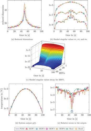
Figure 1 shows the dimensions of the reduced-order models corresponding to solutions of the DLEs based on the different DLE solvers (a), the Hankel singular values ${\sigma }_1$, ${\sigma }_3$ and ${\sigma }_6$ for all integrators (b) and the decay of the Hankel singular values on the entire time horizon (c), respectively. The system outputs of the full and the reduced-order models as well as the related relative errors are depicted in Figures 1(d,e). From these figures one observes that all considered time integrators show basically the same results. In addition, the behaviour of the Hankel singular values appears to be identical for all integration methods, see Figure 1(b). This is, of course, expected, as long as the time integrators find the ‘correct’ solution to the DLEs (3) and (4).

Figure 1. Heated beam: (a) dimensions of the reduced state at different times, (b) the Hankel singular values ${\sigma }_1$, ${\sigma }_3$ and ${\sigma }_6$ for the BDF methods of order $1$, $2$, $3$ and, $6$ and the Rosenbrock schemes of order $1$ and $2$, (c) Hankel singular values for the BDF method of order 1, (d) the outputs of the full and the reduced-order models and (e) relative errors in the output.

4.2. Example 2

The second example describes a heat transfer model originating from an optimal cooling problem for the steel profile given in ref. [24]. In order to obtain an LTV model, we have introduced an artificial time variability to the heat conduction coefficient entering the system matrix $A$. As a result, we have the system (1) with constant matrices $E,B,C$ and a time-varying system matrix $A(t)=\alpha (t)A$ with $\alpha (t)=\frac{3}{4}sin\left(\frac{2\pi t}{T}\right)+1$. This system has dimension $n=1\hspace{0.17em}357$, $m=7$ inputs and $p=6$ outputs. The solution is computed on the time interval $[0,720]s$ with a time integration step size of $\tau =3.6s$ and an input $u(t)={50}^{\circ }C$ describing the heating of the steel profile. The Hankel singular values were truncated at a tolerance of 1 × 10^–5. The computation times for the solution of the DLEs and the square root method are given in Table 3. The behaviour of the timings is similar to the previous example.

Table 3. Steel profile: the computation time for solving the DLE and the square root method.

Method		BDF1	BDF2	BDF3	BDF6	Ros1	Ros2
Time [s]	DLE	6 993.58	7 634.43	8 008.14	10 136.86	6 994.55	35 374.41
	SRM	6.15	8.83	7.46	12.56	6.37	13.71

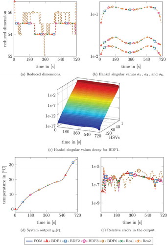
As for the first example, Figure 2 shows the reduced orders obtained by the different DLE solvers (a), the Hankel singular values ${\sigma }_1$, ${\sigma }_3$ and ${\sigma }_6$ (b), and the Hankel singular values decay (c). Further, Figures 2(d,e) depict the output trajectories of the full and the reduced-order models as well as the associated relative errors, respectively. In terms of their quality, these results are similar to those in the example above. Still, we observe that the BDF method of order $6$ yields a wildly oscillating reduced-order and also a slightly worse relative error in the time interval $t\in [360,720]$. An explanation might be given by the fact that the stability region of the BDF methods decreases for an increasing order $s$. In particular methods of order $s>6$ are unstable as it is well known from the theory of BDF methods for ODEs. Furthermore, the stability region depends on the time step size. That is, for a certain step size $\tau$ the results of the higher order methods might be worse. For a detailed discussion on stability of multistep methods for ODEs, see, for example, refs. [21] and [25].

Figure 2. Steel profile: (a) dimensions of the reduced state at different times, (b) the Hankel singular values ${\sigma }_1$, ${\sigma }_3$ and ${\sigma }_6$ for the BDF methods of order $1$, $2$, $3$ and $6$ and the Rosenbrock schemes of order $1$ and $2$, (c) Hankel singular values for the BDF method of order 1, (d) the outputs of the full and the reduced-order models and (e) relative errors in the output.

4.3. Example 3

In the third example, we consider the 1D Burgers equation,

(20) $\begin{array}{cccc}\dot{x}(t,z)& =\nu \frac{{\partial }^2}{\partial z^2}x(t,z)-x(t,z)\frac{\partial }{\partial z}x(t,z)+u(t,z),& \hspace{0.17em}& (t,z)\in (0,T)\times (0,1),\\ x(t,0)& =0,x(t,1)=0,& & t\in (0,T),\\ x(0,z)& =x_0(z),& & z\in (0,1),\end{array}$(20)

describing a convection–diffusion problem with the diffusion coefficient v. The Burgers equation models turbulences, see [26–28], and can be used as a model for shock waves, supersonic flow about airfoils, traffic flows, acoustic transmission and many more. A spatial discretization using finite differences yields a nonlinear model equation. In order to obtain a linear model, a linearization around a pre-computed reference trajectory $x_{\mathrm{r}\mathrm{e}\mathrm{f}}$ is applied. The resulting LTV model reads:

(21) $\begin{array}{rl}& E\dot{x}(t)=A(t)\left(x(t)-x_{ref}(t)\right)+Bu(t)+f(t,x_{\mathrm{r}\mathrm{e}\mathrm{f}}(t))\\ & =A(t)x(t)+Bu(t)+\tilde{f}(t,x_{\mathrm{r}\mathrm{e}\mathrm{f}}(t)),\\ & y=Cx(t)\end{array}$(21)

with $E=I_n$ and a time dependency given solely in $A(t)$. For details on the linearization and discretization, see Hein [29], and the references given therein. We consider a SISO system of dimension $n=2\hspace{0.17em}500$. The matrix $B\in {\mathbb{R}}^n$ is constructed in a way such that the input acts on a grid region of $1\mathrm{\%}$ of the grid nodes around the middle of the spatial domain $(0,1)$. That is, $B_i=1$ for $i=floor\left(\frac{n}{2}\right)\pm floor(0.01n)$ and zero, otherwise. Here, floor denotes the MATLAB® built-in function that rounds the argument to the nearest integer value towards zero. The matrix $C\in {\mathbb{R}}^{1\times n}$ observes the grid point 5 spatial steps to the right of the middle point, i.e. $C_i=1$ for $i=floor\left(\frac{n}{2}\right)+5$ and zero, otherwise.

Note that the inhomogeneity $\tilde{f}(t,x_{\mathrm{r}\mathrm{e}\mathrm{f}})$ in (21) does not affect the model reduction procedure. Following the procedure described in ref. [30] for tracking control based on a common trick to handle inhomogeneities presented in, e.g. [31], system (21) can be reformulated into a homogeneous state-space system (1) while the system matrices do not change.

The model is simulated on the time horizon $[0,3]s$ with time step size $\tau =(2e$-$2)s$. The input is chosen to be $u(t)=2(\mathrm{s}\mathrm{i}\mathrm{n}(2\pi t)+1)$ for $t\in [0,T]$. The truncation tolerance for the Hankel singular values was 1 × 10^–7. Analogously to the previous examples, Table 4 shows the computation times for the solution of the DLEs and the square root method. In contrast to the other examples, here the computation time of the BDF method of order $1$ exceeds those of the BDF2 and BDF3 method. This is due to the number of ADI steps taken for the solution of the ALE.

Table 4. Burgers equation: the computation time for solving the DLE and the square root method.

Method		BDF1	BDF2	BDF3	BDF6	Ros1	Ros2
Time [s]	DLE	4 389.66	3 893.65	3 917.39	4 808.24	4 378.24	17 862.08
	SRM	1.23	1.52	1.34	1.64	1.35	1.51

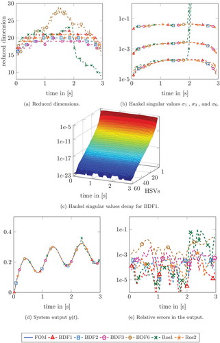
Figure 3 depicts the dimensions of the reduced-order models with respect to the DLE solution methods (a), the Hankel singular values ${\sigma }_1$, ${\sigma }_3$ and ${\sigma }_6$ (b), the Hankel singular values decay over time (c), the output trajectories of the full and the reduced-order models (d), as well as the corresponding relative errors (e). The first-order Rosenbrock method results in an erroneous behaviour of the Hankel singular values. Thus, the reduced-order model is based on a corrupted truncation of the Hankel singular values. Therefore, the results of the Ros1 method in Figure 3 are less accurate compared to the other methods. A number of further computations based on much smaller step sizes $\tau$ led to similar results for all the above methods. That is, for this specific example the Ros1 method requires a smaller step size increasing the computation time in order to achieve the same accuracy compared to the other methods. Further, we observe a decreasing accuracy for an increasing order $s$ of the BDF methods. Here, again we emphasize that the stability region, that among others depends on the step size of the integration procedure, decreases with increasing order.

Figure 3. Burgers equation: (a) dimensions of the reduced state at different times, (b) the Hankel singular values ${\sigma }_1$, ${\sigma }_3$ and ${\sigma }_6$ for the BDF methods of order $1$, $2$, $3$ and $6$ and the Rosenbrock schemes of order $1$ and $2$, (c) Hankel singular values for the BDF method of order 1, (d) the outputs of the full and the reduced-order models and (e) relative errors in the output.

5. Conclusion

In the paper, we have presented the BDF and Rosenbrock time integration methods for the solution of the DLEs arising in the balanced truncation square root method for LTV dynamical systems. Using a low-rank symmetric indefinite factorization for the solution and the indefinite right-hand sides of the ALEs, that have to be solved inside the time integrators, complex data and arithmetic can be avoided. The numerical results show that the proposed integration methods yield satisfactory approximation with respect to the relative errors in the system outputs of the full and the reduced-order models. Further, the given examples show that the performance of the several time integrators strongly depends on the problem under consideration. In addition, regarding the computation time of the reduction bases we have observed that the main effort is to compute the solution to the DLEs. Thus, it might be still a challenge to apply the proposed balanced truncation procedure to LTV systems with a very large system dimension. In particular, the Rosenbrock methods of higher order seem to be very time consuming as one can conjecture from the timings for the two-stage Rosenbrock method.

Another interesting issue that needs to be discussed in the future is the initial and final condition of the reachability and observability Gramians, respectively. These conditions force the reduced state $\hat{x}(t)$ to be zero at the temporal boundaries, i.e. $\hat{x}(0)=\hat{x}(T)=0$, even if the full-order state fulfils $x(0)\ne 0$ and $x(T)\ne 0$. For practical computations, it seems to be necessary to embed the time horizon $[0,T]$ of interest in a sufficiently large interval $[0-\delta ,T+\delta ]$ with $\delta >0$. Furthermore, the time dependent projection matrices do not allow an offline pre-computation of a global reduced-order model. That is, the full order system matrices need to be projected onto the low dimensional subspaces at every time step. Therefore, one should think of a sophisticated strategy to find a global set of projectors based on the time-varying projection bases.

Acknowledgements

This work was supported by the DFG project. The authors would like to thank Maximilian Huber for providing the heated beam example.

Disclosure statement

No potential conflict of interest was reported by the authors.

Additional information

Funding

The first two authors were funded by the DFG project ‘Collaborative Research Center/Transregio 96 Thermo-Energetic Design of Machine Tools’. The third author was supported by the DFG project ‘Model reduction for elastic multibody systems with moving interactions’.

References

- P. Benner, P. Kürschner, and J. Saak, An improved numerical method for balanced truncation for symmetric second order systems, Math. Comput. Model. Dyn. Syst. 19 (2013), pp. 593–615.
- T. Reis and T. Stykel, Balanced truncation model reduction of second-order systems, Math, Comput. Model. Dyn. Syst. 14 (2008), pp. 391–406.
- H. Sandberg and A. Rantzer, Balanced truncation of linear time-varying systems, IEEE Trans. Automat. Control. 49 (2004), pp. 217–229.
- S. Shokoohi, L. Silverman, and P. Van Dooren, Linear time-variable systems: balancing and model reduction, IEEE Trans. Automat. Control. 28 (1983), pp. 810–822.
- E.I. Verriest and T. Kailath, On generalized balanced realizations, IEEE Trans. Automat. Control. 28 (1983), pp. 833–844.
- T. Kailath, Linear Systems, Prentice-Hall, Englewood Cliffs, NJ, 1980.
- A.J. Laub, M.T. Heath, C.C. Paige, and R.C. Ward, Computation of system balancing transformations and other applications of simultaneous diagonalization algorithms, IEEE Trans. Automat. Control. 32 (1987), pp. 115–122.
- M.S. Tombs and I. Postlethwaite, Truncated balanced realization of a stable nonminimal state-space system, Internat. J. Control. 46 (1987), pp. 1319–1330.
- P. Benner and H. Mena, Rosenbrock methods for solving Riccati differential equations, IEEE Trans. Automat. Control. 58 (2013), pp. 2950–2957.
- C. Choi and A.J. Laub, Efficient matrix-valued algorithms for solving stiff Riccati differential equations, IEEE Trans. Automat. Control. 35 (1990), pp. 770–776.
- L. Dieci, Numerical integration of the differential Riccati equation and some related issues, SIAM J. Numer. Anal. 29 (1992), pp. 781–815.
- H. Mena, Numerical solution of differential Riccati equations arising in optimal control problems for parabolic partial differential equations, Ph.D. thesis, Escuela Politecnica Nacional, 2007.
- P. Benner, P. Kürschner, and J. Saak, Efficient handling of complex shift parameters in the low-rank Cholesky factor ADI method, Numer. Algorithms. 62 (2013), pp. 225–251.
- P. Benner, P. Kürschner, and J. Saak, A reformulated low-rank ADI iteration with explicit residual factors, Proc. Appl. Math. Mech. 13 (2013), pp. 585–586.
- J.-R. Li and J. White, Low rank solution of lyapunov equations, SIAM J. Matrix Anal. Appl. 24 (2002), pp. 260–280.
- T. Penzl, Eigenvalue decay bounds for solutions of Lyapunov equations: the symmetric case, Systems Control Lett. 40 (2000), pp. 139–144.
- P. Benner, R.C. Li, and N. Truhar, On the ADI Method for Sylvester equations, J. Comput. Appl. Math. 233 (2009), pp. 1035–1045.
- N. Lang, H. Mena, and J. Saak, On the benefits of the factorization for large-scale differential matrix equation solvers, Linear Algebra Appl. 480 (2015), pp. 44–71.
- M. Bollhöfer and A.K. Eppler, Low-Rank Cholesky Factor Krylov subspace methods for generalized projected Lyapunov equations, in System Reduction for Nanoscale IC Design, P. Benner, ed., Mathematics in Industry, Springer International Publishing, Berlin, Heidelberg, 2016.
- K. Dekker and J.G. Verwer, Stability of Runge-Kutta Methods for Stiff Nonlinear Differential Equations, Elsevier, Amsterdam, 1984.
- E. Hairer and G. Wanner, Solving Ordinary Differential Equations II – Stiff and Differential-Algebraic Problems, Springer Series in Computational Mathematics, Vol. 14, Springer-Verlag, Berlin, Heidelberg, 2002.
- V. Druskin and V. Simoncini, Adaptive rational Krylov subspaces for large-scale dynamical systems, Systems Control Lett. 60 (2011), pp. 546–560.
- J.G. Verwer, E.J. Spee, J.G. Blom, and W. Hundsdorfer, A second Order Rosenbrock method applied to Photochemical dispersion problems, SIAM J. Sci. Comput. 20 (1999), pp. 1456–1480.
- P. Benner and J. Saak, Linear-quadratic regulator design for optimal cooling of steel profiles, Technical Report SFB393/05-05, Sonderforschungsbereich 393 Parallele Numerische Simulation für Physik und Kontinuumsmechanik, TU Chemnitz, D-09107 Chemnitz, 2005 Available from http://www.tu-chemnitz.de/sfb393/sfb05pr.html.
- E. Hairer, S.P. Nørsett, and G. Wanner, Solving Ordinary Differential Equations I – Nonstiff Problems, second, Springer Series in Computational Mathematics, 2nd ed., Vol. 8, Springer-Verlag, Berlin Heidelberg, 1993.
- J.M. Burgers, Application of a model system to illustrate some points of the statistical theory of free turbulence, Proc. Roy. Netherl. Acad. Sci. (Am- sterdam). 43 (1940), pp. 2–12.
- J.M. Burgers, A Mathematical model illustrating the theory of turbulence, Adv. Appl. Mech. 1 (1948), pp. 171–199.
- J.M. Burgers, Statistical problems connected with asymptotic solutions of the one-dimensional nonlinear diffusion equation, in Statistical Models and Turbulence, M. Rosenblatt and C. Van Atta, eds., Lecture Notes in Physics, Vol. 12, Springer, Berlin Heidelberg, 1972, pp. 41–60.
- S. Hein, MPC-LQG-based optimal control of parabolic PDEs, Ph.D. thesis, TU Chemnitz, 2009.
- P. Benner, S. Görner, and J. Saak, Numerical solution of optimal control problems for parabolic systems, in Parallel Algorithms and Cluster Computing. Implementations, Algorithms, and Applications, K.H. Hoffmann and A. Meyer, eds., Lect. Notes Comput. Sci. Eng., Vol. 52, Springer-Verlag, Berlin/Heidelberg, 2006, pp. 151–169.
- S.K. Godunov, Ordinary Differential Equations with Constant Coefficient, Translations of Mathematical Monographs, Vol. 169, AMS, Providence, RI, 1997.