A new framework for H2-optimal model reduction

ABSTRACT

In this contribution, a new framework for ${\mathcal{H}}_2$-optimal reduction is presented, motivated by the local nature of both (tangential) interpolation and ${\mathcal{H}}_2$-optimal approximations. The main advantage is given by a decoupling of the cost of reduction from the cost of optimization, resulting in a significant speedup in ${\mathcal{H}}_2$-optimal reduction. In addition, a middle-sized surrogate model is produced at no additional cost and can be used e.g. for error estimation. Numerical examples illustrate the new framework, showing its effectiveness in producing ${\mathcal{H}}_2$-optimal reduced models at a far lower cost than conventional algorithms. Detailed discussions and optimality proofs are presented for applying this framework to the reduction of multiple-input, multiple-output linear dynamical systems. The paper ends with a brief discussion on how this framework could be extended to other system classes, thus indicating how this truly is a general framework for interpolatory ${\mathcal{H}}_2$ reduction.

KEYWORDS:

• Large scale
• model reduction
• model reduction and model simplification
• ${\mathcal{H}}_2$-optimal reduction

View correction statement:

Erratum

1. Introduction

Recent advances in the development of complex technical systems are partly driven by the advent of software tools that allow their computerized modelling and analysis, drastically reducing the resources required during development. Using information about the system’s geometry, material properties and boundary conditions, a dynamical model can be derived in an almost automated way, allowing for design optimization and verifications using a virtual prototype. Depending on the complexity of the model at hand and the required accuracy during investigation, such models quite easily reach a high complexity. As a consequence, simulations and design optimizations may require excessive computational resources or even become unfeasible. In addition, in some applications the models are required to be evaluated in real-time, e.g. in embedded controllers or digital twins. In this latter case, the computational resources available are particularly limited.

Model reduction is an active field of research aimed at finding numerically efficient algorithms to construct low-order, high-fidelity approximations to the high-order models . Amongst all, the most prominent and numerically tractable methods for linear systems include approximate balanced truncation [1-3] and rational interpolation [4,5]. As these methods generally require only the solution of large sparse systems of equations, they can be applied efficiently even to models of very high order. In a context where the admissible model order is low, e.g. in real-time applications, it is of particular interest to find the best possible approximation for a given order. This problem has been addressed in terms of different error norms (see [6] for Hankel norm, [7] for ${\mathcal{H}}_{\mathrm{\infty }}$ norm), but only for the case of ${\mathcal{H}}_2$-optimal approximations there exist algorithms [8–11] that are both numerically tractable and satisfy optimality conditions. ${\mathcal{H}}_2$-optimal reduction methods are iterative, therefore their numerical efficiency is diminished at slow convergence.

In this contribution, we describe a new reduction framework to increase the numerical efficiency of ${\mathcal{H}}_2$-optimal reduction methods. In this framework, firstly introduced in [12] and further developed in [13] for single-input, single-output (SISO) linear time-invariant (LTI) models, ${\mathcal{H}}_2$-driven optimization is performed in a reduced subspace, lowering the cost with respect to conventional methods. Through the update of this subspace, optimality of the resulting reduced-order model can be established. In this paper we generalize the framework, proving its validity for linear time-invariant system with multiple-inputs and multiple-outputs (MIMO) and indicating possible extensions to further system classes. By applying this framework for ${\mathcal{H}}_2$-optimal reduction, substantial speedup can be achieved. In addition, this framework bears the advantage of producing a Model Function, i.e. a middle-sized surrogate model, at no additional cost. We will give first indications on how to exploit this Model Function in further applications and outline current research endeavours towards this direction.

The remainder of the paper is structured as follows: Section 2 briefly revises ${\mathcal{H}}_2$-optimal reduction for MIMO LTI systems, whereas in Section 3 we analyse the computational cost tied to these methods. Section 4 presents the main result of this contribution, i.e. a new framework for ${\mathcal{H}}_2$-optimal reduction. Section 5 will compare conventional ${\mathcal{H}}_2$-optimal reduction to the new framework in numerical examples and show the potential for significant speedup in reduction time. In Section 6, we indicate how to apply this framework to ${\mathcal{H}}_2$-optimal approaches for different system classes, motivating its general nature. Finally, Section 7 will summarize and conclude the discussion.

2. Preliminaries

2.1. Model reduction by tangential interpolation

Linear dynamical systems are often described by state-space models of the form

(1) $\left.\begin{array}{cc}E\dot{x}(t)& =Ax(t)+Bu(t)\\ y(t)& =Cx(t)\end{array}\right\}\mathrm{\Sigma }$(1)

where $E\in {\mathbb{R}}^{N\times N}$ is the regular descriptor matrix, $A\in {\mathbb{R}}^{N\times N}$ is the system matrix and $x\in {\mathbb{R}}^N$, $u\in {\mathbb{R}}^m$, $y\in {\mathbb{R}}^p$ ($p,m\ll N$) represent the state, input and output of the system, respectively. $\mathrm{\Sigma }$ denotes the system (1) by its state-space representation. The input-output behaviour of a linear system (1) can be characterized in the frequency domain by $y(s)=G(s)u(s)$, with the rational transfer function matrix

(2) $G(s):=C{\left(sE-A\right)}^{-1}B.$(2)

The construction of a reduced-order model (ROM) from the full-order model (FOM) (1) can be obtained by means of a Petrov-Galerkin projection

(3) $\left.\begin{array}{cc}\stackrel{E_r}{\overbrace{W^{\mathrm{T}}EV}}{\dot{x}}_r(t)& =\stackrel{A_r}{\overbrace{W^{\mathrm{T}}AV}}{x}_r(t)+\stackrel{B_r}{\overbrace{W^{\mathrm{T}}B}}u(t)\\ y_r(t)& =\underset{C_r}{\underbrace{CV}}{x}_r(t)\end{array}\right\}{\mathrm{\Sigma }}_r$(3)

with projection matrices $V,W\in {\mathbb{C}}^{N\times n}$ and reduced state vector $x_r\in {\mathbb{R}}^n$ $(n\ll N)$. We will use the shorthand notation ${\mathrm{\Sigma }}_r=W^{\mathrm{T}}\mathrm{\Sigma }V$ to specify the projection matrices used.

The primary goal of model reduction in the following will be the approximation of the output $y(t)\approx y_r(t)$ for all admissible inputs $u(t)$. This is equivalent to approximating the transfer function $G(s)\approx G_r(s)$. To achieve this goal, the appropriate design of projection matrices V,W becomes the primary task of model reduction. In this contribution, we will choose projection matrices that achieve bitangential Hermite interpolation according to following result.

Theorem 2.1 (Bitangential Hermite Interpolation [5,14]) Consider a full-order model $\mathrm{\Sigma }$ as in (1) with transfer function $G(s)$ and let scalar frequencies ${\sigma }_i\in \mathbb{C}$ and vectors $r_i\in {\mathbb{C}}^m$, $l_j\in {\mathbb{C}}^p$ be given such that ${\sigma }_{i}E-A$ is nonsingular for $i=1,\dots ,n$. Consider a reduced-order model ${\mathrm{\Sigma }}_r$ as in (3) with transfer function $G_r(s)$, obtained through projection ${\mathrm{\Sigma }}_r=W^{\mathrm{T}}\mathrm{\Sigma }V$. Let $\mathcal{R}(V)$ denote the range of the matrix $V$.

(1) If

(4) $(A-{\sigma }_{i}E{)}^{-1}B{r}_i\in \mathcal{R}(V),i=1,\dots ,n$(4)

then $G({\sigma }_i)r_i=G_r({\sigma }_i)r_i$.

(2) If

(5) $(A-{\sigma }_{i}E{)}^{-\mathrm{T}}{C}^{\mathrm{T}}{l}_i\in \mathcal{R}(W),i=1,\dots ,n$(5)

then $l_i^{\mathrm{T}}G({\sigma }_i)=l_i^{\mathrm{T}}{G}_r({\sigma }_i)$.

(3) If both (4) and (5) hold, then

(6) $l_i^{\mathrm{T}}{G}^{\prime }({\sigma }_i)r_i=l_i^{\mathrm{T}}{G}_{r^{\prime }}({\sigma }_i)r_i,i=1,\dots ,n,$(6)

where $G^{\prime }(s)$ denotes the first derivative with respect to $s$.

In addition, note that it is possible to tangentially interpolate higher order derivatives $G^{(k)}(s)$ at frequencies ${\sigma }_i\in \mathbb{C}$ by spanning appropriate Krylov subspaces [4,14]. In general, Krylov subspaces are defined through a matrix $M\in {\mathbb{C}}^{N\times N}$, a vector $v\in {\mathbb{C}}^N$ and a scalar $n\in \mathbb{N}$ as follows:

(7) ${\mathcal{K}}_n(M,v)=\mathcal{R}\left(\left[\begin{array}{ccccc}v& Mv& M^{2}v& \dots & M^{n-1}v\end{array}\right]\right).$(7)

Theorem 2.2 (Tangential Moment Matching [4,14]) Consider a full-order model $\mathrm{\Sigma }$ as in (1) with transfer function $G(s)$ and let a scalar frequency $\sigma \in \mathbb{C}$ and nonzero vectors $r\in {\mathbb{C}}^m$, $l\in {\mathbb{C}}^p$ be given, such that $\sigma E-A$ is nonsingular. Consider a reduced-order model ${\mathrm{\Sigma }}_r$ as in (3) with transfer function $G_r(s)$, obtained through the projection ${\mathrm{\Sigma }}_r=W^{\mathrm{T}}\mathrm{\Sigma }V$.

(1) If

(8) ${\mathcal{K}}_n\left({(A-\sigma E)}^{-1}E,(A-\sigma E{)}^{-1}Br\right)\subseteq \mathcal{R}(V),$(8)

then $G^{(i)}(\sigma )r=G_r^{(i)}(\sigma )r$ for $i=0,\dots ,n-1$.

(2) If

(9) ${\mathcal{K}}_n\left({(A-\sigma E)}^{-\mathrm{T}}{E}^{\mathrm{T}},(A-\sigma E{)}^{-\mathrm{T}}{C}^{\mathrm{T}}l\right)\subseteq \mathcal{R}(W),$(9)

then $l^{\mathrm{T}}{G}^{(i)}(\sigma )=l^{\mathrm{T}}{G}_r^{(i)}(\sigma )$ for $i=0,\dots ,n-1$.

(3) If both (8) and (9) hold, then

(10) $l^{\mathrm{T}}{G}^{(i)}(\sigma )r=l^{\mathrm{T}}{G}_r^{(i)}(\sigma )r,i=n,\dots ,2n-1.$(10)

Any bases V and W satisfying (4) and (5) are valid; for theoretical considerations, primitive bases are of particular interest, as defined in the following.

Definition 2.3 (Primitive bases) Consider a full-order model $\mathrm{\Sigma }$ as in (1). Let interpolation frequencies ${\sigma }_i\in \mathbb{C}$ and tangential directions $r_i\in {\mathbb{C}}^m$ and $l_i\in {\mathbb{C}}^p$ be given such that $A-{\sigma }_{i}E$ is invertible for all $i=1,\dots ,n$. Then the primitive projection bases $V^P$, $W^P$ are defined as

(11a) $V^P=\left[{(A-{\sigma }_{1}E)}^{-1}B{r}_1,\dots ,{(A-{\sigma }_{n}E)}^{-1}B{r}_n\right]$(11a)

(11b) $W^P=\left[{(A-{\sigma }_{1}E)}^{-\mathrm{T}}{C}^{\mathrm{T}}{l}_1,\dots ,{(A-{\sigma }_{n}E)}^{-\mathrm{T}}{C}^{\mathrm{T}}{l}_n\right]$(11b)

From a numerical standpoint, $V$ and $W$ are preferably (bi-)orthogonal, real bases, improving the conditioning and resulting in a ${\mathrm{\Sigma }}_R$ with real matrices. Finally, note that the primitive bases (11) can be defined as solutions of particular generalized dense-sparse Sylvester equations.

Lemma 2.4 ([14,15]) Consider a full-order model $\mathrm{\Sigma }$ as in (1). Let interpolation frequencies ${\sigma }_i\in \mathbb{C}$ and tangential directions $r_i\in {\mathbb{C}}^m$ be given such that $A-{\sigma }_{i}E$ is invertible for all $i=1,\dots ,n$. Define matrices $S^P=\mathrm{d}\mathrm{i}\mathrm{a}\mathrm{g}\left({\sigma }_1,\dots ,{\sigma }_n\right)$, $R^P=\left[r_1,\dots ,r_n\right]$. Then the primitive basis $V^P$ satisfying (11a) solves the generalized sparse-dense Sylvester equation

(12) $A{V}^P-E{V}^P{S}^P-B{R}^P=0.$(12)

This relationship is particularly useful for theoretical considerations and will be exploited in Section 4 in the proofs. A dual result for $W^P$ holds as well.

Lemma 2.5 Consider a full-order model $\mathrm{\Sigma }$ as in (1). Let interpolation frequencies ${\sigma }_i\in \mathbb{C}$ and tangential directions $l_i\in {\mathbb{C}}^p$ be given such that $A-{\sigma }_{i}E$ is invertible for all $i=1,\dots ,n$. Define matrices $S^P=\mathrm{d}\mathrm{i}\mathrm{a}\mathrm{g}\left({\sigma }_1,\dots ,{\sigma }_n\right)$, $L^P=\left[l_1,\dots ,l_n\right]$. Then the primitive basis $W^P$ satisfying (11b) solves the generalized sparse-dense Sylvester equation

(13) $A^{\mathrm{T}}{W}^P-E^{\mathrm{T}}{W}^P{S}^P-C^{\mathrm{T}}{L}^P=0.$(13)

2.2. ${\mathscr{H}}_2$-optimal reduction

For the design of V and W as of Section 2.1, an appropriate choice for the interpolation frequencies ${\left\{{\sigma }_i\right\}}_{i=1}^n$ and tangential directions ${\left\{r_i\right\}}_{i=1}^n$, ${\left\{l_i\right\}}_{i=1}^n$ needs to be made. This is a non-trivial task, as the inspection of the FOM is a computationally challenging task in the large-scale setting. For this reason, an automatic selection of reduction parameters minimizing the approximation error $\parallel G-G_r{\parallel }_{\hspace{0.17em}}$ for some chosen norm is highly desirable.

In this contribution, we address the problem of finding an optimal ROM of prescribed order $n$ that minimizes the error measured in the ${\mathcal{H}}_2$ norm, i.e.

(14) $G_r=arg\underset{\mathrm{d}\mathrm{e}\mathrm{g}{\hat{G}}_r=n}{min}\parallel G-{\hat{G}}_r{\parallel }_{{\mathcal{H}}_2},$(14)

where the ${\mathcal{H}}_2$ norm is defined as [16]

(15) $\parallel G{\parallel }_{{\mathcal{H}}_2}:={\left(\frac{1}{2\pi }\underset{-\mathrm{\infty }}{\overset{\mathrm{\infty }}{\int }}\mathrm{t}\mathrm{r}\left(G^H(-j\omega )G(j\omega )\right)\mathrm{d}\omega \right)}^{1/2}.$(15)

Note that there exists a direct relation between the approximation error in the frequency domain in terms of the ${\mathcal{H}}_2$ norm and a bound for the $L_{\mathrm{\infty }}$ norm of the output error in the time domain, according to [17]

(16) $\parallel y-y_r{\parallel }_{L_{\mathrm{\infty }}}\le \parallel G-G_r{\parallel }_{{\mathcal{H}}_2}\parallel u{\parallel }_{L_2}.$(16)

The optimization problem (14) is non-convex, therefore in general only local optima can be found. Necessary conditions for local ${\mathcal{H}}_2$-optimality in terms of bitangential Hermite interpolation are available.

Theorem 2.6 ([8,9,18]) Consider a full-order model (1) with transfer function $G(s)$. Consider a reduced-order model with transfer function $G_r(s)=\sum _{i=1}^n\frac{{\hat{c}}_i{\hat{b}}_i}{s-{\lambda }_{r,i}}$ with reduced poles ${\lambda }_{r,i}\in \mathbb{C}$ and input resp. output residue directions ${\hat{b}}_i^{\mathrm{T}}\in {\mathbb{C}}^m$, ${\hat{c}}_i\in {\mathbb{C}}^p$.

If $G_r(s)$ satisfies (14) locally, then

(17a) $G(-{\bar{\lambda }}_{r,i}){\hat{b}}_i^{\mathrm{T}}=G_r(-{\bar{\lambda }}_{r,i}){\hat{b}}_i^{\mathrm{T}}$(17a)

(17b) ${\hat{c}}_i^{\mathrm{T}}G(-{\bar{\lambda }}_{r,i})={\hat{c}}_i^{\mathrm{T}}{G}_r(-{\bar{\lambda }}_{r,i})$(17b)

(17c) ${\hat{c}}_i^{\mathrm{T}}{G}^{\prime }(-{\bar{\lambda }}_{r,i}){\hat{b}}_i^{\mathrm{T}}={\hat{c}}_i^{\mathrm{T}}{G}_r^{\prime }(-{\bar{\lambda }}_{r,i}){\hat{b}}_i^{\mathrm{T}}$(17c)

for $i=1,\dots ,n$.

Theorem 2.1 indicates how to construct bitangential Hermite interpolants for given interpolation data. However, in general, the eigenvalues and residue direction of the reduced-order model are not known a priori. For this reason, an iterative scheme known as Iterative Rational Krylov Algorithm (IRKA) has been developed [8,9] to iteratively adapt the interpolation data until the conditions (17) are satisfied. A sketch is given in Algorithm 1.

Algorithm 1 MIMO ${\mathcal{H}}_2$-Optimal Tangential Interpolation (IRKA)

Input: FOM $\mathrm{\Sigma }$; Initial interpolation data $S^P$, $R^P$, $L^P$

Output:locally ${\mathcal{H}}_2$-optimal reduced model ${\mathrm{\Sigma }}_r$

1:while not converged do

2: $V^P\leftarrow A{V}^P-E{V}^P{S}^P-B{R}^P=0$          //projection matrix (11a)

3: $W^P\leftarrow A^{\mathrm{T}}{W}^P-E^{\mathrm{T}}{W}^P{S}^P-C^{\mathrm{T}}{L}^P=0$        //projection matrix (11b)

4: $V\leftarrow \mathrm{q}\mathrm{r}(V^P)$; $W\leftarrow \mathrm{q}\mathrm{r}(W^P)$          //compute orthonormal bases

5: ${\mathrm{\Sigma }}_r\leftarrow W^{\mathrm{T}}\mathrm{\Sigma }V$            //compute reduced model by projection

6: [$X,D,Y$] = eig(${\mathrm{\Sigma }}_r$)                 //eigendecomposition

7: $S^P\leftarrow -D;R^P\leftarrow B_r^{\mathrm{T}}Y;L^P\leftarrow C_{r}X$         //update interpolation data

8: end while

Note that the primitive bases in lines 2 and 3 are not computed solving Sylvester equations but rather the sparse linear systems in (11). The equivalent representation using Sylvester equations (cf. Theorem 2.4) is used for brevity.

Finally, note that Algorithm 1 is not the only ${\mathcal{H}}_2$-optimal method for linear systems present in literature, but is certainly best known due to its simplicity and effectiveness. Other approaches worth mentioning include the trust-region algorithms in [10] and [11]. In addition [19], derives a residue correction algorithm to optimize the tangential directions for fixed poles, speeding up convergence for models with many inputs and outputs. Even though for brevity we will not treat all these algorithms individually, the proofs of Section 4 will make evident that the new framework presented in this paper applies to these algorithms as well, as all methods are targeted at satisfying the optimality conditions (17).

3. The cost of ${\mathcal{H}}_2$-optimal reduction

The computational cost of model reduction by IRKA (cf. Algorithm 1) is dominated by the large-scale linear systems of equations (LSE) involved in computing $V^P$, $W^P$ according to

(18a) $\stackrel{=:A_{{\sigma }_i}}{\overbrace{\left(A-{\sigma }_{i}E\right)}}{V}_i^P=B{r}_i,i=1,\dots ,n,$(18a)

(18b) $A_{{\sigma }_i}^{\mathrm{T}}{W}_i^P=C^{\mathrm{T}}{l}_{i}i=1,\dots ,n.$(18b)

In fact, the orthogonalization, the matrix-matrix multiplications involved in the projection ${\mathrm{\Sigma }}_r=W^{\mathrm{T}}\mathrm{\Sigma }V$, and the low-dimensional eigenvalue decomposition are in general of subordinated importance¹. As the matrix $A_{{\sigma }_i}$ of large-scale systems is generally sparse [20], the actual cost involved in solving one LSE depends on a series of factors (including sparsity pattern, number of nonzero elements, conditioning …) as well as the effective exploitation of available hardware resources. It is therefore not possible (or even meaningful) to perform asymptotic operation counts as in the dense case. Nonetheless, to demonstrate that the reduction cost is indeed dominated by the solution of the sparse LSE in (18), Figure 1 compares the average execution times for the different computation steps of Algorithm 1 using MATLAB® R2016b on an Intel® Core™ i7-2640 CPU @ 2.80 GHz computer with 8GB RAM.

Figure 1. Cumulated execution times involved in each step of algorithm 1 for different benchmark models ($n=10$).

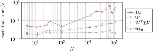
The comparison includes the sparse lu decomposition of the matrix $A-E$, the economy-sized qr decomposition of the projection matrix $V^P$, the matrix products involved in $W^{\mathrm{T}}\mathrm{\Sigma }V$ as well as the small dimensional generalized eig decompositions. The reduced order is set to n = 10 for all cases, while the original model order is given on the x-axis. The times given are averaged amongst several executions and cumulated for each IRKA step: At each iteration of IRKA, n lu decompositions, two qr decompositions, one projection $W^{\mathrm{T}}\mathrm{\Sigma }V$ and one eig decomposition are performed. The models used are taken from the benchmark collections [21,22].

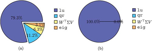
As it can be seen, the execution time for the sparse lu decompositions grows more and more dominant as the problem size increases. This becomes even more evident in Figure 2, where the execution times are given as percentage of the total time for one IRKA iteration. The two models shown represent the extreme cases of Figure 1, i.e. where the execution time for the lu decompositions has the smallest and largest share.

Figure 2. Cumulated execution times as total share of each step of Algorithm 1.

IRKA (and alternative ${\mathcal{H}}_2$ reduction methods) require the repeated reduction of an Nth-order model until, after $k_{{\mathcal{H}}_2}$ steps, a set of ${\mathcal{H}}_2$-optimal parameters ${\left\{{\sigma }_{\ast ,i}\right\}}_{i=1}^n$, ${\left\{r_{\ast ,i}\right\}}_{i=1}^n$, and ${\left\{l_{\ast ,i}\right\}}_{i=1}^n$ is found. Following the results of Figures 1 and 2, its cost can be approximated by

(19) ${\mathcal{C}}_N\left(\mathrm{I}\mathrm{R}\mathrm{K}\mathrm{A}\right)\approx \underset{optimization}{\underbrace{k_{{\mathcal{H}}_2}}}\cdot \underset{reduction}{\underbrace{2n{\mathcal{C}}_N\left(\mathrm{L}\mathrm{S}\mathrm{E}\right)}},$(19)

where the cost of a $N$-dimensional LSE ${\mathcal{C}}_N\left(\mathrm{L}\mathrm{S}\mathrm{E}\right)$ depends on, amongst others, the model at hand, as well as the chosen LSE solver². While the second factor in (19) represents the cost of a single reduction, the factor $k_{{\mathcal{H}}_2}$ represents the cost introduced by the optimization. From this representation, it becomes evident that the cost of optimization is tied to – in fact weighted with – the cost of a full reduction. The efficiency of ${\mathcal{H}}_2$-optimal reduction methods can hence be significantly deteriorated by bad convergence, which can be a result of a bad initialization or the selection of an unsuitable reduced order. A very similar discussion applies to trust-region-based ${\mathcal{H}}_2$-optimal reduction methods [10,11], where the evaluation of gradient and Hessian in each step also involves a full reduction.

Clearly, a more desirable setting would be to obtain ${\mathcal{H}}_2$-optimal reduction parameters at a far lower cost than the cost of reduction, having to reduce the full-order model only once. In the following, we introduce a new framework that effectively decouples the cost of reduction from the cost of finding ${\mathcal{H}}_2$-optimal reduction parameters without compromising optimality.

4. A new framework for ${\mathcal{H}}_2$-optimal reduction

The framework discussed in this section was first introduced in [12, p. 83] for SISO models, under the name of model function, a heuristic to reduce the cost of ${\mathcal{H}}_2$-optimal reduction within the SPARK algorithm. This heuristic was later applied to IRKA and proved in [13] to yield ${\mathcal{H}}_2$-optimal reduced-order models under certain update conditions. In this contribution, we give a more extensive discussion of the framework, extending its validity to MIMO models. In Section 6, we will indicate how to apply this framework also to further system classes for which ${\mathcal{H}}_2$ approximation algorithms are available. The main motivation for the new framework arises from simple considerations on the locality of ${\mathcal{H}}_2$-optimal model reduction by tangential interpolation. In fact,

1. tangential interpolation only guarantees to yield a good approximation locally around the frequencies ${\left\{{\sigma }_i\right\}}_{i=1}^n$, tangentially along directions ${\left\{r_i\right\}}_{i=1}^n$ and ${\left\{l_i\right\}}_{i=1}^n$,

2. as $\parallel G-G_r{\parallel }_{{\mathcal{H}}_2}$ is a non-convex function, in general only local optima can be achieved.

This can be exploited during reduction as follows: Suppose a full-order model $\mathrm{\Sigma }$ and initial tangential interpolation data ${\left\{{\sigma }_i^0\right\}}_{i=1}^n$,${\left\{r_i^0\right\}}_{i=1}^n$, and ${\left\{l_i^0\right\}}_{i=1}^n$ are given. Conventional ${\mathcal{H}}_2$ reduction approaches would initialize e.g. IRKA and run for $k_{{\mathcal{H}}_2}$ steps until convergence. In contrast, as our goal is to find a local optimum close to the initialization, then optimization with respect to a surrogate model – a good local approximation with respect to the initial interpolation data – may suffice. For this reason, the new framework starts by building an intermediate model ${\mathrm{\Sigma }}_{\mu }$ – in the following denoted as Model Function, in accordance to its first introduction in [12] – of order $n_{\mu }$, with $N\gg n_{\mu }>n$.

Definition 4.1 Consider a full-order model $\mathrm{\Sigma }$ as in (1). Let interpolation data ${\sigma }_{\mu ,i}\in \mathbb{C}$, $r_{\mu ,i}\in {\mathbb{C}}^m$, $l_{\mu ,i}\in {\mathbb{C}}^p$, $i=1,\dots ,n_{\mu }$, be given and define the matrices $S_{\mu }=\mathrm{d}\mathrm{i}\mathrm{a}\mathrm{g}\left({\sigma }_{\mu ,1},\dots ,{\sigma }_{\mu ,n_{\mu }}\right)$, $R_{\mu }=\left[\begin{array}{ccc}{r}_{\mu ,1}& \dots & r_{\mu ,n_{\mu }}\end{array}\right]$, $L_{\mu }=\left[\begin{array}{ccc}{l}_{\mu ,1}& \dots & l_{\mu ,n_{\mu }}\end{array}\right]$. Then the Model Function ${\mathrm{\Sigma }}_{\mu }$ is defined as

(20) ${\mathrm{\Sigma }}_{\mu }:=W_{\mu }\mathrm{\Sigma }{V}_{\mu },$(20)

where $V_{\mu },W_{\mu }$ solve the Sylvester equations

(21a) $A{V}_{\mu }-E{V}_{\mu }{S}_{\mu }-B{R}_{\mu }=0,$(21a)

(21b) $A^{\mathrm{T}}{W}_{\mu }-E^{\mathrm{T}}{W}_{\mu }{S}_{\mu }-C^{\mathrm{T}}{L}_{\mu }=0.$(21b)

From Theorem 4.1 and the results of Theorem 2.4, Theorem 2.5, and Theorem 2.1 it follows that ${\mathrm{\Sigma }}_{\mu }$ is a bitangential Hermite interpolant of $\mathrm{\Sigma }$ with interpolation frequencies and tangential directions specified in $S_{\mu }$, $R_{\mu }$ and $L_{\mu }$.

4.1. The Model Function framework

Step 1: Initialization of ${\mathrm{\Sigma }}_{\mu }$The goal of the Model Function ${\mathrm{\Sigma }}_{\mu }$ is to be a good approximation of $\mathrm{\Sigma }$, locally with respect to the initial interpolation data ${\left\{{\sigma }_i^0\right\}}_{i=1}^n$, ${\left\{r_i^0\right\}}_{i=1}^n$, and ${\left\{l_i^0\right\}}_{i=1}^n$, for it to be used as a surrogate of $\mathrm{\Sigma }$ during the ${\mathcal{H}}_2$ optimization. For obvious reasons, it must hold $n_{\mu }>n$, making it not possible to choose $S_{\mu }=S^0:=\mathrm{d}\mathrm{i}\mathrm{a}\mathrm{g}\left({\sigma }_1^0,\dots ,{\sigma }_n^0\right)$, $R_{\mu }=R^0:=\left[\begin{array}{ccc}{r}_1^0& \dots & r_n^0\end{array}\right]$, and $L_{\mu }=L^0:=\left[\begin{array}{ccc}{l}_{,1}^0& \dots & l_n^0\end{array}\right]$. In the following, we introduce two possible alternatives:

I.1 Include the initial interpolation data $S^0,R^0,L^0$ with additional interpolation of $G(s)$ and its first $n_{\mu }-n-1$ derivatives at the frequency $\sigma =0$ for a sum of all input and output channels. This can be achieved through

(22) $\begin{array}{c}\begin{array}{cc}{S}_{\mu }=\left[\begin{array}{cc}{S}^0& 0\\ 0& J_0\end{array}\right],R_{\mu }& =\left[\begin{array}{ccccc}{R}^0& e_1& 0& \dots & 0\end{array}\right],\\ L_{\mu }& =\left[\begin{array}{ccccc}{L}^0& e_1& 0& \dots & 0\end{array}\right],\end{array}\\ \hspace{0.17em}\end{array}$(22)

where $J_0$ is a Jordan block of size $n_{\mu }-n$ with eigenvalue $0$ and $e_1:={\left[\begin{array}{cccc}1& 1& \dots & 1\end{array}\right]}^{\mathrm{T}}$ of appropriate dimensions. In this case, the choice of $n_{\mu }$ is free. Due to Theorem 2.2, we expect the approximation quality of ${\mathrm{\Sigma }}_{\mu }$ to improve locally around $\sigma =0$ as $n_{\mu }$ grows.

1.2 Tangentially interpolate higher-order derivatives with respect to the data $S^0,R^0,L^0$. This can be achieved through

(23) $S_{\mu }=\left[\begin{array}{cc}{S}^0& J_0\\ 0& S^0\end{array}\right],R_{\mu }=\left[\begin{array}{cc}{R}^0& 0\end{array}\right],L_{\mu }=\left[\begin{array}{cc}{L}^0& 0\end{array}\right],$(23)

(cf. Theorem 2.2). In this case $n_{\mu }=2n$ and we expect the approximation quality of ${\mathrm{\Sigma }}_{\mu }$ to increase locally around the frequencies ${\left\{{\sigma }_i^0\right\}}_{i=1}^n$ with respect to the tangential directions ${\left\{r_i^0\right\}}_{i=1}^n$ and ${\left\{l_i^0\right\}}_{i=1}^n$.

Many more choices for $S_{\mu }$, $R_{\mu }$, and $L_{\mu }$ are conceivable and valid. Nonetheless, the approaches presented above bear the advantage of minimizing the additional cost tied to the initialization of ${\mathrm{\Sigma }}_{\mu }$. In fact, note that for every value ${\sigma }_{\mu ,i}={\sigma }_{\mu ,j}$, the LSEs in (18) share the same left-hand side, allowing e.g. the recycling of LU decompositions or pre-conditioners. That said, one may choose to use the additional degrees of freedom to enforce tangential interpolation with respect to different data. As there is no rigorous rule for this – just like there is no rigorous rule on how to initialize ${\mathcal{H}}_2$-optimal reduction – our philosophy is to minimize the initialization cost and let the optimizer choose new frequencies of interest. Finally, note that the specific choice of initialization may affect both the speed of convergence and resulting approximation quality.

Step 2: $\mathcal{H}$₂ optimization with respect to ${\mathrm{\Sigma }}_{\mu }$ As the Model Function ${\mathrm{\Sigma }}_{\mu }$ is a good approximation of $\mathrm{\Sigma }$ locally with respect to the initial interpolation data, we can run the ${\mathcal{H}}_2$ optimization with respect to ${\mathrm{\Sigma }}_{\mu }$ with initialization $S^0$, $R^0$, $L^0$. The optimal interpolation data found at convergence is denoted by $S_{\ast }=\mathrm{d}\mathrm{i}\mathrm{a}\mathrm{g}\left({\sigma }_{\ast ,1},\dots ,{\sigma }_{\ast ,n}\right)$, $R_{\ast }=\left[\begin{array}{ccc}{r}_{\ast ,1}& \dots & r_{\ast ,n}\end{array}\right]$, and $L_{\ast }=\left[\begin{array}{ccc}{l}_{{\ast }_{,}1}& \dots & l_{\ast ,n}\end{array}\right]$. As typically $n_{\mu }\ll N$, we are expecting the cost of this optimization to be significantly lower than a full optimization over $\mathrm{\Sigma }$. As we assume the validity of the resulting reduced-order model ${\mathrm{\Sigma }}_{\mu ,r}$ to be confined locally to the frequency region defined by $S_{\mu }$, we call the combination of IRKA with this Model Function framework Confined IRKA (CIRKA).

In fact, by approximating $\mathrm{\Sigma }$ through ${\mathrm{\Sigma }}_{\mu }$, we have lost any optimality condition between $\mathrm{\Sigma }$ and ${\mathrm{\Sigma }}_{\mu ,r}$. Whether ${\mathrm{\Sigma }}_{\mu ,r}$ is an acceptable approximation of $\mathrm{\Sigma }$ highly depends on the approximation quality of ${\mathrm{\Sigma }}_{\mu }$ itself. This loss of connection between $\mathrm{\Sigma }$ and ${\mathrm{\Sigma }}_{\mu ,r}$ is a typical drawback of so-called two-step model reduction approaches. Nonetheless, by means of surrogate optimization, a new set of interpolation data $S_{\ast }$, $R_{\ast }$, $L_{\ast }$ has been found in a cost-effective way. At this point, an update of ${\mathrm{\Sigma }}_{\mu }$ with local information about these frequencies is required.

Step 3: Update of ${\mathrm{\Sigma }}_{\mu }$ and fixed-point iteration To restore the relationship between $\mathrm{\Sigma }$ and ${\mathrm{\Sigma }}_{\mu ,r}$, the Model Function ${\mathrm{\Sigma }}_{\mu }^k$ from the current step $k$ can be updated to a new ${\mathrm{\Sigma }}_{\mu }^{k+1}$ by enforcing tangential interpolation with respect to the optimal data $S_{\ast }^k$, $R_{\ast }^k$, $L_{\ast }^k$. This can be achieved by updating the projection matrices

(24a) $V_{\mu }^{k+1}=\left[V_{\mu }^k\hspace{0.17em}{V}_{\mu }^{k,+}\right]\hspace{0.17em},$(24a)

(24b) $W_{\mu }^{k+1}=\left[\hspace{0.17em}{W}_{\mu }^k\hspace{0.17em}{W}_{\mu }^{k,+}\right]\hspace{0.17em},$(24b)

with new directions $V_{\mu }^{k,+}$ and $W_{\mu }^{k,+}$. As for the initialization of ${\mathrm{\Sigma }}_{\mu }^0$, several strategies are possible. In the following, we present only a few most relevant ones:

U.1 Update ${\mathrm{\Sigma }}_{\mu }^k$ with tangential interpolation with respect to all optimal frequencies and tangential directions $S_{\ast }^k$, $R_{\ast }^k$, $L_{\ast }^k$. This implies that $n_{\mu }^k$ increases by n in every step and that higher-order derivatives are tangentially interpolated in case specific combinations of optimal frequencies and tangential directions are repeated. In this approach, we expect the approximation quality of ${\mathrm{\Sigma }}_{\mu }^{k+1}$ to increase around all optimal frequencies ${\left\{{\sigma }_{\ast ,i}\right\}}_{i=1}^n$, with respect to the tangential directions ${\left\{r_{\ast ,i}\right\}}_{i=1}^n$ and ${\left\{l_{\ast ,i}\right\}}_{i=1}^n$.

U.2 Update ${\mathrm{\Sigma }}_{\mu }^k$ only with tangential interpolation with respect to new interpolation data. This implies that the order of the Model Function increases by at most $n$ in every step. In this approach, we expect the approximation quality of ${\mathrm{\Sigma }}_{\mu }^{k+1}$ to increase only around new optimal frequencies ${\sigma }_{\ast ,i}$ with respect to the respective tangential directions $r_{\ast ,i}$ and $l_{\ast ,i}$, for $i=1,\dots ,n_{\mu }^{k,+}$, where $n_{\mu }^{k,+}$ denotes the number of new frequencies.

U.3 Reinitialize ${\mathrm{\Sigma }}_{\mu }^k$ by including ‘only’ tangential interpolation about the new optimal data. In this approach, we expect the approximation quality of ${\mathrm{\Sigma }}_{\mu }^{k+1}$ to increase in the regions around the new optimal frequencies ${\left\{{\sigma }_{\ast ,i}\right\}}_{i=1}^n$, with respect to the tangential directions ${\left\{r_{\ast ,i}\right\}}_{i=1}^n$ and ${\left\{l_{\ast ,i}\right\}}_{i=1}^n$, but potentially decrease around previous interpolation data. However, the order $n_{\mu }^k$ can be kept constant through iterations using this method, reducing the cost of ${\mathcal{H}}_2$ optimization. As $n_{\mu }^k>n$, similar considerations apply as for the Initialization in Step 1.

The updated Model Function ${\mathrm{\Sigma }}_{\mu }^{k+1}$ can be used again to perform a low-dimensional ${\mathcal{H}}_2$ optimization and potentially improve the optimal frequencies and directions $S_{\ast }^{k+1}$,$R_{\ast }^{k+1}$ and $L_{\ast }^{k+1}$, which in general may differ from those of the previous step. This leads to a fixed-point iteration, until, after $k_{\mu }$ steps, an update of ${\mathrm{\Sigma }}_{\mu }^{k_{\mu }-1}$ does not result in new optimal interpolation data.

The overall procedure is summarized in Algorithm 2 for the case where ${\mathcal{H}}_2$ optimization is performed with IRKA. Note however that Line 6 can be replaced by any ${\mathcal{H}}_2$-optimal reduction method, leading to the more general Model Function framework. Also note that Line 5 covers both the initialization and the update of the Model Function. For brevity, details on the implementation are omitted at this point. MATLAB® code for the proposed algorithms is provided with this paper as functions of the sssMOR toolbox [24].

Algorithm 2 Confined IRKA (CIRKA)

Input: FOM $\mathrm{\Sigma }$; Initial interpolation data $S^0$, $R^0$, $L^0$

Output: reduced model ${\mathrm{\Sigma }}_{\mu ,r}$, Model Function ${\mathrm{\Sigma }}_{\mu }^{k_{\mu }}$, error estimation ${\widetilde{ϵ}}_{{\mathcal{H}}_2}$

1: $k\leftarrow 0$; $\left[{\mathrm{\Sigma }}_{\mu }^k,S_{\ast }^{\mathrm{t}\mathrm{o}\mathrm{t}},R_{\ast }^{\mathrm{t}\mathrm{o}\mathrm{t}},L_{\ast }^{\mathrm{t}\mathrm{o}\mathrm{t}}\right]\leftarrow$ empty;            //Initialization

2: $S_{\ast }^k\leftarrow S^0$, $R_{\ast }^k\leftarrow R^0$, $L_{\ast }^k\leftarrow L^0$;

3: while not converged do

4: $k\leftarrow k+1$

5: ${\mathrm{\Sigma }}_{\mu }^k\leftarrow$updateModelFunction$\left(\mathrm{\Sigma },{\mathrm{\Sigma }}_{\mu }^{k-1},S_{\ast }^{\mathrm{t}\mathrm{o}\mathrm{t}},R_{\ast }^{\mathrm{t}\mathrm{o}\mathrm{t}},L_{\ast }^{\mathrm{t}\mathrm{o}\mathrm{t}},S_{\ast }^{k-1},R_{\ast }^{k-1},L_{\ast }^{k-1}\right)$

6: $\left[{\mathrm{\Sigma }}_{\mu ,r},S_{\ast }^k,R_{\ast }^k,L_{\ast }^k\right]\leftarrow$ IRKA $({\mathrm{\Sigma }}_{\mu }^k,S_{\ast }^{k-1},R_{\ast }^{k-1},L_{\ast }^{k-1})$

7: $S_{\ast }^{\mathrm{t}\mathrm{o}\mathrm{t}}\leftarrow$blkdiag$\left(S_{\ast }^{\mathrm{t}\mathrm{o}\mathrm{t}},S_{\ast }^k\right)$; $R_{\ast }^{\mathrm{t}\mathrm{o}\mathrm{t}}\leftarrow \left[R_{\ast }^{\mathrm{t}\mathrm{o}\mathrm{t}},R_{\ast }^k\right]$; $L_{\ast }^{\mathrm{t}\mathrm{o}\mathrm{t}}\leftarrow \left[L_{\ast }^{\mathrm{t}\mathrm{o}\mathrm{t}},L_{\ast }^k\right]$

8: end while

9: $k_{\mu }\leftarrow k$

10: ${\widetilde{ϵ}}_{{\mathcal{H}}_2}\leftarrow$norm$\left(G_{\mu }^{k_{\mu }}-G_{\mu ,r}\right)$

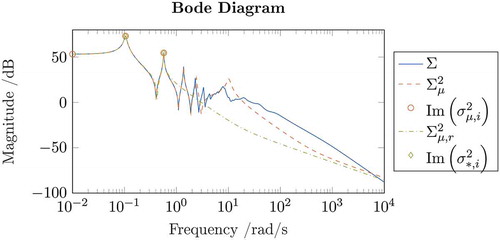
4.2. An illustrative example

To make the explanation of the framework clearer, we include a simple numerical example to accompany the discussion. As a test model we consider the benchmark model beam [21] of order $N=348$ with $m=p=1$. Our aim is to find a model of reduced order $n=4$ satisfying ${\mathcal{H}}_2$-optimality conditions. We assume that no previous information about the relevant frequency region is given, hence the initialization is chosen with interpolation frequencies ${\sigma }_1^0=\dots ={\sigma }_n^0=0$, corresponding to $S^0=J_0$. As the model is SISO, there is no need to specify tangential directions.

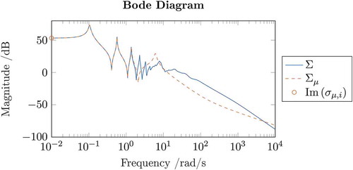
Step 1: Initialization of ${\mathrm{\Sigma }}_{\mu }$ As initial order for the Model Function we select $n_{\mu }=2n=8$. In this particular case, both initializations I.1 and I.2 of ${\mathrm{\Sigma }}_{\mu }$ coincide. Figure 3 shows the Bode plot of $\mathrm{\Sigma }$ and the resulting ${\mathrm{\Sigma }}_{\mu }$³. The orange circles indicate the imaginary part of the frequencies used to initialize the Model Function.

Figure 3. Illustrative Bode plot of $\mathrm{\Sigma }$ and its Model Function ${\mathrm{\Sigma }}_{\mu }$.

Step 2: $\mathcal{H}$₂ optimization with respect to ${\mathrm{\Sigma }}_{\mu }$ Figure 4 shows the reduced-order model ${\mathrm{\Sigma }}_{\mu ,r}$ resulting from the optimization with respect to ${\mathrm{\Sigma }}_{\mu }$.

Figure 4. Comparison of $\mathrm{\Sigma }$, ${\mathrm{\Sigma }}_{\mu }$ and ${\mathrm{\Sigma }}_{\mu ,r}$ after ${\mathcal{H}}_2$ optimization.

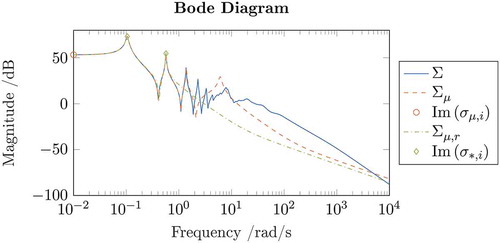
In this example, IRKA converged in $k_{{\mathcal{H}}_2}=4$ steps at optimal frequencies $S_{\ast }=\mathrm{d}\mathrm{i}\mathrm{a}\mathrm{g}\left(\begin{array}{cc}0.005\pm i0.104& 0.006\pm i0.569\end{array}\right)$, whose imaginary parts are depicted in Figure 4 by green diamonds. In this case, by inspection of the Bode plot, we see that ${\mathrm{\Sigma }}_{\mu ,r}$ appears to be an acceptable approximation also of the original model $\mathrm{\Sigma }$ for the given order $n$. This is a result of ${\mathrm{\Sigma }}_{\mu }$ being a valid approximation of $\mathrm{\Sigma }$ also locally around the new frequency region represented by $S_{\ast }$. However, this need not hold true in general. For this reason, an update of the Model Function is performed.

Step 3: Update of ${\mathrm{\Sigma }}_{\mu }$ and fixed-point iteration Using $S_{\ast }^1$, we update ${\mathrm{\Sigma }}_{\mu }^1$ to ${\mathrm{\Sigma }}_{\mu }^2$ by including interpolation of the full-order model $\mathrm{\Sigma }$ with respect to the frequencies in $S_{\ast }^1$. As all optimal frequencies differ from those used for initialization of ${\mathrm{\Sigma }}_{\mu }$, update strategies U.1 and U.2 coincide in this case. Figure 5 shows the updated Model Function ${\mathrm{\Sigma }}_{\mu }^2$ of order $n_{\mu }^2=12$ for the beam example, as well as the reduced-order model ${\mathrm{\Sigma }}_{\mu ,r}^2$ and new optimal frequencies $S_{\ast }^2$ resulting from IRKA on ${\mathrm{\Sigma }}_{\mu }^2$.

Figure 5. Comparison of $\mathrm{\Sigma }$, ${\mathrm{\Sigma }}_{\mu }^2$ and ${\mathrm{\Sigma }}_{\mu ,r}^2$ after repeated ${\mathcal{H}}_2$ optimization.

In this example, IRKA converges (within some tolerance) to the same optimal frequencies $S_{\ast }^2\approx S_{\ast }^1$ and hence the whole framework required $k_{\mu }=2$ iterations until convergence. The fact that an update of the Model Function does not yield a new optimum indicates that the Model Function ${\mathrm{\Sigma }}_{\mu }^1$ was already accurate enough in the region around $S_{\ast }^1$.

Finally, note that while this framework has required 3 full-sized LU decompositions to generate and update the Model Function, a direct application of IRKA to $\mathrm{\Sigma }$ requires $1+(k_{{\mathcal{H}}_2}-1)\cdot n/2=1+3\cdot 2=7$ full-sized LU decompositions, i.e. more than double the amount. A deeper discussion and comparison of the complexities will be given in Section 4.5 and Section 5. It is also worth noting that both CIRKA and IRKA converge to the same local optimum.

4.3. Optimality of the new framework

So far, the new framework has been presented as a heuristic to perform ${\mathcal{H}}_2$ surrogate optimization and – hopefully – reduce the overall reduction cost. The update of ${\mathrm{\Sigma }}_{\mu }^k$ has been introduced to increase the accuracy of the surrogate model in the frequency regions the optimizer seemed to deem as important. However our original intent was to obtain a reduced model ${\mathrm{\Sigma }}_r$ satisfying the ${\mathcal{H}}_2$-optimality conditions (17). The question still remains as to whether this goal has been achieved. In this section, we prove that the update of ${\mathrm{\Sigma }}_{\mu }^k$ is sufficient to satisfy the optimality conditions (17) at convergence.

Theorem 4.2. Consider a full-order model $\mathrm{\Sigma }$ as in (1) with transfer function $G(s)$ . Let $V_{\mu },W_{\mu }\in {\mathbb{C}}^{N\times n_{\mu }}$ satisfy

(25a) $A{V}_{\mu }-E{V}_{\mu }{S}_{\mu }-B{R}_{\mu }=0,$(25a)

(25b) $A^{\mathrm{T}}{W}_{\mu }-E^{\mathrm{T}}{W}_{\mu }{S}_{\mu }-C^{\mathrm{T}}{L}_{\mu }=0,$(25b)

with matrices $S_{\mu }=\mathrm{d}\mathrm{i}\mathrm{a}\mathrm{g}\left({\sigma }_{\mu ,1},\dots ,{\sigma }_{\mu ,n_{\mu }}\right)$, $R_{\mu }=\left[\begin{array}{c}{r}_{\mu ,1},\dots ,r_{\mu ,n_{\mu }}\end{array}\right]$, $L_{\mu }=\left[\begin{array}{c}{l}_{\mu ,1},\dots ,l_{\mu ,n_{\mu }}\end{array}\right]$ and ${\sigma }_{\mu ,j}\in \mathbb{C}$, $r_{\mu ,j}\in {\mathbb{C}}^m$, $l_{\mu ,j}\in {\mathbb{C}}^p$. Consider the Model Function ${\mathrm{\Sigma }}_{\mu }=W_{\mu }^{\mathrm{T}}\mathrm{\Sigma }{V}_{\mu }$ with transfer function $G_{\mu }(s)$ . Let $V_{\mu ,r},W_{\mu ,r}\in {\mathbb{C}}^{n_{\mu }\times n}$ satify

(26a) $A_{\mu }{V}_{\mu ,r}-E_{\mu }{V}_{\mu ,r}{S}_{\ast }-B_{\mu }{R}_{\ast }=0,$(26a)

(26b) $A_{\mu }^{\mathrm{T}}{W}_{\mu ,r}-E_{\mu }^{\mathrm{T}}{W}_{\mu ,r}{S}_{\ast }-C_{\mu }^{\mathrm{T}}{L}_{\ast }=0,$(26b)

with matrices $S_{\ast }=\mathrm{d}\mathrm{i}\mathrm{a}\mathrm{g}\left({\sigma }_{\ast ,1},\dots ,{\sigma }_{\ast ,n}\right)$, $R_{\ast }=\left[\begin{array}{c}{r}_{\ast ,1},\dots ,r_{\ast ,n}\end{array}\right]$, $L_{\ast }=\left[\begin{array}{c}{l}_{\ast ,1},\dots ,l_{\ast ,n}\end{array}\right]$ and ${\sigma }_{\ast ,i}\in \mathbb{C}$, $r_{\ast ,i}\in {\mathbb{C}}^m$, $l_{\ast ,i}\in {\mathbb{C}}^p$. Consider the reduced Model Function ${\mathrm{\Sigma }}_{\mu ,r}={\left(W_{\mu ,r}\right)}^{\mathrm{T}}{\mathrm{\Sigma }}_{\mu }{V}_{\mu ,r}$ with transfer function $G_{\mu ,r}(s)$ . Further, assume that for every $i=1,\dots ,n$, the triplets $\left({\sigma }_{\ast ,i},r_{\ast ,i},l_{\ast ,i}\right)$ satisfy $\left({\sigma }_{\ast ,i},r_{\ast ,i},l_{\ast ,i}\right)=\left(-{\bar{\lambda }}_{r,i},{\hat{b}}_i^{\mathrm{T}},{\hat{c}}_i\right)$ where $G_{\mu ,r}(s)=\sum _{i=1}^n\frac{{\hat{c}}_i{\hat{b}}_i}{s-{\lambda }_{r,i}}$ is the pole/residue representation of the reduced Model Function.

If, for every $i=1,\dots ,n$, there exists a $j=1,\dots ,n_{\mu }$, such that

(27) $\left({\sigma }_{\mu ,j},r_{\mu ,j},l_{\mu ,j}\right)=\left({\sigma }_{\ast ,i},r_{\ast ,i},l_{\ast ,i}\right),$(27)

then ${\mathrm{\Sigma }}_{\mu ,r}$ satisfies the first-order ${\mathcal{H}}_2$ optimality conditions

$G(-{\bar{\lambda }}_{r,i}){\hat{b}}_i^{\mathrm{T}}=G_{\mu ,r}(-{\bar{\lambda }}_{r,i}){\hat{b}}_i^{\mathrm{T}}$

${\hat{c}}_i^{\mathrm{T}}G(-{\bar{\lambda }}_{r,i})={\hat{c}}_i^{\mathrm{T}}{G}_{\mu ,r}(-{\bar{\lambda }}_{r,i})$

${\hat{c}}_i^{\mathrm{T}}{G}^{\prime }(-{\bar{\lambda }}_{r,i}){\hat{b}}_i^{\mathrm{T}}={\hat{c}}_i^{\mathrm{T}}{G}_{\mu ,r}^{\prime }(-{\bar{\lambda }}_{r,i}){\hat{b}}_i^{\mathrm{T}}$

for all $i=1,\dots n$

Proof. By Theorem 2.1 and Theorem 2.4, construction of ${\mathrm{\Sigma }}_{\mu ,r}$ with the projection matrices satisfying (26) results in a reduced model that is a bitangential Hermite interpolant of the Model Function ${\mathrm{\Sigma }}_{\mu }$ with respect to the interpolation data $S_{\ast }$, $R_{\ast }$, and $L_{\ast }$. In combination with the assumption $\left({\sigma }_{\ast ,i},r_{\ast ,i},l_{\ast ,i}\right)=\left(-{\bar{\lambda }}_{r,i},{\hat{b}}_i^{\mathrm{T}},{\hat{c}}_i\right)$, this yields the relationship

(29) $\begin{array}{cc}{G}_{\mu }(-{\bar{\lambda }}_{r,i}){\hat{b}}_i^{\mathrm{T}}& =G_{\mu ,r}(-{\bar{\lambda }}_{r,i}){\hat{b}}_i^{\mathrm{T}},\\ {\hat{c}}_i^{\mathrm{T}}{G}_{\mu }(-{\bar{\lambda }}_{r,i})& ={\hat{c}}_i^{\mathrm{T}}{G}_{\mu ,r}(-{\bar{\lambda }}_{r,i}),\\ {\hat{c}}_i^{\mathrm{T}}{G^{\prime }}_{\mu }(-{\bar{\lambda }}_{r,i}){\hat{b}}_i^{\mathrm{T}}& ={\hat{c}}_i^{\mathrm{T}}{G^{\prime }}_{\mu ,r}(-{\bar{\lambda }}_{r,i}){\hat{b}}_i^{\mathrm{T}},\end{array}$(29)

for all $i=1,\dots n$. In addition, from (27) and (25) follows

(30) $\begin{array}{cc}G(-{\bar{\lambda }}_{r,i}){\hat{b}}_i^{\mathrm{T}}& =G_{\mu }(-{\bar{\lambda }}_{r,i}){\hat{b}}_i^{\mathrm{T}},\\ {\hat{c}}_i^{\mathrm{T}}G(-{\bar{\lambda }}_{r,i})& ={\hat{c}}_i^{\mathrm{T}}{G}_{\mu }(-{\bar{\lambda }}_{r,i}),\\ {\hat{c}}_i^{\mathrm{T}}{G}^{\prime }(-{\bar{\lambda }}_{r,i}){\hat{b}}_i^{\mathrm{T}}& ={\hat{c}}_i^{\mathrm{T}}{G^{\prime }}_{\mu }(-{\bar{\lambda }}_{r,i}){\hat{b}}_i^{\mathrm{T}},\end{array}$(30)

for all $i=1,\dots n$. Equating (29) and (30) completes the proof.             ◸

All assumptions of Theorem 4.2 are satisfied if ${\mathrm{\Sigma }}_{\mu ,r}$ results from an ${\mathcal{H}}_2$-optimal reduction of ${\mathrm{\Sigma }}_{\mu }$ and the Model Function ${\mathrm{\Sigma }}_{\mu }$ is properly updated during algorithm 2. In fact, the assumption (27) can be seen as an update condition for the Model Function ${\mathrm{\Sigma }}_{\mu }$. Theorem 4.2 proves that the new framework results – at convergence – in a reduced model ${\mathrm{\Sigma }}_{\mu ,r}$ locally satisfying the optimality conditions (17) and hence effectively solves the ${\mathcal{H}}_2$-optimal reduction problem (14). In addition, it is possible to show that the reduced model ${\mathrm{\Sigma }}_{\mu ,r}$ has the same state-space realization as one obtained through direct projection of the full model $\mathrm{\Sigma }$.

Corollary 4.3. Consider a full-order model $\mathrm{\Sigma }$ as in (1). Let all assumptions of Theorem 4.2 hold. Further, let $V,W\in {\mathbb{C}}^{N\times n}$ be projection matrices satisfying Sylvester equations of the form

(31a) $AV-EV{S}_{\ast }-B{R}_{\ast }=0,$(31a)

(31b) $A^{\mathrm{T}}W-E^{\mathrm{T}}W{S}_{\ast }-C^{\mathrm{T}}{L}_{\ast }=0.$(31b)

Consider the reduced model ${\mathrm{\Sigma }}_r$ resulting from the projection ${\mathrm{\Sigma }}_r=W^{\mathrm{T}}\mathrm{\Sigma }V$. Then it holds

(32) $\mathrm{\Sigma }={\mathrm{\Sigma }}_{\mu ,r}.$(32)

Proof. The proof amounts to showing that the projection matrices used to obtain ${\mathrm{\Sigma }}_r$ and ${\mathrm{\Sigma }}_{\mu ,r}$ from projection of $\mathrm{\Sigma }$ are equal, hence

(33a) $V=V_{\mu }{V}_{\mu ,r},$(33a)

(33b) $W=W_{\mu }{W}_{\mu ,r}.$(33b)

Consider the Sylvester equation (26a), for which holds

(34) ${\left(W_{\mu }\right)}^{\mathrm{T}}\left(A{V}_{\mu }{V}_{\mu ,r}-E{V}_{\mu }{V}_{\mu ,r}{S}_{\ast }-B{R}_{\ast }\right)=0.$(34)

Obviously, by comparing this equation to (31a), the relation (33a) is sufficient to show that (34) is satisfied. In order to show that (33a) is also necessary, we assume that the term in the brackets does not vanish. By defining $\tilde{V}=V_{\mu }{V}_{\mu ,r}$, the product (34) can be rewritten as

(35) $\left[\begin{array}{c}⋮\\ l_{\mu ,j}^{\mathrm{T}}C{\left(A-{\sigma }_{\mu ,j}E\right)}^{-1}\\ ⋮\end{array}\right]\cdot \left(A\tilde{V}-E\tilde{V}\left[\begin{array}{ccc}\ddots & \hspace{0.17em}& \hspace{0.17em}\\ \hspace{0.17em}& {\sigma }_{\ast ,i}& \hspace{0.17em}\\ \hspace{0.17em}& \hspace{0.17em}& \ddots \end{array}\right]-B\left[\begin{array}{ccc}\cdots & r_{\ast ,i}& \cdots \end{array}\right]\right)=0,$(35)

which needs to hold true for all $j=1,\dots ,n_{\mu }$ and $i=1,\dots ,n$. Due to the update condition (27), for every $i$ there exists a $j$ such that $\left({\sigma }_{\mu ,j},r_{\mu ,j},l_{\mu ,j}\right)=\left({\sigma }_{\ast ,i},r_{\ast ,i},l_{\ast ,i}\right)$. For all such $i,j$ combinations, we can hence consider the inner product between the jth row of ${\left(W_{\mu }\right)}^{\mathrm{T}}$ and the ith column in the bracket

$l_{\ast ,i}^{\mathrm{T}}C{\left(A-{\sigma }_{\ast ,i}E\right)}^{-1}\left(\left(A-{\sigma }_{\ast ,i}E\right)\tilde{V}{e}_i-B{r}_{\ast ,i}\right)=0,$

(36) $\iff l_{\ast ,i}^{\mathrm{T}}C\left(\tilde{V}{e}_i-{\left(A-{\sigma }_{\ast ,i}E\right)}^{-1}B{r}_{\ast ,i}\right)=0,$(36)

where $e_i\in {\mathbb{R}}^n$ is a vector with 1 on the ith entry and otherwise 0. Since (36) needs to hold true for all possible $C$, it finally follows that

(37) $\tilde{V}{e}_i={\left(A-{\sigma }_{\ast ,i}E\right)}^{-1}B{r}_{\ast ,i},$(37)

which by Theorem 2.4 and (31a) corresponds exactly to $V{e}_i$. As (37) holds true for all columns $i=1,\dots ,n$, we finally obtain $\tilde{V}=V_{\mu }{V}_{\mu ,r}=V$. The proof for $W$ is analogous.       □

The results of Theorem 4.3 require all projection matrices to be primitive bases (cf. Theorem 2.3). In practical applications, this is not the case. In general, the realizations ${\mathrm{\Sigma }}_{\mu ,r}$ and ${\mathrm{\Sigma }}_r$ will be restricted system equivalent, i.e. sharing the same order and transfer function.

4.4. Interpretations of the new framework

The new framework introduced in this section, which we refer to as the Model Function framework in general or Confined IRKA (CIRKA) when applied to IRKA, can be given different interpretations. On the one hand, it is a form of surrogate optimization [25] in that the ${\mathcal{H}}_2$ optimization is not conducted on the actual cost function $\mathcal{J}=\parallel G-G_r{\parallel }_{{\mathcal{H}}_2}$ but on an approximation $\mathcal{J}\approx \hat{\mathcal{J}}=\parallel G_{\mu }-G_r{\parallel }_{{\mathcal{H}}_2}$. In fact, the framework itself is an application of reduced-model based optimization [26]. On the other hand, the framework can be seen as ${\mathcal{H}}_2$ optimization in a subspace, defined by the matrices $V_{\mu }$ and $W_{\mu }$, that is updated at every iteration. In fact, this technique could be interpreted as a subspace acceleration method [27] to recycle information obtained in a previous optimization step. Traditionally, subspace acceleration methods in numerics are used to ameliorate the convergence of iterative methods. In our setting, this becomes the convergence to a set of optimal reduction parameters. Finally, one may think of it as a restarted ${\mathcal{H}}_2$ optimization, where e.g. IRKA is restarted in a higher-dimensional subspace after convergence.

4.5. The cost of the new framework

The discussion so far has shown how the reduced-order model ${\mathrm{\Sigma }}_{\mu ,r}$, resulting from the Model Function framework, indeed satisfies ${\mathcal{H}}_2$-optimality conditions. What still remains to be discussed is whether we can expect this framework to be computationally less demanding than simply applying ${\mathcal{H}}_2$-optimal reduction to the full-order model. To address this question, we compare the cost of IRKA, estimated in (19), to the cost of CIRKA. Following similar considerations as in Section 3, we obtain the relationship

(38) ${\mathcal{C}}_N\left(\mathrm{C}\mathrm{I}\mathrm{R}\mathrm{K}\mathrm{A}\right)\approx \underset{\mathrm{c}\mathrm{o}\mathrm{s}\mathrm{t}\mathrm{o}\mathrm{f}\mathrm{r}\mathrm{e}\mathrm{d}\mathrm{u}\mathrm{c}\mathrm{t}\mathrm{i}\mathrm{o}\mathrm{n}}{\underbrace{\sum _{k=1}^{k_{\mu }}{n}_{\mu }^{k,+}\cdot {\mathcal{C}}_N\left(\mathrm{L}\mathrm{S}\mathrm{E}\right)}}+\underset{\mathrm{c}\mathrm{o}\mathrm{s}\mathrm{t}\mathrm{o}\mathrm{f}\mathrm{o}\mathrm{p}\mathrm{t}\mathrm{i}\mathrm{m}\mathrm{i}\mathrm{z}\mathrm{a}\mathrm{t}\mathrm{i}\mathrm{o}\mathrm{n}}{\underbrace{\sum _{k=1}^{k_{\mu }}2n\cdot k_{{\mathcal{H}}_2}^k\cdot {\mathcal{C}}_{n_{\mu }^k}\left(\mathrm{L}\mathrm{S}\mathrm{E}\right)}}$(38)

where $k_{\mu }$ is the number of iterations of the new framework, $n_{\mu }^{k,+}$ indicates the size of the Model Function update in each step, and $k_{{\mathcal{H}}_2}^k$ is the number of IRKA iterations in each step of the new framework. The first summand represents the cost of updating the Model Function with information of the full-order model and could be interpreted as the cost of reduction. The second summand adds up the cost of IRKA in each iteration and depends on the number of optimization steps in IRKA $k_{{\mathcal{H}}_2}^k$, as well as $n_{\mu }^k$-dimensional LSEs. As it can be seen from (38), the cost involved in finding optimal parameters is in some sense decoupled from the cost of reduction, although a link through $k_{\mu }$ still remains. Obviously, as $N$ increases, we expect ${\mathcal{C}}_N\left(\mathrm{L}\mathrm{S}\mathrm{E}\right)\gg {\mathcal{C}}_{n_{\mu }^i}\left(\mathrm{L}\mathrm{S}\mathrm{E}\right)$. Hence the dominant cost is represented by the cost of reduction, whereas the number of optimization steps $k_{{\mathcal{H}}_2}^k$ plays no role. Therefore, comparing (19) and (38) we expect the new framework to be cost effective as long as

(39) $\sum _{k=1}^{k_{\mu }}{n}_{\mu }^{k,+}<2n\cdot k_{{\mathcal{H}}_2},$(39)

where $k_{{\mathcal{H}}_2}$ in this case represents the number of iterations required by IRKA to directly reduce the full order model. In Section 5, numerical results will illustrate the substantial speedup that can be achieved by using this framework.

It becomes apparent from (39) that the number of iterations of the new framework $k_{\mu }$ may have an impact on its performance. Unfortunately, to date there are no results on the convergence speed or even a guarantee of convergence for the new framework. In practice, we observe that its convergence is affected by the convergence behaviour of the ${\mathcal{H}}_2$ optimization itself. Whenever IRKA has difficulties in converging, e.g. due to inconvenient initialization or choice of reduced order, then the frequencies and tangential directions returned after the maximum number of iterations is reached are likely to change after every iteration. In this respect, the new framework offers new opportunities to deal with IRKA convergence issues, in allowing a high number of maximum iterations at a low cost, with the possibly of reinitializing IRKA with different parameters if no convergence is reached. Conversely, for ${\mathcal{H}}_2$ descent methods as [11], no convergence issues have been observed.

4.6. Further advantages of the new framework

We conclude this section by addressing another advantage of this framework, compared to conventional ${\mathcal{H}}_2$ optimization. In fact, in the process of generating an ${\mathcal{H}}_2$-optimal reduced-order model ${\mathrm{\Sigma }}_r$, we naturally obtain an intermediate reduced-order model ${\mathrm{\Sigma }}_{\mu }$ at no additional cost. This Model Function has a reduced order $n_{\mu }>n$ and is – though not being ${\mathcal{H}}_2$-optimal – in general a better approximation to $\mathrm{\Sigma }$ than ${\mathrm{\Sigma }}_{\mu ,r}$. This is especially true if update strategies U.1 or U.2 are used. For this reason, by assuming $G_{\mu }(s)\approx G(s)$, we can estimate the relative reduction error ${ϵ}_{{\mathcal{H}}_2}$ through

(49) ${ϵ}_{{\mathcal{H}}_2}\approx {\widetilde{ϵ}}_{{\mathcal{H}}_2}=\frac{\parallel G_{\mu }-G_r{\parallel }_{{\mathcal{H}}_2}}{\parallel G_{\mu }{\parallel }_{{\mathcal{H}}_2}}.$(49)

Obviously, the validity of the estimation (40) highly depends on the approximation quality of $G_{\mu }(s)$. Nonetheless, as rigorous error estimation is still a big open challenge in model reduction by tangential interpolation, this type of indicator may be of interest, even though no claim about its rigorosity can be made. Note that this error estimation is very similar to the one in [7], where data-driven approaches are used to generate a surrogate model from data acquired during IRKA. As reduced models obtained by projection can become unstable, in general it is necessary to take the stable part of ${\mathrm{\Sigma }}_{\mu }$ after convergence to be able to evaluate (40). As $n_{\mu }$ is small, this can be easily computed, for example in MATLAB using the stabsep command. Note that even though in theory no claim can be made about the stability of reduced-order models obtained by IRKA, in practice more often then not the resulting reduced models are stable. We make the same observation for CIRKA. Finally, by making the cost of optimization negligible, the new framework allows to introduce globalized local optimization approaches [28], where local reduction is performed from different start points, increasing the chance of finding the global minimum [29].

5. Numerical results

In this section, we compare IRKA and CIRKA in the reduction of a benchmark model taken from the collection [22]. The model (gyro) represents a micro-electro mechanical butterfly gyroscope [30] and has a full order of $N\approx {35}^{\prime }000$, $m=1$ input and $p=12$ outputs. The computations were conducted on an Intel® Xeon® CPU @ 2.27 GHz computer with four cores and 48 GB RAM. ${\mathcal{H}}_2$-optimal reduced models for the reduced orders $n=10,20,30$ are constructed using both IRKA and CIRKA, run using the sssMOR toolbox implementations. The execution parameters were set to default, in particular the chosen convergence tolerance was set to Opts.tol = 1e-3 and the convergence was determined by inspection of the optimal frequencies ${\sigma }_{\ast ,i}$ (Opts.stopCrit = ‘s0ʹ) in IRKA and optimal frequencies ${\sigma }_{\ast ,i}$ and tangential directions $r_{\ast ,i}$, $l_{\ast ,i}$ (Opts.stopCrit = ‘s0+tanDir’) in CIRKA. The initial frequencies in $S^0$ were all set to $0$, whereas all initial tangential directions in $R^0$ and $L^0$ were set to ${\left[\begin{array}{ccc}1& \dots & 1\end{array}\right]}^{\mathrm{T}}$ of appropriate dimensions. In CIRKA, strategies I.2 for initialization and U.2 for Model Function updates were used. The results are summarized in Table 1.

Table 1. Reduction results for the gyro model using zero initialization.

	IRKA				CIRKA
$n$	$k_{{\mathcal{H}}_2}$	$n_{LU}$	$t/s$	${ϵ}_{{\mathcal{H}}_2}$	$k_{\mu }$	${\sum }^{k_{{\mathcal{H}}_2}}$	$n_{LU}$	$t/s$	${ϵ}_{{\mathcal{H}}_2}$	${\widetilde{ϵ}}_{{\mathcal{H}}_2}$
10	50	246	887	0.45	4	110	8	40	0.21	0.26
20	7	61	226	0.12	2	19	11	51	0.12	0.04
30	24	356	1281	0.05	2	37	17	83	0.05	3.32e-3

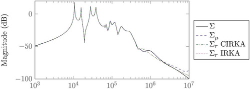
For all three cases considered, CIRKA required significantly less full-dimensional LU decompositions compared to IRKA. This is reflected also in the significant speedup in reduction time, ranging from four to over 20 times faster than IRKA. Note that for the case $n=10$, IRKA did not converge within the maximum number of steps. On the other hand, CIRKA converges to a local optimum, hence reaching a lower relative approximation error. As the model represents an oscillatory system with weakly damped eigenfrequencies and many outputs, it is hard to approximate well with a low reduced order, as the relative approximation errors in Table 1 reflect. Nevertheless, a comparison of the reduced models in a Bode diagram shows a good approximation, as it is depicted in Figure 6 exemplary for the case $n=30$ and the 9^th output.

Figure 6. Reduction of the gyro model using CIRKA and IRKA ($n=30$, 9th output).

To analyse the dependency of the results in Table 1 from the initialization, Table 2 summarizes the results for initial frequencies and tangential directions corresponding to the mirrored eigenvalues with smallest magnitude and respective input/output residues of the full model $\mathrm{\Sigma }$. This choice of initial parameters is known to be advantageous [31,32], its computation can be performed efficiently for large-scale sparse models using iterative methods (cf. e.g. the MATLAB command eigs).

Table 2. Reduction results for the gyro model using eigs initialization.

	IRKA				CIRKA
$n$	$k_{{\mathcal{H}}_2}$	$n_{LU}$	$t/s$	${ϵ}_{{\mathcal{H}}_2}$	$k_{\mu }$	${\sum }^{k_{{\mathcal{H}}_2}}$	$n_{LU}$	$t/s$	${ϵ}_{{\mathcal{H}}_2}$	${\widetilde{ϵ}}_{{\mathcal{H}}_2}$
10	1	5	19	0.28	2	8	6	25	0.41	0.26
20	9	90	323	0.17	2	30	14	60	0.12	0.05
30	9	136	493	0.03	2	40	22	96	0.02	5.57e-3

Interestingly, for the case $n=10$, IRKA converged to the default tolerance in one step, requiring only 5 LU decompositions. As CIRKA required two iterations until convergence, the number of full-dimensional LU decomposition required were 6. In this special case, IRKA was faster than CIRKA. In addition, comparison of the relative ${\mathcal{H}}_2$ error indicates that IRKA converged to a better local minimum. A comparison with the respective result of Table 1 demonstrates that initialization of ${\mathcal{H}}_2$-optimal reduction can have a large impact on the optimization and the results. For the other two cases, the pattern is similar to what discussed so far. In particular, the speedup obtained through CIRKA is significant.

Comparing the values of ${ϵ}_{{\mathcal{H}}_{2}H2}$ in Tables 1 and 2, we see that the value for CIRKA may be below, above, or the same as the one for IRKA. In general, it is not possible to say which method is expected to yield a better approximation quality. Given identical initializations, often times IRKA and CIRKA will converge to the same local optimum, especially in the case of small number of inputs and outputs. However, as the optimization in CIRKA is based on a surrogate of the actual cost function, it may converge to a different (better or worse) local optimum. Note that neither in IRKA, nor in CIRKA, we have control over which local optimum will be found – we only hope to find a local optimum. This is why in [29], an approach to find the global optimum exploiting the Model Function framework is presented.

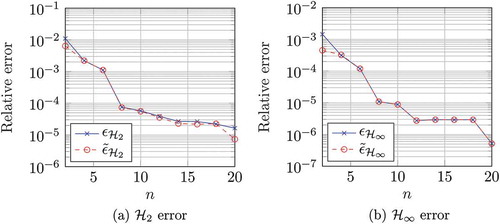
Finally, note that even when IRKA converges in few steps (e.g. 9) a reduction using CIRKA can already result in a significant speedup. Also note that the relative error estimation ${\widetilde{ϵ}}_{{\mathcal{H}}_2}$ tends to underestimate the approximation error, which has been observed especially for models with high dynamics. In general, it is not possible to state how far the estimate is from the real error. Nonetheless, given that no rigorous error bounds or estimators are yet available for ${\mathcal{H}}_2$-optimal reduction of general systems, we believe a non rigorous estimate at basically no additional cost may be of interest. To further investigate the validity of the error estimation based on the Model Function, Figure 11 compares the error estimations to the true error after reduction with CIRKA for the benchmark model CDplayer [21] and different reduced orders. Figure 7(a) shows the estimation of the ${\mathcal{H}}_2$ error as defined in (40), whereas in Figure 7(b) an analogous estimation of the ${\mathcal{H}}_{\mathrm{\infty }}$ error is given.

Figure 7. Comparison of relative error and its estimation for the CDplayer model.

6. Application to different system classes

The discussion of this contribution has been limited to the model reduction of linear time-invariant systems as in (1) with regular $E$ matrix. However, ${\mathcal{H}}_2$ approximation approaches exist for other system classes as well, including systems of Differential Algebraic Equations (DAEs) [33], systems for which only transfer function evaluations or measurements are available [19], linear systems with time delays [34], linear systems in port-Hamilton form [35], as well as non-linear systems in bilinear [36,37] or quadratic-bilinear form [38]. Obviously, going into the details of all approximation methods above would exceed the scope of this paper. Nonetheless, as we feel that ${\mathcal{H}}_2$ algorithms for different system classes could also benefit from the framework presented in this contribution, we will give brief indications of what steps and considerations are required to extend this framework. Generally speaking, the idea of surrogate optimization is certainly not new. However, as most methods above are based on interpolation, an update of the surrogate model as presented here can ensure interpolation of the full model with respect to optimal interpolation data, which would be otherwise lost. Once more, we emphasize that the idea presented in this contribution truly is a general framework and not just an additional reduction algorithm by the name of CIRKA. In the following, we briefly indicate for some system classes, how the principle of this new framework could be applied. The goal is to reduce the computational cost while still satisfying the same conditions as the original algorithms. Due to the brevity of the following subsections, readers who are not familiar with the system classes mentioned might prefer to skip these discussions.

6.1. DAE systems

DAE systems are state-space representations as in (1) having a singular matrix $E$. Their transfer function can be generally decomposed into the sum of a strictly proper part $G_{sp}(s)$, satisfying $\underset{s\to \mathrm{\infty }}{lim}{G}_{sp}(s)=0$, and a polynomial part $P(s)$, a polynomial in $s$ of order at most $\nu$, the so called index of the DAE [39]. Due to this polynomial contribution, approximation by tangential interpolation is not sufficient to prevent the reduction error to become unbounded, which is a result of a mismatch in the polynomial part. For this reason, in the reduction the polynomial part needs to be matched exactly, while the strictly proper part can be approximated through tangential interpolation. To achieve tangential interpolation of the strictly proper part while preserving the polynomial part, the subspace conditions in (4), (5) can be adapted by including spectral projectors onto deflating subspaces [33, Theorem 3.1]. Based on this, Gugercin, Stykel and Wyatt show in [33, Theorem 4.1] that interpolatory ${\mathcal{H}}_2$-optimal reduction of DAEs can be performed by using the modified subspace conditions to find an ${\mathcal{H}}_2$ approximation to the strictly proper part $G_{sp}(s)$.

For this system class, an extension of the Model Function framework is quite straightforward: By computing a Model Function following the modified interpolatory subspace conditions of [33, Theorem 3.1], ${\mathcal{H}}_2$ optimization can be performed on the surrogate instead of on the original DAE. An update of the Model Function finally leads to a reduced-order model that tangentially interpolates the strictly proper part of the original DAE at the optimal frequencies, along the optimal right and left tangential directions.

6.2. Port-Hamiltonian systems

Port-Hamiltonian (pH) formulations of linear dynamical systems are a very effective way to model systems that result from the interconnection of different subsystems, especially in a multi-physics domain. Their representation is similar to (1), where the system matrices have the special structures $E=I$, $A=(J-R)Q$, and $C=B^{\mathrm{T}}Q$, $J$ being a skew-symmetric interconnection matrix, $R$ a positive semi-definite dissipation matrix and $Q$ a positive definite energy matrix [40]. Models in pH form bear several advantages, such as passivity, and it is therefore of great relevance to preserve the pH structure after reduction. In a setting of tangential interpolation, this can be achieved by computing a projection matrix V according to (4) and choosing $W$ in order to retain the pH structure (cf [35,41].).

Gugercin, Polyuga, Beattie and van der Schaft present in [35] an iterative algorithm by the name of IRKA-PH, that adaptively chooses interpolation frequencies and input tangential directions, inspired by the IRKA iteration. In general, the resulting reduced model will not satisfy the first-order optimality conditions (17), as $W$ is not chosen to enforce bitangential Hermite interpolation but rather structure preservation. Nonetheless, the algorithm has shown to produce good approximations in practice.

To reduce the cost involved in repeatedly computing the projection matrices (4) in IRKA-PH, a Model Function in pH form could be introduced and updated. At convergence, the reduced model satisfies the condition (18) while being of pH-form as in the IRKA-PH case. In addition, the resulting Model Function (also in pH form) could be used e.g. for error estimation.

6.3. TF-IRKA

Gugercin and Beattie demonstrate in [19] how to construct a reduced-order model $G_r(s)$ satisfying first-order ${\mathcal{H}}_2$ optimality conditions (17) only from evaluations of the transfer function $G(s)$. The algorithm by the name of TF-IRKA exploits the Loewner-Framework, a data-driven approximation approach by Mayo and Antoulas [42] that produces a reduced model that tangentially interpolates the transfer function of a given system, whose transfer behaviour can be measured or evaluated at selected frequencies. Therefore, this algorithm can be used to obtain a reduced-order model satisfying optimality conditions for irrational, infinite dimensional dynamical systems for which an expression for $G(s)$ can be obtained by direct Laplace transformation of the partial differential equation, i.e. without prior discretization. In addition, it can be used for optimal approximation of systems where no model is available but the transfer behaviour $G(s)$ can be measured in experiments. Similar approaches have been derived to obtain reduced-order models for systems with delays [43].

The cost of TF-IRKA is dominated by the evaluation of the transfer function $G(s)$. In general, if an analytic expression is given, this cost is minimal compared to evaluating a discretized high-order model. However, if the evaluation is obtained through costly measurements, an approach to reduce the number of evaluations would be highly beneficial. In [44], Beattie, Drma$\stackrel{⌣}{\mathrm{c}}$, and Gugercin introduce a quadrature-based version of TF-IRKA for SISO models, called Q-IRKA, that only requires the evaluation of $G(s)$ once for some frequencies (quadrature nodes) and returns a reduced-order model that satisfies the optimality conditions (17) within the quadrature error. In [45], the same authors propose a similar approach by the name of QuadVF, based on vector fitting rational approximations using frequency sampling points.

By exploiting the new framework presented in this paper, it is possible to reduce the number of evaluations of $G(s)$ and satisfy the optimality conditions (17) exactly. By creating a surrogate using the Loewner-Framework, standard IRKA can be applied to obtain a new set of frequencies and tangential directions. Evaluating (or measuring) $G(s)$ for the new optimal frequencies allows to update the surrogate and repeat the process. Compared to Q-IRKA, this approach bears the additional advantage of automatically finding the amount and position of suitable frequencies for evaluating $G(s)$. In contrast, Q-IRKA and QuadVF require the initial evaluation of $G(s)$ at some pre-specified quadrature nodes. While a judicious spacing of the sampling frequencies in QuadVF was presented in [45], the frequency range and number of sampling points remains a tunable parameter within this approach.

6.4. Nonlinear systems

Model reduction approaches for general non-linear systems typically differ from what discussed in this contribution. However, in the case of weak nonlinearities, a bilinear formulation can be obtained by means of Carleman Bilinearization [46]. For this class of non-linear systems, the dynamic equations are similar to (1) and are complemented by an additional term that sums the weighted product between the state and the inputs. Recently, Benner and Breiten have presented in [36] a Bilinear IRKA (B-IRKA) algorithm that produces a reduced bilinear model satisfying, at convergence, first-order optimality conditions with respect to the bilinear ${\mathcal{H}}_2$ norm for the approximation error. This algorithm requires the repeated solution of two bilinear Sylvester equations, which can be obtained either by vectorization, solving linear systems of the dimension $Nn$, or, equivalently, computing the limit to an infinite series of linear Sylvester equations. Flagg and Gugercin have demonstrated in [37,47] for SISO models that the optimality conditions in [36] can be interpreted as interpolatory conditions of the underlying Volterra series ([37, Theorem 4.2]). In addition, they present an algorithm to construct reduced bilinear models that achieve multipoint Volterra series interpolation by construction (cf. [37, Theorem 3.1]), requiring the solution of two bilinear Sylvester equations. Exploiting the often fast convergence of the Volterra integrals, they propose a Truncated B-IRKA (TB-IRKA) that satisfies the first-order optimality conditions asymptotically as the truncation index tends to infinity. Note that extensions to bilinear DAEs were presented by Benner and Goyal in [48].

The interpolatory nature of this ${\mathcal{H}}_2$ approach makes it possible to extend the new framework presented in this paper to bilinear systems, hopefully speeding up the reduction with B-IRKA significantly. In fact, given a set of initial frequencies, a bilinear Model Function can be constructed that interpolates the Volterra series at these frequencies. This would require the solution of the full bilinear Sylvester equations for a few selected frequencies. Using this bilinear surrogate model, B-IRKA can be run efficiently on a lower dimension to find a new set of optimal frequencies and update the Model Function. Note that the cost of solving a full-dimensional bilinear Sylvester equation plays the same role in the complexity of B-IRKA as the cost of a full-dimensional LU decomposition for linear systems. Assuming the convergence behaviour of the new framework is similar to the linear case, this could lead to an algorithm that produces reduced bilinear models that satisfy the ${\mathcal{H}}_2$ optimality conditions exactly – i.e. without truncation error – at a far lower cost.

In presence of strong nonlinearities, the dynamics can be captured exactly in a quadratic bilinear model where, in addition, a quadratic term in the state variable is present. An ${\mathcal{H}}_2$ approach for this system class has been recently presented by Benner, Goyal and Gugercin in [38] and it is not evident at this point, how the new framework could be applied to this system class while preserving rigor of the results.

7. Conclusions and outlook

In this paper, we have presented a new general framework for ${\mathcal{H}}_2$-optimal reduction, based on the local nature of (tangential) interpolation and ${\mathcal{H}}_2$ optimality. The motivation to develop this framework, which can be interpreted e.g. as a surrogate optimization or subspace acceleration approach, has resulted from theoretical and numerical considerations on the cost of ${\mathcal{H}}_2$-optimal reduction. By means of updated surrogate optimization, the cost of reduction can be decoupled from the cost of optimization. Through a numerical example, we have illustrated the effectiveness of the new framework in reducing the cost of ${\mathcal{H}}_2$-optimal reduction. Theoretical considerations have demonstrated how the reduced-order models resulting from this new framework still satisfy first-order optimality conditions at convergence. The system class discussed in detail in this contribution has been MIMO LTI models. In addition, first indications have been given on how to extend this new framework for ${\mathcal{H}}_2$ reduction of different system classes, e.g. DAEs and bilinear systems. The new framework not only produces optimal reduced models at a far lower cost than conventional methods, but also provides – at no additional cost – a middle-sized surrogate model that can be used e.g. for error estimation, as demonstrated in numerical examples.

Recent research endeavours exploit the new framework to obtain the global optimum amongst all local ${\mathcal{H}}_2$ optimal reduced models of prescribed order [29]. In current research, the Model Function is used for error estimation in the cumulative reduction framework CURE by Panzer, Wolf and Lohmann [11,12,49] to adaptively chose the reduced order. Finally, the Model Function framework is currently being used in parametric model reduction to recycle the Model Function from one parameter sample point to another and reduce the cost tied to the repeated reduction at several points in the parameter space. Preliminary work is available in [50]. These advances will be topics of future investigations and publications.

Disclosure statement

No potential conflict of interest was reported by the authors.

Additional information

Funding

The work related to this contribution is supported by the German Research Foundation (DFG), Grant [LO408/19-1].

Notes

1. For dense matrices, this can be motivated by simple asymptotic operation counts. The QR decomposition of a $V\in {\mathbb{R}}^{N\times n}$ matrix via Householder requires $2n^2\left(N-\frac{n}{3}\right)$ flops and is hence linear in $N$. The flops involved in the product $W^{\mathrm{T}}EV$ are $nN(2N-1)+n^2(2N-1)$ for a dense $E$ and hence quadratic in $N$. Note however that for a diagonal $E$ matrix – an ideally sparse invertible matrix – the flops become at most $nN+n^2(2N-1)$, hence being linear in $N$ [23].

2. For the results of this contribution, we have used sparse LU decompositions, which are still feasible for models of relative large size even on standard machines (cf. Figure 1). This approach bears the advantage of allowing the recycling of LU factors, e.g. to solve LSEs with same left-hand sides. If other methods are used instead, some of the values and statements in this contribution may vary. Note, in addition, that complex conjugated pairs of shifts ${\sigma }_i=\overline{{\sigma }_j}$ yield complex conjugated directions $V_i^P=\overline{V_j^P}$. Therefore, the actual number of LSE to be solved may actually vary, making $2n$ a worst-case estimate.

3. All numerical examples presented in this contribution were generated using the sss and sssMOR toolboxes in MATLAB® [24].

References

- T. Penzl, A cyclic low-rank Smith method for large sparse Lyapunov equations, SIAM J. Sci. Comput. 21 (4) (2000), pp. 1401–1418. doi:10.1137/S1064827598347666
- V. Druskin, V. Simoncini, and M. Zaslavsky, Adaptive tangential interpolation in rational Krylov subspaces for MIMO dynamical systems, SIAM J. Matrix Anal. Appl. 35 (2) (2014), pp. 476–498. doi:10.1137/120898784
- P. Kürschner, Efficient low-rank solution of large-scale matrix equations, Ph.D. thesis, Max Planck Institute for Dynamics of Complex Technical Systems, 2016.
- E.J. Grimme, Krylov projection methods for model reduction, Ph.D. Thesis, University of Illinois at Urbana-Champaign, USA, 1997.
- C.A. Beattie and S. Gugercin, Model reduction by rational interpolation, in Model Reduction and Approximation: Theory and Algorithms, P. Benner, A.M. Cohen, M. Ohlberger, eds., et al., math.NA. SIAM, Sep. 2017, Available at http://arxiv.org/abs/1409.2140v1.
- K. Glover, All optimal Hankel-norm approximations of linear multivariable systems and their L∞-error norms, Int. J. Control 39 (6) (1984), pp. 1115–1193. doi:10.1080/00207178408933239
- A. Castagnotto, C.A. Beattie, and S. Gugercin, Interpolatory methods for H2∞ model reduction of multi-input/multi-output systems, in Model Reduction of Parametrized Systems, P. Benner, M. Ohlberger, A. Patera, eds., et al., Vol. 17, Modeling, Simulation & Applications, Springer, Cham, 2017, Chap. 22, pp. 349–365. doi:10.1007/978-3-319-58786-8_22
- S. Gugercin, A.C. Antoulas, and C.A. Beattie, H2 model reduction for largescale dynamical systems, SIAM J. Matrix Anal. Appl. 30 (2) (2008), pp. 609–638. doi:10.1137/060666123
- P. Van Dooren, K. Gallivan, and P.-A. Absil, H2-optimal model reduction of MIMO systems, Appl. Math. Lett. 21 (2008), pp. 1267–1273. doi:10.1016/j.aml.2007.09.015
- C.A. Beattie and S. Gugercin, A trust region method for optimal H2 model reduction, in IEEE Conference on Decision and Control, IEEE, 2009, pp. 5370–5375. doi:10.1109/CDC.2009.5400605
- H.K.F. Panzer, S. Jaensch, T. Wolf, et al. A Greedy Rational Krylov Method for H2-pseudooptimal model order reduction with preservation of stability, in Proceedings of the American Control Conference, 2013, pp. 5512–5517.
- H.K.F. Panzer, Model order reduction by Krylov subspace methods with global error bounds and automatic choice of parameters, Ph.D. thesis, Technische Universität München, 2014.
- A. Castagnotto, H.K.F. Panzer, and B. Lohmann, Fast H2-optimal model order reduction exploiting the local nature of Krylov-subspace methods, in European Control Conference 2016, Aalborg, Denmark, 2016, pp. 1958–1963. doi:10.1109/ECC.2016.7810578
- K. Gallivan, A. Vandendorpe, and P. Van Dooren, Model reduction of MIMO systems via tangential interpolation, SIAM J. Matrix Anal. Appl. 26 (2) (2004), pp. 328–349. doi:10.1137/S0895479803423925
- K. Gallivan, A. Vandendorpe, and P. Van Dooren, Sylvester equations and projection-based model reduction, J. Comput. Appl. Math. 162 (1) (2004), pp. 213–229. doi:10.1016/j.cam.2003.08.026
- A.C. Antoulas, Approximation of Large-Scale Dynamical Systems, Vol. 6, Advances in Design and Control, SIAM Publications, Philadelphia, PA, 2005, ISBN 9780898715293. doi:10.1137/1.9780898718713
- A.C. Antoulas, C.A. Beattie, and S. Gugercin, Interpolatory model reduction of large-scale dynamical systems, in Efficient Modeling and Control of Large-Scale Systems, Springer US, 2010, pp. 3–58. doi:10.1007/978-1-4419-57573_1
- L. Meier and D.G. Luenberger, Approximation of linear constant systems, IEEE Trans. Autom. Control 12 (5) (Oct., 1967), pp. 585–588. doi:10.1109/TAC.1967.1098680
- C.A. Beattie and S. Gugercin, Realization-independent H22-approximation, in 51st IEEE Conference on Decision and Control, IEEE, 2012, pp. 4953–4958. doi:10.1109/CDC.2012.6426344
- Y. Saad, Iterative Methods for Sparse Linear Systems, SIAM, 2003.
- Y. Chahlaoui and P. Van Dooren, A collection of benchmark examples for model reduction of linear time invariant dynamical systems, Tech. rep. 2002-2, SLICOT Working Note, 2002. Available at www.slicot.org.
- J.G. Korvink and E.B. Rudnyi, Oberwolfach benchmark collection, in Dimension Reduction of Large-Scale Systems, P. Benner, D.C. Sorensen, and V. Mehrmann, eds., Vol. 45, Lecture Notes in Computational Science and Engineering, Springer Berlin Heidelberg, 2005, pp. 311–315. doi:10.1007/3-54027909-1_11
- G.H. Golub and C.F. Van Loan, Matrix Computations, Johns Hopkins University Press, Baltimore, 1996.
- A. Castagnotto, M. Cruz Varona, and L. Jeschek, sss & sssMOR: analysis and reduction of large-scale dynamic systems in MATLAB, atAutomatisierungstechnik, 65 (2) (2017), pp. 134–150. doi:10.1515/auto-20160137
- N.V. Queipo, R.T. Haftka, W. Shyy, T. Goel, R. Vaidyanathan, and P. Kevin Tucker, Surrogate-based analysis and optimization, Prog. Aerosp. Sci. 41 (1) (2005), pp. 1–28. doi:10.1016/j.paerosci.2005.02.001
- P. Benner, Z. Tomljanović, and N. Truhar, Optimal damping of selected eigenfrequencies using dimension reduction, Numer. Lin. Alg. Appl. 20 (1) (2013), pp. 1–17, ISSN . doi:10.1002/nla.833
- J. Rommes and N. Martins, Effcient computation of transfer function dominant poles using subspace acceleration, IEEE Trans. Power Syst. 21 (4) (2006), pp. 1218–1226. doi:10.1109/TPWRS.2006.876671
- J.D. Pintér, Global Optimization in Action: Continuous and Lipschitz Optimization: Algorithms, Implementations and Applications, Vol. 6, Springer Science & Business Media, 2013.
- A. Castagnotto, S. Hu, and B. Lohmann, An approach for globalized H2-optimal model reduction, in Proceedings of the 9th Vienna International Conference on Mathematical Modelling, 2018.
- J. Lienemann, D. Billger, E.B. Rudnyi, et al., MEMS compact modeling meets model order reduction: Examples of the application of Arnoldi methods to microsystem devices, in The Technical Proceedings of the 2004 Nanotechnology Conference and Trade Show, Nanotech, Vol. 4, 2004.
- S. Gugercin, Projection methods for model reduction of large-scale dynamical systems, Ph.D. thesis, Rice University, 2003. Available at http://hdl.%20handle.%20net/1911/18536.
- S. Gugercin and A.C. Antoulas, An H2 error expression for the Lanczos procedure, in 42nd IEEE Conference on Decision and Control, Vol. 2, IEEE, 2003, pp. 1869–1872.
- S. Gugercin, T. Stykel, and S. Wyatt, Model reduction of descriptor systems by interpolatory projection methods, SIAM J. Sci. Comput. 35 (5) (2013), pp. B1010–B1033. doi:10.1137/130906635
- I. Pontes Duff, S. Gugercin, C. Beattie, C. Poussot-Vassal, and C. Seren, H2-optimality conditions for reduced time-delay systems of dimension one, IFAC Pap. OnLine 49 (10) (2016), 13th IFAC Workshop on Time Delay Systems TDS 2016, pp. 7–12. doi:10.1016/j.ifacol.2016.07.464
- S. Gugercin, R.V. Polyuga, C. Beattie, and A. van der Schaft, Structure-preserving tangential interpolation for model reduction of port-Hamiltonian systems, Autom. 48 (9) (2012), pp. 1963–1974. doi:10.1016/j.automatica.2012.05.052.
- P. Benner and T. Breiten, Interpolation-based H2-model reduction of bilinear control systems, SIAM J. Matrix Anal. Appl. 33 (3) (2012), pp. 859–885. doi:10.1137/110836742
- G.M. Flagg and S. Gugercin, Multipoint volterra series interpolation and H2Optimal model reduction of bilinear systems, SIAM J. Numer. Anal. 36 (2) (2015), pp. 549–579. doi:10.1137/130947830
- P. Benner, P. Goyal, and S. Gugercin, H2-quasi-optimal model order reduction for quadratic-bilinear control systems, arXiv Preprint arXiv:1610.03279 (2016).
- P. Benner and T. Stykel, Model Order Reduction for Differential-Algebraic Equations: A Survey, Springer, 2017, pp. 107–160.
- A. van der Schaft, L2-Gain and Passivity Techniques in Nonlinear Control, 3rd ed., Springer, 2017.
- T. Wolf, B. Lohmann, R. Eid, and P. Kotyczka, Passivity and structure preserving order reduction of linear port-Hamiltonian systems using Krylov subspaces, Eur. J. Control 16 (4) (2010), pp. 401–406. doi:10.3166/ejc.16.401-406
- A.J. Mayo and A.C. Antoulas, A framework for the solution of the generalized realization problem, Linear Algebra Appl. 425 (2–3) (2007), Special Issue in honor of P. A. Fuhrmann, Edited by A. C. Antoulas, U. Helmke, J. Rosenthal, V. Vinnikov, and E. Zerz, pp. 634–662, ISSN: . doi:10.1016/j.laa.2007.03.008
- I. Pontes Duff, C. Poussot-Vassal, and C. Seren, Realization independent single time-delay dynamical model interpolation and H2-optimal approximation, in 2015 54th IEEE Conference on Decision and Control (CDC), Dec. 2015, pp. 4662–4667. doi:10.1109/CDC.2015.7402946
- C. Beattie, Z. Drmač, and S. Gugercin, Quadrature-based IRKA for optimal H2 model reduction, IFAC Pap. OnLine 48 (1) (2015), 8th Vienna International Conferenceon Mathematical Modelling, pp. 5–6. doi:10.1016/j.ifacol.2015.05.196.
- Z. Drmač, S. Gugercin, and C. Beattie, Quadrature-based vector fitting for discretized H2 approximation, SIAM J. Sci. Comput. 37 (2) (2015), pp. A625–A652. doi:10.1137/140961511
- W.J. Rugh, Nonlinear System Theory, Johns Hopkins University Press Baltimore, 1981.
- G.M. Flagg, Interpolation methods for the model reduction of bilinear systems, Ph.D. Thesis, Virginia Polytechnic Institute and State University, Blacksburg, Virginia, Apr. 2012.
- P. Benner and P. Goyal, Multipoint interpolation of volterra series and H2Model reduction for a family of bilinear descriptor systems, Syst. Control Lett. 97 (2016), pp. 1–11. doi:10.1016/j.sysconle.2016.08.008
- T. Wolf, Pseudo-optimal model order reduction, Dissertation, Technische Universität München, Munich, Germany, 2015.
- J. Peters, Parametrische modellordnungsreduktion mit dem H2-optimalen Modellfunktions-Framework, Bachelor Thesis, Technical University of Munich, Oct. 2017.