Port-Hamiltonian fluid–structure interaction modelling and structure-preserving model order reduction of a classical guitar

ABSTRACT

A fluid–structure interaction model in a port-Hamiltonian representation is derived for a classical guitar. After discretization, we combine the laws of continuum mechanics for solids and fluids within a unified port-Hamiltonian (pH) modelling approach by adapting the equations through an appropriate coordinate transformation on the second-order level. The high-dimensionality of the resulting system is reduced by model order reduction. The article focuses on pH-systems in different state transformations, a variety of basis generation techniques as well as structure-preserving model order reduction approaches that are independent from the projection basis. As main contribution, a thorough comparison of these method combinations is conducted. In contrast to typical frequency-based simulations in acoustics, transient time simulations of the system are presented. The approach is embedded into a straightforward workflow of sophisticated commercial software modelling and flexible in-house software for multi-physics coupling and model order reduction.

KEYWORDS:

• structure-preserving model order reduction
• port-Hamiltonian systems
• fluid–structure interaction
• classical guitar

1. Introduction

For the development of sophisticated products and the understanding of complex technical systems, the modelling and simulation of these is essential. The consideration of different involved physical phenomena is indispensable for a realistic representation but also poses new challenges in the description of the variables and a reasonable coupling. The port-Hamiltonian (pH) representation is based on the idea of interconnecting Hamiltonian systems and including dissipation in the formulation, for this reason, the energy is used as the lingua franca at the coupling ports [1]. This approach is attracting increasing attention due to its ability to describe complex multi-physics systems in the context of automated modelling and provides the basis for a unified description of modelling, analysis, control, optimization, and model order reduction. Furthermore, under mild assumptions, pH-systems implicitly ensure important system properties such as passivity, stability and energy conservation [2,3].

Fluid–structure interaction (FSI) characterizes the interaction of a moving or deformable mechanical structure with an internal or surrounding fluid [4]. The consideration of FSI plays a crucial role in different applications, e.g. the bending of aircraft wings, the blood flow in large veins or the lubricant flow in ball-bearings [5]. In the current study, we want to analyse an acoustic system in which FSI is also of great importance for its proper technical function.

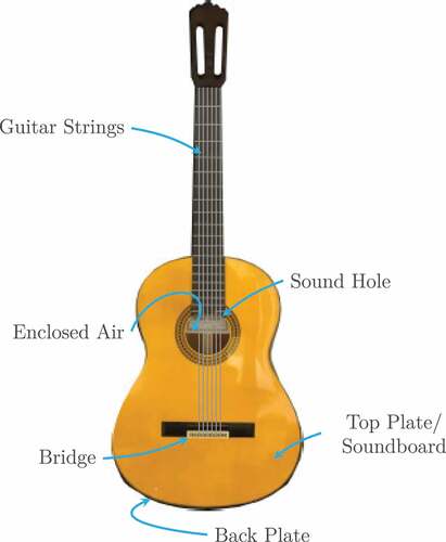
A classical guitar is a popular instrument consisting of various components whose most important ones are briefly described in order to understand the physical context of the mathematical problem, see Figure 1. The musician plucks the guitar strings which thereupon start to vibrate. Those vibrations are transferred through the bridge into the soundboard which is the top plate of the guitar body. The guitar body coupled with the enclosed air acts as a resonator for the strings’ vibration. The guitar’s composition and material properties influence the volume and timbre of the air escaping through the sound hole.

Figure 1. Classical guitar.

The classical guitar represents an impressive example of a multi-physics system where the guitar body is strongly coupled with the enclosed air and the coupling effects cannot be neglected for a realistic representation of the behaviour. The modelling of a guitar without strings can be found, e.g., in [6–8] and the modelling of strings in [9,10]. Numerical simulations of a coupled guitar model were performed in [11,12]. Port-Hamiltonian representations of acoustic models are presented for instance in [13] for the vocal apparatus and for a Rhodes piano in [14]. The modelling procedure of this work follows closely the approach presented in [6].

In the current study, this FSI problem is derived from the partial differential equation of linear elasticity for the mechanical structure [15] and the wave equation for the fluid [16]. The system is spatially discretized with the finite element (FE) method in order to obtain a coupled second-order ordinary differential equation (ODE) system [17]. Structural damping obtained from measurements is included into the model [6]. From this basis, a port-Hamiltonian representation is attained by first transforming the system into a first-order system and then applying an adapted state transformation. The coupling effects of the multi-domain system are illustrated in a transient time simulation which gives further insight into classical frequency-based analyses in acoustics.

The spatial discretization via FE methods typically leads to high-dimensional systems that are ill-suited for multi-query simulations, e.g. for usage in optimization loops. Hence, model order reduction (MOR) methods are essential to approximate the system in a subspace of a much lower dimension for a faster and more efficient simulation [18]. One major novelty is the presentation of a comprehensive sensitivity analysis for a variety of combinations of projection methods and basis generation methods, i.e. the calculation of projection matrices, for reducing the FSI problem. The projection methods focus on basis-independent structure-preserving¹ reduction [19,20] to preserve the important system properties in comparison to non-structure-preserving variants. The basis generation comprises approaches that are based on the system matrices, such as modal truncation [18,21] or moment-matching via Krylov subspaces [22], and data-based techniques based on time-response snapshots, e.g. Proper Orthogonal Decomposition (POD) [23] and Proper Symplectic Decomposition (PSD) [24,25]. For more information on recent developments in structure-preserving MOR procedures for both Hamiltonian and port-Hamiltonian systems, we refer to [26–29] and the references therein.

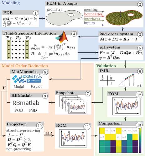
The paper is organized as follows. In Section 2, the dynamic equations for a fluid–structure interaction problem are derived and adapted on second-order level. Additionally, practical aspects from the enhanced modelling process as an ensemble between the commercial software Abaqus and in-house code in Matlab are described. In Section 3, the necessary background on port-Hamiltonian systems is given and the FSI model of the guitar in a port-Hamiltonian input-output state representation is derived. Based on this, further pH formulations are deduced and the transient time simulation of the full system is performed. Various non-common projection methods, both structure-preserving and non-structure-preserving, are presented in Section 4. In Section 5, we recall classical and introduce modern basis generation methods with adapted snapshot matrices and non-orthogonal bases. The comprehensive sensitivity analysis is given in Section 6. Finally, we conclude the paper. An overview of the entire workflow is given in Figure 2. In the remainder, this workflow diagram will be referenced by a circled number which highlights the workflow area the current section is referring to, e.g. ①.

Figure 2. Workflow diagram.

2. Modelling of a classical guitar

When producing a tone with a guitar, many different guitar components interact with each other, with the interaction of the guitar body and enclosed air being of particular importance. An enhanced three mass model focuses on this interaction and serves as a comprehensive system on which the investigated methodologies are presented. The present chapter first describes the mathematical background of this fluid–structure interaction and then also addresses the practical aspects of its implementation using Abaqus and Matlab.

2.1. Derivation of the dynamic equations for the fluid–structure interaction

The vibration of the mechanical structure can be described as an elastic motion of the wooden plates of the guitar that can be mathematically explained by the methods of continuum mechanics, cf. ①. The motion of a body is described by the motion of all material points ${\mathcal{P}}_S$ for this body, where the current position of each point can be classified by its position ${\mathit{R}}_0$ in the initial configuration and the displacement $\mathit{z}({\mathit{R}}_0,t)$. Assuming small strains leads to the elastodynamic problem for the time interval $I_t=[0,t_{\mathrm{e}\mathrm{n}\mathrm{d}}]$

(1a) $\mathrm{f}\mathrm{o}\mathrm{r}\mathrm{c}\mathrm{e}\mathrm{e}\mathrm{q}\mathrm{u}\mathrm{i}\mathrm{l}\mathrm{i}\mathrm{b}\mathrm{r}\mathrm{i}\mathrm{u}\mathrm{m}:{\rho }_S\stackrel{..}{\mathit{z}}=\mathrm{\nabla }\cdot \sigma (\mathit{z})+{\mathit{b}}_0,\mathrm{i}\mathrm{n}{I}_t\times {\mathcal{P}}_S$(1a)

(1b) $\mathrm{b}\mathrm{o}\mathrm{u}\mathrm{n}\mathrm{d}\mathrm{a}\mathrm{r}\mathrm{y}\mathrm{c}\mathrm{o}\mathrm{n}\mathrm{d}\mathrm{i}\mathrm{t}\mathrm{i}\mathrm{o}\mathrm{n}:\mathit{z}={\mathit{z}}_b,\mathrm{i}\mathrm{n}{I}_t\times {\mathrm{\Gamma }}_{\mathrm{z}}$(1b)

(1c) $\mathrm{c}\mathrm{o}\mathrm{u}\mathrm{p}\mathrm{l}\mathrm{i}\mathrm{n}\mathrm{g}\mathrm{t}\mathrm{e}\mathrm{r}\mathrm{m}:\sigma \mathbf{n}=\mathbf{t},\mathrm{i}\mathrm{n}{I}_t\times {\mathrm{\Gamma }}_{FSI}$(1c)

(1d) $\mathrm{s}\mathrm{t}\mathrm{r}\mathrm{a}\mathrm{i}\mathrm{n}-\mathrm{d}\mathrm{i}\mathrm{s}\mathrm{p}\mathrm{l}\mathrm{a}\mathrm{c}\mathrm{e}\mathrm{m}\mathrm{e}\mathrm{n}\mathrm{t}\mathrm{r}\mathrm{e}\mathrm{l}\mathrm{a}\mathrm{t}\mathrm{i}\mathrm{o}\mathrm{n}:{\epsilon }_s=\frac{1}{2}\left(\mathrm{\nabla }\mathbf{z}+{(\mathrm{\nabla }\mathbf{z})}^{\mathrm{\top }}\right),\mathrm{i}\mathrm{n}{\mathcal{P}}_S$(1d)

(1e) $\mathrm{c}\mathrm{o}\mathrm{n}\mathrm{s}\mathrm{t}\mathrm{i}\mathrm{t}\mathrm{u}\mathrm{t}\mathrm{i}\mathrm{v}\mathrm{e}\mathrm{e}\mathrm{q}\mathrm{u}\mathrm{a}\mathrm{t}\mathrm{i}\mathrm{o}\mathrm{n}(Hook{e}^{\prime }\mathrm{s}\mathrm{l}\mathrm{a}\mathrm{w}):\sigma ={\mathit{C}}_{\mathrm{E}\mathrm{M}}{\epsilon }_s,\mathrm{i}\mathrm{n}{\mathcal{P}}_S$(1e)

(1f) $\mathrm{i}\mathrm{n}\mathrm{i}\mathrm{t}\mathrm{i}\mathrm{a}\mathrm{l}\mathrm{c}\mathrm{o}\mathrm{n}\mathrm{d}\mathrm{i}\mathrm{t}\mathrm{i}\mathrm{o}\mathrm{n}:\mathit{z}={\mathit{z}}_0,\mathrm{i}\mathrm{n}{\mathcal{P}}_S$(1f)

(1g) $\begin{array}{rl}& \mathrm{i}\mathrm{n}\mathrm{i}\mathrm{t}\mathrm{i}\mathrm{a}\mathrm{l}\mathrm{c}\mathrm{o}\mathrm{n}\mathrm{d}\mathrm{i}\mathrm{t}\mathrm{i}\mathrm{o}\mathrm{n}:\mathbf{z}={\mathbf{z}}_0,\mathrm{i}\mathrm{n}{\mathcal{P}}_S\\ & \stackrel{.}{z}=\underset{0}{\overset{.}{z}},\mathrm{i}\mathrm{n}{\mathcal{P}}_S\end{array}$(1g)

known as the strong formulation. The fundamental laws and material-dependence are considered in the force equilibrium (1a)(1a) $\mathrm{f}\mathrm{o}\mathrm{r}\mathrm{c}\mathrm{e}\mathrm{e}\mathrm{q}\mathrm{u}\mathrm{i}\mathrm{l}\mathrm{i}\mathrm{b}\mathrm{r}\mathrm{i}\mathrm{u}\mathrm{m}:{\rho }_S\stackrel{..}{\mathit{z}}=\mathrm{\nabla }\cdot \sigma (\mathit{z})+{\mathit{b}}_0,\mathrm{i}\mathrm{n}{I}_t\times {\mathcal{P}}_S$(1a) and the constitutive equation (1e)(1e) $\mathrm{c}\mathrm{o}\mathrm{n}\mathrm{s}\mathrm{t}\mathrm{i}\mathrm{t}\mathrm{u}\mathrm{t}\mathrm{i}\mathrm{v}\mathrm{e}\mathrm{e}\mathrm{q}\mathrm{u}\mathrm{a}\mathrm{t}\mathrm{i}\mathrm{o}\mathrm{n}(Hook{e}^{\prime }\mathrm{s}\mathrm{l}\mathrm{a}\mathrm{w}):\sigma ={\mathit{C}}_{\mathrm{E}\mathrm{M}}{\epsilon }_s,\mathrm{i}\mathrm{n}{\mathcal{P}}_S$(1e) . The density of the material ${\rho }_S$, the second temporal derivative of the displacements $z$, the divergence of the stress tensor $\sigma$ and the volume forces ${\mathit{b}}_0$ form the force equilibrium (1a), where $\mathrm{\nabla }$ describes the nabla operator. The constitutive equation (1e)(1e) $\mathrm{c}\mathrm{o}\mathrm{n}\mathrm{s}\mathrm{t}\mathrm{i}\mathrm{t}\mathrm{u}\mathrm{t}\mathrm{i}\mathrm{v}\mathrm{e}\mathrm{e}\mathrm{q}\mathrm{u}\mathrm{a}\mathrm{t}\mathrm{i}\mathrm{o}\mathrm{n}(Hook{e}^{\prime }\mathrm{s}\mathrm{l}\mathrm{a}\mathrm{w}):\sigma ={\mathit{C}}_{\mathrm{E}\mathrm{M}}{\epsilon }_s,\mathrm{i}\mathrm{n}{\mathcal{P}}_S$(1e) involves the engineering strain ${\epsilon }_{\mathbf{s}}$ and elastic modulus ${\mathit{C}}_{\mathrm{E}\mathrm{M}}$. In (1a), $\mathrm{\nabla }\cdot \mathit{\sigma }(\mathit{z})$ denotes the row-wise divergence of the tensor $\sigma$ resulting in a vector. In (1d) the nabla operator gives rise to row and column vectors, whose addition is to be understood componentwise, resulting in a tensor. We restrict ourselves to the case of orthotropic, linear elastic material behaviour which can be parametrized with nine parameters: three Young’s moduli, three Poisson ratios and three shear moduli to consider the behaviour in each spatial direction [30]. $\mathrm{\Gamma }{ }_z$ describes the parts of the body surface where Dirichlet boundary conditions for the displacement ${\mathit{z}}_b$ apply, cf. Figure 4. Likewise, ${\mathrm{\Gamma }}_{FSI}$ describes the contact surface of the mechanical structure and the encased air on which the stresses are given by the surface traction $\mathit{t}=p{\mathit{n}}_{FSI}$ whose magnitude scales proportionally with the pressure $p$ of the air at the contact surface. Here ${\mathit{n}}_{FSI}$ denotes the normal vector of unit length pointing into the direction of the encased air. The initial conditions at time $t=0$ are given for the displacements ${\mathit{z}}_0$ and velocities ${\dot{\mathit{z}}}_0$ [15,17,31].

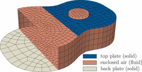
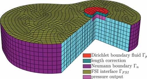
Figure 3. Sectional view of the FEM multi-physics model of a classical guitar.

For a numerical simulation, the continuum is spatially discretized with the finite element method (FEM) resulting in the symmetric mass matrix ${\mathit{M}}_S\in {\mathbb{R}}^{N_S\times N_S}$ and the symmetric stiffness matrix ${\mathit{K}}_S\in {\mathbb{R}}^{N_S\times N_S}$. To model dissipation effects, i.e. the damping parameters, we employ the so-called Rayleigh damping

(2) ${\mathit{D}}_S=\alpha {\mathit{M}}_S+\beta {\mathit{K}}_S$(2)

with the coefficients $\alpha$ and $\beta$. Measurements of the damping ratio were conducted on a real guitar at different frequencies ${\omega }_D$, see [6,32], and the overdetermined equation system is solved by using a least square fit for the coefficients that results in $\alpha =15.958\frac{1}{\mathrm{s}}$ and $\beta =2.821\cdot {10}^{-6}\mathrm{s}$. The coefficients describe the first two terms of the so-called Caughey series [33]. Higher-order terms are neglected since the results are already in good agreement with the measurements [6,32].

This complements the dynamic equation of the mechanical structure resulting in the second-order space discretized system, c.f. ③

(3) ${\mathit{M}}_S\ddot{\mathit{z}}+{\mathit{D}}_S\dot{\mathit{z}}+{\mathit{K}}_S\mathit{z}={\mathit{f}}_S+{\mathit{f}}_p$(3)

with the damping matrix ${\mathit{D}}_S\in {\mathbb{R}}^{N_S\times N_S}$ and the excitation forces ${\mathit{f}}_S,{\mathit{f}}_p\in {\mathbb{R}}^{N_S}$ for the mechanical structure, whereas the latter is the specific force stemming from the coupling term (1c).

The geometry and division of the guitar into the different domains can be seen in Figure 3. The model consists of three different parts: the top plate or soundboard with a sound hole, the back plate and the air inside the guitar body in the shape and of the size of a classical guitar. Modelling the guitar behaviour with these parts (in lumped parameter form) is known as a three mass model [7]. The approach of [6] is used as a reference to create an enhanced three mass model with the FEM, which will be discussed further in Section 2.2.

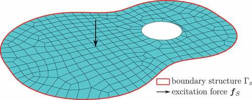
Figure 4. Meshed top plate.

(4a) $\mathrm{a}\mathrm{c}\mathrm{o}\mathrm{u}\mathrm{s}\mathrm{t}\mathrm{i}\mathrm{c}\mathrm{w}\mathrm{a}\mathrm{v}\mathrm{e}\mathrm{e}\mathrm{q}\mathrm{u}\mathrm{a}\mathrm{t}\mathrm{i}\mathrm{o}\mathrm{n}:\frac{1}{c_0^2}\frac{{\mathrm{\partial }}^{2}p}{\mathrm{\partial }{t}^2}-{\mathrm{\nabla }}^{2}p=0,\mathrm{i}\mathrm{n}{I}_t\times {\mathcal{P}}_F$(4a)

(4b) $\mathrm{b}\mathrm{o}\mathrm{u}\mathrm{n}\mathrm{d}\mathrm{a}\mathrm{r}\mathrm{y}\mathrm{c}\mathrm{o}\mathrm{n}\mathrm{d}\mathrm{i}\mathrm{t}\mathrm{i}\mathrm{o}\mathrm{n}\mathrm{s}:p=p_b,\mathrm{i}\mathrm{n}{I}_t\times {\mathrm{\Gamma }}_p$(4b)

(4c) $\frac{\mathrm{\partial }p}{\mathrm{\partial }\mathit{n}}=0,\mathrm{i}\mathrm{n}{I}_t\times {\mathrm{\Gamma }}_n$(4c)

(4d) $\text{coupling}\text{term}:\frac{\partial p}{\partial n_{FSI}}=-{\rho }_F{\left(\frac{{\partial }^{2}z}{\partial t^2}\right)}^{\top }{n}_{FSI},\text{in}{I}_t\times {\Gamma }_{FSI}$(4d)

(4e) $\text{initial}\text{conditions}:p=p_0,\text{in}{p}_{\mathrm{F}}$(4e)

(4f) $\stackrel{.}{p}={\stackrel{.}{p}}_0,\text{in}{p}_F$(4f)

The fluid behaviour, c.f. ①, can be described with where the acoustic wave equation is derived from the Euler equations for ideal, compressible fluids with Dirichlet boundary conditions $p_b\mathrm{o}\mathrm{n}{\mathrm{\Gamma }}_p$. The zero Neumann boundary conditions (4c) on ${\mathrm{\Gamma }}_n$ are used as a means to compensate the fact that we only model the top and bottom plate of the mechanical structure but not the sides. The force applied to the mechanical structure along the normal direction, i.e. $\frac{\mathrm{\partial }p}{\mathrm{\partial }{\mathit{n}}_{FSI}}$ is equal in magnitude but of opposite direction compared to the force applied by the mechanical structure along the normal direction, i.e. $-{\rho }_F{\left(\frac{{\mathrm{\partial }}^2\mathit{z}}{\mathrm{\partial }{t}^2}\right)}^{\mathrm{\top }}{\mathit{n}}_{FSI}$, where ${\rho }_F$ denotes the density of the fluid. The boundary domains of the fluid are visualized in Figure 5. The acoustic wave equation (4a)(4a) $\mathrm{a}\mathrm{c}\mathrm{o}\mathrm{u}\mathrm{s}\mathrm{t}\mathrm{i}\mathrm{c}\mathrm{w}\mathrm{a}\mathrm{v}\mathrm{e}\mathrm{e}\mathrm{q}\mathrm{u}\mathrm{a}\mathrm{t}\mathrm{i}\mathrm{o}\mathrm{n}:\frac{1}{c_0^2}\frac{{\mathrm{\partial }}^{2}p}{\mathrm{\partial }{t}^2}-{\mathrm{\nabla }}^{2}p=0,\mathrm{i}\mathrm{n}{I}_t\times {\mathcal{P}}_F$(4a) contains the speed of sound $c_0$ and the pressure $p$ on the domain ${\mathcal{P}}_F$ [16,34].

Figure 5. Meshed fluid.

The wave equation is spatially discretized by using the Galerkin method with linear shape functions. This leads, c.f. ③, to the dynamic equations of the fluid in matrix form [35]

(5) ${\mathit{M}}_F\ddot{\mathit{p}}+{\mathit{K}}_F\mathit{p}={\mathit{f}}_F+{\mathit{f}}_{\mathit{z}}$(5)

with the symmetric mass matrix ${\mathit{M}}_F\in {\mathbb{R}}^{N_F\times N_F}$, the symmetric stiffness matrix ${\mathit{K}}_F\in {\mathbb{R}}^{N_F\times N_F}$, the excitation vector for the fluid ${\mathit{f}}_F\in {\mathbb{R}}^{N_F}$ and the excitation vector ${\mathit{f}}_{\mathit{z}}\in {\mathbb{R}}^{N_F}$ stemming from the interaction with the mechanical structure, i.e. the coupling term (4d).

FSI is an area that describes the multi-physics coupling between the domains of fluid dynamics and structural mechanics. The coupling is considered a strong FSI if the motion of the solid influences the fluid and vice versa [34]. The classical guitar as the studied system allows the investigation of these strong couplings. In our case, this coupling is expressed via the coupling terms (1c) and (4d).

The effects of the mechanical structure on the fluid and vice versa, c.f. ④, result in the external forces ${\mathit{f}}_p$ and ${\mathit{f}}_{\mathit{z}}$, respectively. The former relates to the force

(6) $f_p\widehat{=}{\displaystyle {\int }_{{\Gamma }_{FSI}}{t}^T}zdA={\displaystyle {\int }_{{\Gamma }_{FSI}}p}{z}^T{n}_{FSI}dA$(6)

induced by the surface traction $\mathit{t}$. The latter corresponds to the force

(7) ${\mathit{f}}_{\mathit{z}}\hspace{0.17em}\widehat{=}{\int }_{{\mathrm{\Gamma }}_{FSI}}-{\rho }_F{\left(\frac{{\mathrm{\partial }}^2\mathit{z}}{\mathrm{\partial }{t}^2}\right)}^{\mathrm{\top }}{\mathit{n}}_{FSI}pdA$(7)

generated by the acceleration of the mechanical structure along the normal direction ${\left(\frac{{\mathrm{\partial }}^2\mathit{z}}{\mathrm{\partial }{t}^2}\right)}^{\mathrm{\top }}{\mathit{n}}_{FSI}$ . Hence, both ${\mathit{f}}_p$ and ${\mathit{f}}_{\mathit{z}}$ can be represented as a matrix vector product

(8) ${\mathit{f}}_p=\mathit{R}p\mathrm{a}\mathrm{n}\mathrm{d}{\mathit{f}}_{\mathit{z}}=-{\rho }_F{\mathit{R}}^{\mathrm{\top }}\ddot{\mathit{z}}$(8)

where $\mathit{R}$ describes the coupling matrix [35] representing the term

(9) $\mathit{R}\hspace{0.17em}\widehat{=}{\int }_{{\mathrm{\Gamma }}_{FSI}}p{\mathit{z}}^{\mathrm{\top }}{\mathit{n}}_{FSI}\mathrm{d}A.$(9)

However, in the present case of non-matching meshes, the nodal values of the acoustic and structural domains, which are part of the interface, are related to each other with linear interpolation.

For each node in the structural domain we identify the corresponding mesh-element of the acoustic domain in which the structural node is located. We then compute the barycentric coordinates of this node and distribute the effect of the interaction by the proportions corresponding to the barycentric coordinates.

Consequently, the separate equations for the mechanical structure (3) and the fluid (5) can be combined into the following coupled system

(10) $\left[M_S{0}_{{\rho }_F}{R}^T{M}_F\right]\widehat{M}\$\$\in ℝ\widehat{N}\widehat{N}\left[\stackrel{\mathrm{..}}{z}\stackrel{\mathrm{..}}{p}\right]\stackrel{\mathrm{..}}{\widehat{x}}\in ℝ\widehat{N}+\left[D_{S}000\right]\widehat{D}\in ℝ\widehat{N}\widehat{N}\left[\stackrel{.}{z}\stackrel{.}{p}\right]\stackrel{.}{\widehat{x}}\in ℝ\widehat{N}+\left[K_S-R0K_F\right]\widehat{K}\in ℝ\widehat{N}\widehat{N}\left[zp\right]\stackrel{.}{\widehat{x}}\in ℝ\widehat{N}=\left[f_S(t)f_F(t)\right]\widehat{f}\in ℝ\widehat{N}$(10)

where $\hat{N}=N_S+N_F$. Note that the mass and stiffness matrices, $\hat{\mathit{M}}$ and $\hat{\mathit{K}}$, are unsymmetric which leads to numerical issues when solving large sparse linear systems. More efficient and stable algorithms were developed for symmetric linear systems, e.g. Cholesky factorization. Additionally, it causes problems for the derivation of a port-Hamiltonian formulation of the system. Therefore, an adapted formulation of the system is derived in the following.

Instead of using the $\mathit{z}$-$\mathit{p}$-formulation (10) a state transformation

(11) $\mathit{p}=\dot{\mathit{q}}$(11)

is applied, where instead of the pressure $\mathit{p}$, the time derivative of the variable $\mathit{q}$ is used which is in close relationship to the velocity potential. This approach is frequently used in the literature to symmetrize the system matrices [36,37].

A minor adaptation is used to make the pH matrices accomplish the mandatory skew-symmetry property after the transformation from a first-order to a second-order system: Inserting (11) into (10), taking the integral of the second line of (10) and dividing by ${\rho }_F$ (instead of $-{\rho }_F$ which is typically considered in literature) leads to the formulation

(12) $M_{S}00\frac{1}{{\rho }_F}{M}_{F}M\left[\stackrel{\mathrm{..}}{z}\stackrel{\mathrm{..}}{q}\right]+D_{S}R-R^{T}0\left[\stackrel{.}{z}\stackrel{.}{q}\right]+K_{S}00\frac{1}{{\rho }_F}{K}_{F}K\left[zq\right]=\left[f_S(t)0\right].$(12)

2.2. Practical modelling aspects

The FE discretization is realized with the commercial software Abaqus, see [38], which allows us to design the complex geometry of the guitar, define material parameters and boundary conditions, and automatically mesh the geometry with sophisticated meshing tools, see ②.

The main goal of the current study is not a very accurate prediction of the guitar’s behaviour in accordance with experimental data but to rather investigate the performance of various formulations on an illustrative example for FSI. For this reason, the guitar is not modelled in full detail but still includes the most important aspects.

The top and back plate are modelled with shell element S4R5, see Figure 4. S4R5 is a thin shell element, which is reasonable to use in our case since the guitar plate describes a body where the thickness is less than about 1/15 of a characteristic length. The respective Kirchhoff constraint is imposed numerically, i.e. that material fibres normal to the midsurface remain normal after deformation [38]. A summary of the finite element mesh properties used for the guitar model is presented in Table 1. We use the S4R5 element as it is accompanied by the advantage that the system size is reduced since there are less DOFs compared to the more common six DOFs S4 element. Furthermore, for the mechanical structure, a six degree of freedom (DOF) formulation in Abaqus would lead to a singular matrix ${\mathit{M}}_S$, due to the fact that a shell element is fully described with five DOFs (three translations, two in-plane rotations), which would cause additional numerical issues and would lead to a differential-algebraic pH-system [39,40]. The air model is enhanced by adding a length correction² to the fluid domain, which can be considered as an educated guess that makes the resonant frequencies and surrounding air consistent with experiments [6,41], see Figure 5.

Table 1. Finite element mesh properties.

	Top plate	Fluid	Back plate
Element type	Shell S4R5	Acoustic AC3D8	Shell S4R5
Nodes per element	4	8	4
DOFs per node	5	1	5
DOF types	3 trans, 2 rot	1 pressure	3 trans, 2 rot
Number of elements	343	2434	149
Number of nodes	387	3226	171
Number of DOFs	1554	3170	900

As stated in the mathematical derivation of the mechanical structure and the fluid, some boundary conditions need to be considered that are in accordance with the physical behaviour of the guitar. Therefore, the mechanical structure is constrained at the edges with homogeneous Dirichlet boundary conditions for the displacement variables. The rotational DOFs are not affected by this condition. This kind of boundary condition is considered as simply supported. The fluid is mainly characterized by the coupling with the solid and the reflection from the sidewalls, due to homogeneous Neumann boundary conditions on ${\mathrm{\Gamma }}_n$. However, the boundary condition at the top of the sound hole needs to be defined differently since there is a free surface. This can be achieved by simply using the assumption of zero pressure $p_b=0$ [30]. The boundary conditions are marked in red and purple in Figures 4 and 5.

The outcome of the modelling process in Abaqus is the mass and stiffness matrices for the mechanical structure (3) and the fluid (5). The further steps of modelling and simulation are performed in Matlab. This change in the software tool is motivated by various advantages: (a) The modelling in Matlab gives a better insight into the model especially due to the independent coupling procedure. In addition, (b) the obtained flexibility enables the system to be modified in the first place and thus to be reformulated into a pH-system. Furthermore, (c) this choice also gives us the freedom to decide on the integrator and the associated simulation properties.

In a real scenario, the guitarist plucks the string which introduces vibrations that are transferred through the bridge into the soundboard. Since the string and bridge are not modelled, the influence of these components is integrated as a force input at the position where the bridge would normally be located. A standard tuning of a guitar will create sounds in the range of approximately 82 Hz on the lowest pitch and 320 Hz at the highest pitch for the unfretted strings. The frequency range is chosen this way, since the objective is to demonstrate the methods on unfretted strings and the harmonics are neglected. For this reason, there will be a sine wave excitation force with

(13) $u=\hat{u}sin(\omega t)$(13)

with $\omega =2\pi f$ in the frequency range $f=[82,320]\mathrm{H}\mathrm{z}$ and with an amplitude of $\hat{u}=1\mathrm{N}$ that acts on one node of the top plate. As outputs, we consider different important nodes of the mesh. Those nodes include the aforementioned excitation node where the force acts on, compare Figure 4, as well as the volume-weighted integral of the pressure over the fluid nodes close to the sound hole of the guitar, compare Figure 5, and a central mechanical structure node of the back plate.

3. Port-Hamiltonian formulation

Port-Hamiltonian (pH) systems were initially developed to describe a unified approach for systems from different physical domains that allow network modelling, see references in [3,42]. The pH formulation describes an energy-based network modelling approach with the energy as common quantity of various physical systems that interact through ports [1].

The pH structure can imply the underlying physical principles such as conservation laws [40]. The input-output state form of a pH-system without feed-through terms appears as

(14) $\dot{x}\left(t\right)=(J-D)\nabla \mathscr{H}(x(t))+Bu\left(t\right)y\left(t\right)=B^T\nabla \mathscr{H}(x(t))$(14)

where the function $\mathcal{H}(\mathit{x}(t))$ describes the Hamiltonian as an energy function of the system. The Hamiltonian depends on the state vector $\mathit{x}(t)\in {\mathbb{R}}^N$ with the system order $N=2\hat{N}$. The matrix $\mathit{J}\in {\mathbb{R}}^{N\times N}$ reflects the interconnection of the internal energy storage elements, while the dissipation matrix $\mathit{D}\in {\mathbb{R}}^{N\times N}$ describes the energy losses in the system. The matrix $\mathit{B}\in {\mathbb{R}}^{N\times m}$ is the port or input matrix that specifies the manner in which energy enters or leaves the system. The Hamiltonian and the port matrix motivate the term pH-system. The pH-system matrices need to satisfy the requirement that $\mathit{J}=-{\mathit{J}}^{\mathrm{\top }}$ is skew-symmetric and $\mathit{D}={\mathit{D}}^{\mathrm{\top }}\ge 0$ is symmetric positive semidefinite. Furthermore, the variables $\mathit{u}(t),\mathit{y}(t)\in {\mathbb{R}}^m$ describe the time-dependent input and output vectors, respectively [1].

Besides the modelling aspects, the pH formulations come with additional advantages as they implicitly incorporate important system properties. The pH-system (14) is a generalization of a classical Hamiltonian system as the conservation of energy is generalized to a dissipation inequality

(15) $\mathit{H}(\mathit{x}(t_1))-\mathit{H}(\mathit{x}(t_0))\le \underset{t_0}{\overset{t_1}{\int }}\mathit{y}{(t)}^{\mathrm{\top }}\mathit{u}(t)dt\mathrm{w}\mathrm{i}\mathrm{t}\mathrm{h}{t}_1>t_0$(15)

which states that the internal energy is bounded by the work exerted on the system. Together with the assumption that the Hamiltonian is strictly positive, i.e. $\mathcal{H}(\mathit{x})>0$ for all $\mathit{x}$, this leads to the properties that the pH-system is both, passive and stable [2]. Note that the input and output of (14) are collocated, as they describe the port pair defined by the port matrix $\mathit{B}$ through which the systems interact with its environment. If desired, one can define arbitrary quantities of interest (QoI) as outputs with appropriately chosen matrices. However, these additional output quantities may not satisfy the dissipation inequality (15) and only serve the purpose of data observation.

For a quadratic Hamiltonian

(16) $\mathcal{H}(\mathit{x})=\frac{1}{2}{\mathit{x}}^{\mathrm{\top }}{\mathit{E}}^{\mathrm{\top }}\mathit{Q}\mathit{x}.$(16)

the pH-system (14) can be formulated as a generalized linear pH-system. In the so-called descriptor form [40], it takes the form

(17) $\begin{array}{rl}& \mathit{E}\stackrel{.}{\mathit{x}}=(\mathit{J}-\mathit{D})\mathit{Q}\mathit{x}+\mathit{B}\mathit{u},\\ & \mathit{y}={\mathit{B}}^{\mathrm{\top }}\mathit{Q}\mathit{x}\end{array}$(17)

with constant matrices $\mathit{E}\in {\mathbb{R}}^{N\times N}$ and $\mathit{Q}\in {\mathbb{R}}^{N\times N}$ that need to satisfy the symmetry condition ${\mathit{E}}^{\mathrm{\top }}\mathit{Q}={\mathit{Q}}^{\mathrm{\top }}\mathit{E}$.

For our setting, such a descriptor system is obtained by transforming the second-order system (12) into a first-order pH-system (17) via the new state vector $\mathit{x}=[{\mathit{z}}^{\mathrm{\top }}{\mathit{q}}^{\mathrm{\top }}{\mathit{z}}^{\mathrm{\top }}{\mathit{q}}^{\mathrm{\top }}]$, which leads to the pH-system matrices

(18) $\begin{array}{cc}\mathit{E}& =\left[\begin{array}{cccc}{\mathit{I}}_{N_S}& \mathbf{0}& \mathbf{0}& \mathbf{0}\\ \mathbf{0}& {\mathit{I}}_{N_F}& \mathbf{0}& \mathbf{0}\\ \mathbf{0}& \mathbf{0}& {\mathit{M}}_S& \mathbf{0}\\ \mathbf{0}& \mathbf{0}& \mathbf{0}& {\mathit{M}}_F/{\rho }_F\end{array}\right]\\ \\ \\ \mathit{J}& =\left[\begin{array}{cccc}\mathbf{0}& \mathbf{0}& {\mathit{I}}_{N_S}& \mathbf{0}\\ \mathbf{0}& \mathbf{0}& \mathbf{0}& {\mathit{I}}_{N_F}\\ -{\mathit{I}}_{N_S}& \mathbf{0}& \mathbf{0}& -\mathit{R}\\ \mathbf{0}& -{\mathit{I}}_{N_F}& {\mathit{R}}^{\mathrm{\top }}& \mathbf{0}\end{array}\right]\\ \\ \\ \mathit{B}\mathit{u}& ={\left[\begin{array}{cccc}\mathbf{0}& \mathbf{0}& {{\mathit{f}}_S}^{\mathrm{\top }}& \mathbf{0}\end{array}\right]}^{\mathrm{\top }}\end{array}\begin{array}{cc}\mathit{Q}& =\left[\begin{array}{cccc}{\mathit{K}}_S& \mathbf{0}& \mathbf{0}& \mathbf{0}\\ \mathbf{0}& {\mathit{K}}_F/{\rho }_F& \mathbf{0}& \mathbf{0}\\ \mathbf{0}& \mathbf{0}& {\mathit{I}}_{N_S}& \mathbf{0}\\ \mathbf{0}& \mathbf{0}& \mathbf{0}& {\mathit{I}}_{N_F}\end{array}\right]\\ \\ \\ \mathit{D}& =\left[\begin{array}{cccc}\mathbf{0}& \mathbf{0}& \mathbf{0}& \mathbf{0}\\ \mathbf{0}& \mathbf{0}& \mathbf{0}& \mathbf{0}\\ \mathbf{0}& \mathbf{0}& {\mathit{D}}_S& \mathbf{0}\\ \mathbf{0}& \mathbf{0}& \mathbf{0}& \mathbf{0}\end{array}\right]\\ \\ \\ \mathit{x}& ={\left[{\begin{array}{cccc}{\mathit{z}}^{\mathrm{\top }}& {\mathit{q}}^{\mathrm{\top }}& {\dot{\mathit{z}}}^{\mathrm{\top }}& \dot{\mathit{q}}\end{array}}^{\mathrm{\top }}\right]}^{\mathrm{\top }}\end{array}$(18)

with $\mathit{E}$ describing the kinetic energy components and $\mathit{Q}$ containing potential energy terms, c.f. ⑤. The matrices ${\mathit{I}}_{N_{F/S}}$ represent the identity matrix of size $N_{F/S}$. Note that the skew-symmetric part of the damping matrix in (18), i.e. $-\mathit{R}$ and ${\mathit{R}}^{\mathrm{\top }}$ that also appears in $\mathit{J}$ of (12), has no damping effects since it is nothing but a gyrator term. If the damping term ${\mathit{D}}_S=\mathbf{0}$, the system is conservative. For further details on damping models for linear pH-systems, we refer to e.g. [33]. The pH matrices satisfy the mandatory properties

$\mathit{J}=-{\mathit{J}}^{\mathrm{\top }},$ (pH1)

$\mathit{D}={\mathit{D}}^{\mathrm{\top }}\ge 0,$ (pH2)

${\mathit{E}}^{\mathrm{\top }}\mathit{Q}={\mathit{Q}}^{\mathrm{\top }}\mathit{E}.$ (pH3)

The pH-system (17) in the form (18) will further be referred to as the velocity formulation. The pH-matrices are freely available at https://doi.org/10.18419/darus-3248.

Remark 1. Note that a more mathematically and physically rigorous approach to derive a FOM would directly obtain the discrete operators from a coupled PDE system via structure-preserving discretization techniques such as Partitioned FEM [43]. The scope of this work, however, is to investigate how standard software (such as Abaqus) can be used to formulate a FSI model as a port-Hamiltonian system in order to apply structure-preserving MOR techniques. Thereby, we show that the port-Hamiltonian formalism can be very accessible from an application point of view.

3.1. Numerical simulation of full-order results

We discretize the system with respect to time, using an implicit Gauss-Legendre collocation method, since for linear pH-systems these are the only ones for which the approximations of supplied and stored energy match, resulting in an exact discrete energy balance of the discrete-time pH approximation [44]. The most basic Gauss-Legendre collocation is the implicit midpoint rule (IMR), cf. ⑥, which has one stage and is of second order for ODEs and uses a fixed time step size. The IMR is a symplectic integrator and, hence, preserves symplectic structure and the quadratic Hamiltonian through the time integration [39,45,46].

An advantage of a fixed time step is the better comparability of the trajectories. Since the numerical error of an integrator depends on the step size, we avoid mixing the integration and model reduction error. It needs to be mentioned that the step size also affects the quality of the snapshot-based methods in Section 5 since the snapshot matrix is defined by the full-order model trajectories. All calculations were carried out with Matlab.

The simulation of a full-order model (FOM) of the guitar is important for different reasons. On the one hand, these results will give us an insight about the approximate guitar behaviour and the physical plausibility of the modelling. On the other hand, the FOM results form the basis for the calculation of the approximation error in the energy norm. Additionally, the FOM results are required for the snapshot generation, cf.⑦, for the data-based basis generation techniques.

We consider a parameter-dependent excitation $\mathit{u}=\mathit{u}(t,\mathit{\mu })$ of the top plate that is modelled by a sinusoidal input where $\mu \in \left[82,320\right]\mathrm{H}\mathrm{z}$ denotes the excitation frequency $f$. For the IMR, we use a step size of $\mathrm{\Delta }t={10}^{-4}\mathrm{s}$ and simulate for $T=0.1\mathrm{s}$ to include several oscillation periods for the whole frequency interval.

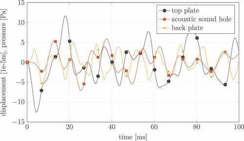
The time simulation of the FOM for an excitation frequency of $f=100\mathrm{H}\mathrm{z}$ is illustrated in Figure 6. The QoI displayed in the following figure are the excitation node on the top plate, the averaged pressure close to the sound hole and a structure node on the back plate. The quantities are calculated as

Figure 6. Time simulation of the QoI (20) with an excitation frequency $f=100\mathrm{H}\mathrm{z}$.

(20) $y_{\mathrm{Q}\mathrm{o}\mathrm{I},k}(t)={\mathit{c}}_{\mathrm{Q}\mathrm{o}\mathrm{I},k}^{\mathrm{\top }}\mathit{x}(t)\mathrm{w}\mathrm{i}\mathrm{t}\mathrm{h}k\in \left\{\mathrm{T}\mathrm{o}\mathrm{p}\mathrm{P}\mathrm{l}\mathrm{a}\mathrm{t}\mathrm{e},\mathrm{S}\mathrm{o}\mathrm{u}\mathrm{n}\mathrm{d}\mathrm{H}\mathrm{o}\mathrm{l}\mathrm{e},\mathrm{B}\mathrm{a}\mathrm{c}\mathrm{k}\mathrm{P}\mathrm{l}\mathrm{a}\mathrm{t}\mathrm{e}\right\}$(20)

with appropriately chosen QoI output vectors ${\mathit{c}}_{\mathrm{Q}\mathrm{o}\mathrm{I},k}^{\mathrm{\top }}$ for each QoI.

It can be seen that as a result of the excitation, the top plate at the excitation node starts to vibrate at the same frequency since the guitar describes a linear time-invariant (LTI) system. Note that, the only connection of the top plate and the back plate is through the air, since the side walls are considered as a fully reflective Neumann boundary condition on the fluid domain. In the area of FSI, a strong coupling implies a two-sided influence, where the structure is able to excite the fluid but also the fluid is capable of exciting the structure. In Figure 6, one can see that the input force excitation leads to a vibration of the top plate which thereupon transfers the energy to the air and the air in turn causes the vibration of the back plate, satisfying the conditions for a strong coupling. This chronological sequence can be observed by looking at the delayed rises in the curves.

3.2. Reformulations of the pH-system

We derived our pH-FSI-system via a transformation of the second-order system and using the displacements, the integrated pressure and their derivatives as pH variables. In classical Hamiltonian systems, the variables are defined in terms of the canonical position and momentum coordinates to account for additional symmetries [2]. For this reason, a system in momentum formulation shall also be considered in the analysis. All of the following reformulations of the pH-system still satisfy the mandatory pH properties (pH1) to (pH3). The coordinate transformation

(21) ${\mathit{x}}_m=\mathit{E}\mathit{x}$(21)

yields such a pH-system in momentum formulation (abbr.: Mom)³

(22) $\begin{array}{cc}{\dot{\mathit{x}}}_m& =(\mathit{J}-\mathit{D})\mathit{Q}{\mathit{E}}^{-1}{\mathit{x}}_m+\mathit{B}\mathit{u},\\ \mathit{y}& ={\mathit{B}}^{\mathrm{\top }}\mathit{Q}{\mathit{E}}^{-1}{\mathit{x}}_m,\end{array}$(22)

where ${\mathit{x}}_m$ contains the momentum instead of the velocities.

Since the PSD methods presented in Section 5.6 and 5.7 are based on a system formulation with canonical ${\mathbb{J}}_{2\hat{N}}$, i.e.

${\mathbb{J}}_{2\hat{N}}:=\left[\begin{array}{cc}\mathbf{0}& {\mathit{I}}_{\hat{N}}\\ -{\mathit{I}}_{\hat{N}}& \mathbf{0}\end{array}\right],$

the canonical variants of the velocity formulation

(23) ${\mathit{x}}_c={\mathit{P}}^{-1}\mathit{x}$(23)

and momentum formulation

(24) ${\mathit{x}}_{mc}={\mathit{P}}^{-1}\mathit{E}\mathit{x}$(24)

will be considered in the sensitivity analysis, which yields the canonical system in velocity formulation (abbr.: Vel_Canon)

(25) $\begin{array}{cc}{\mathit{P}}^{\mathrm{\top }}\mathit{E}\mathit{P}{\dot{\mathit{x}}}_c& ={\mathit{P}}^{\mathrm{\top }}(\mathit{J}-\mathit{D})\mathit{P}{\mathit{P}}^{-1}\mathit{Q}\mathit{P}{\mathit{x}}_c+{\mathit{P}}^{\mathrm{\top }}\mathit{B}\mathit{u},\\ \mathit{y}& ={\mathit{B}}^{\mathrm{\top }}\mathit{Q}\mathit{P}{\mathit{x}}_c\end{array}$(25)

and in momentum formulation (abbr.: Mom_Canon)

(26) $\begin{array}{cc}{\mathit{P}}^{\mathrm{\top }}\mathit{P}{\dot{\mathit{x}}}_{mc}& ={\mathit{P}}^{\mathrm{\top }}(\mathit{J}-\mathit{D})\mathit{P}{\mathit{P}}^{-1}\mathit{Q}{\mathit{E}}^{-1}\mathit{P}{\mathit{x}}_{mc}+{\mathit{P}}^{\mathrm{\top }}\mathit{B}\mathit{u},\\ \mathit{y}& ={\mathit{B}}^{\mathrm{\top }}\mathit{Q}{\mathit{E}}^{-1}\mathit{P}{\mathit{x}}_{mc}.\end{array}$(26)

The transformation matrices $\mathit{P},{\mathit{P}}^{-1}$ depend on the coupling matrix $\mathit{R}$ and are given by

(27) $\mathit{P}=\left[\begin{array}{cccc}{\mathit{I}}_{N_S}& \mathbf{0}& \mathbf{0}& -\mathit{R}/2\\ \mathbf{0}& {\mathit{I}}_{N_F}& {\mathit{R}}^{\mathrm{\top }}/2& \mathbf{0}\\ \mathbf{0}& \mathbf{0}& {\mathit{I}}_{N_S}& \mathbf{0}\\ \mathbf{0}& \mathbf{0}& \mathbf{0}& {\mathit{I}}_{N_F}\end{array}\right],\hspace{0.17em}{\mathit{P}}^{-1}=\left[\begin{array}{cccc}{\mathit{I}}_{N_S}& \mathbf{0}& \mathbf{0}& \mathit{R}/2\\ \mathbf{0}& {\mathit{I}}_{N_F}& -{\mathit{R}}^{\mathrm{\top }}/2& \mathbf{0}\\ \mathbf{0}& \mathbf{0}& {\mathit{I}}_{N_S}& \mathbf{0}\\ \mathbf{0}& \mathbf{0}& \mathbf{0}& {\mathit{I}}_{N_F}\end{array}\right].$(27)

The calculation of the FOM is computationally expensive, especially if it comes to multi-query simulations or the simulation of a more detailed guitar model with many more degrees of freedom. Therefore, MOR techniques are beneficial and will be discussed in the following.

4. Model order reduction – projection methods

The size of a dynamical system model can be reduced by approximating its behaviour in a subspace of a lower dimension. In most cases, this model reduction comes at the cost of approximation errors. Projection-based reduction methods can be performed in various ways with different outcomes with respect to the preservation of different structural⁴ pH properties, cf. ⑩.

All reduction methods used in our study are based on a projection-based reduction. The solution for $\mathit{x}(t)$ is approximated in a subspace $\mathcal{V}$ of dimension $n\ll N=2\hat{N}=2(N_S+N_F)$ which is described by a basis matrix $\mathit{V}\in {\mathbb{R}}^{N\times n}$ with $\mathrm{c}\mathrm{o}\mathrm{l}\mathrm{s}\mathrm{p}(\mathit{V})=\mathcal{V}$ and leads to the approximation

(28) $\mathit{x}(t)\approx \mathit{V}{\mathit{x}}_r(t)$(28)

with the reduced state vector ${\mathit{x}}_r\in {\mathbb{R}}^n$.

Inserting (28) into the pH-system (17) and using the Petrov-Galerkin condition for $\mathit{W}\in {\mathbb{R}}^{N\times n}$ [18] yields the reduced system

(29) $\begin{array}{cc}{\mathit{W}}^{\mathrm{\top }}\mathit{E}\mathit{V}{\dot{\mathit{x}}}_r& ={\mathit{W}}^{\mathrm{\top }}(\mathit{J}-\mathit{D})\mathit{Q}\mathit{V}{\mathit{x}}_r+{\mathit{W}}^{\mathrm{\top }}\mathit{B}\mathit{u}\\ \mathit{y}& ={\mathit{B}}^{\mathrm{\top }}\mathit{Q}\mathit{V}{\mathit{x}}_r.\end{array}$(29)

of size $n\ll N$, where the matrix $\mathit{W}$ determines the orthogonal projection direction.

4.1. Galerkin projection

A special case of the Petrov-Galerkin approach is given by the Galerkin projection (abbr.: Galerkin) with $\mathit{W}=\mathit{V}$ and takes the form

(30) $\begin{array}{cc}{\mathit{V}}^{\mathrm{\top }}\mathit{E}\mathit{V}{\dot{\mathit{x}}}_r& ={\mathit{V}}^{\mathrm{\top }}(\mathit{J}-\mathit{D})\mathit{Q}\mathit{V}{\mathit{x}}_r+{\mathit{V}}^{\mathrm{\top }}\mathit{B}\mathit{u}\\ \mathit{y}& ={\mathit{B}}^{\mathrm{\top }}\mathit{Q}\mathit{V}{\mathit{x}}_r.\end{array}$(30)

This projection does in general not preserve any of the underlying pH structure properties (pH1)–(pH3) of the system in our formulation.

4.2. Quasi-Galerkin projection

The quasi-Galerkin (abbr.: Quasi) projection is derived by inserting the term $\mathit{V}{\mathit{V}}^{\mathrm{\top }}$ under the assumption that $(\mathit{J}-\mathit{D})\mathit{V}{\mathit{V}}^{\mathrm{\top }}\mathit{Q}\approx (\mathit{J}-\mathit{D})\mathit{Q}$ to the standard Galerkin projection which yields

(31) $\begin{array}{cc}\underset{{\mathit{E}}_r}{\underbrace{{\mathit{V}}^{\mathrm{\top }}\mathit{E}\mathit{V}}}{\dot{\mathit{x}}}_r& ={\mathit{V}}^{\mathrm{\top }}(\mathit{J}-\mathit{D})\mathit{V}\underset{{\mathit{Q}}_r}{\underbrace{{\mathit{V}}^{\mathrm{\top }}\mathit{Q}\mathit{V}}}{\mathit{x}}_r+{\mathit{V}}^{\mathrm{\top }}\mathit{B}\mathit{u}\\ \mathit{y}& ={\mathit{B}}^{\mathrm{\top }}\mathit{Q}\mathit{V}{\mathit{x}}_r.\end{array}$(31)

This projection preserves (pH1) and (pH2) but it does not guarantee (pH3) and, hence, the Hamiltonian of the reduced system $\bar{\mathcal{H}}({\mathit{x}}_r)\ne \mathcal{H}(\mathit{V}{\mathit{x}}_r)$ changes in the reduction.

4.3. pH structure-preserving projection

Adapting the pH structure-preserving (abbr.: pH) approach [19] with $\mathit{W}=\mathit{Q}\mathit{V}$ to the case of a descriptor system leads to a reduced system

(32) $\begin{array}{cc}{\mathit{V}}^{\mathrm{\top }}{\mathit{Q}}^{\mathrm{\top }}\mathit{E}\mathit{V}{\dot{\mathit{x}}}_r& ={\mathit{V}}^{\mathrm{\top }}{\mathit{Q}}^{\mathrm{\top }}(\mathit{J}-\mathit{D})\mathit{Q}\mathit{V}{\mathit{x}}_r+{\mathit{V}}^{\mathrm{\top }}{\mathit{Q}}^{\mathrm{\top }}\mathit{B}\mathit{u}\\ \mathit{y}& ={\mathit{B}}^{\mathrm{\top }}\mathit{Q}\mathit{V}{\mathit{x}}_r\end{array}$(32)

with the reduced matrices

(33) $\begin{array}{cccc}{\mathit{E}}_r& ={\mathit{V}}^{\mathrm{\top }}{\mathit{Q}}^{\mathrm{\top }}\mathit{E}\mathit{V},& {\mathit{J}}_r& ={\mathit{V}}^{\mathrm{\top }}{\mathit{Q}}^{\mathrm{\top }}\mathit{J}\mathit{Q}\mathit{V},\\ {\mathit{D}}_r& ={\mathit{V}}^{\mathrm{\top }}{\mathit{Q}}^{\mathrm{\top }}\mathit{D}\mathit{Q}\mathit{V},& {\mathit{Q}}_r& ={\mathit{I}}_n.\end{array}$(33)

This preserves the pH properties (pH1)-(pH3) and does not change the Hamiltonian in the reduced system [19].

4.4. Energy-stable projection

The author in [20] presents a general framework for the numerical approximation of evolution problems which is also suitable for pH-systems and preserves the underlying Hamiltonian structure. We will call this approach energy-stable (abbr.: Energy-Stable). Applying this approach to a pH-system leads to a reduced system

(34) $\begin{array}{cc}{\mathit{V}}^{\mathrm{\top }}{\mathit{E}}^{\mathrm{\top }}{(\mathit{J}-\mathit{D})}^{-1}\mathit{E}\mathit{V}{\dot{\mathit{x}}}_r& ={\mathit{V}}^{\mathrm{\top }}{\mathit{E}}^{\mathrm{\top }}\mathit{Q}\mathit{V}{\mathit{x}}_r+{\mathit{V}}^{\mathrm{\top }}{\mathit{E}}^{\mathrm{\top }}{(\mathit{J}-\mathit{D})}^{-1}\mathit{B}\mathit{u},\\ \mathit{y}& ={\mathit{B}}^{\mathrm{\top }}\mathit{Q}\mathit{V}{\mathit{x}}_r.\end{array}$(34)

In our case, the inverse term can be easily calculated with

(35) $(\mathit{J}-\mathit{D}{)}^{-1}={\mathit{T}}^{\mathrm{\top }}{\mathit{P}}^{\mathrm{\top }}(\mathit{J}-\mathit{D})\mathit{P}\mathit{T}\mathrm{w}\mathrm{i}\mathrm{t}\mathrm{h}\mathit{T}=\left[\begin{array}{cc}\mathbf{0}& {\mathit{I}}_{\hat{N}}\\ {\mathit{I}}_{\hat{N}}& \mathbf{0}\end{array}\right]$(35)

which allows for a computational efficient implementation. To summarize the projection methods with emphasis on the structure-preservation properties, we enlist them in Table 2.

Table 2. Comparison of presented projection methods with the focus on structure-preservation.

Projection method	Feature	pH1	pH2	pH3
Galerkin	$\mathit{W}=\mathit{V}$	✘	✘	✘
Quasi	insert ${\mathit{V}}^{\mathrm{\top }}\mathit{V}$	✓	✓	✘
pH	$\mathit{W}=\mathit{Q}\mathit{V}$	✓	✓	✓
Energy-Stable	$\mathit{W}={\mathit{E}}^{\mathrm{\top }}(\mathit{J}-\mathit{D}{)}^{-\mathrm{\top }}\mathit{E}\mathit{V}$	✓	✓	✓

4.5. Best approximation

In order to assess the quality of the different projection methods, a direct comparison with the best approximation (abbr.: Bestapprox) in the considered subspace $\mathrm{c}\mathrm{o}\mathrm{l}\mathrm{s}\mathrm{p}(\mathit{V})$ should be examined. Here, we use the best approximation with respect to the energy norm $\parallel \cdot {\parallel }_{\mathcal{H}}^2$ induced by the energy inner product $⟨\cdot ,\cdot {⟩}_{\mathcal{H}}$

(36) $\parallel \mathit{x}{\parallel }_{\mathcal{H}}^2:={\mathit{x}}^{\mathrm{\top }}\mathit{H}\mathit{x}={\mathit{x}}^{\mathrm{\top }}{\mathit{E}}^{\mathrm{\top }}\mathit{Q}\mathit{x}=⟨\mathit{x},\mathit{x}{⟩}_{\mathcal{H}},$(36)

where $\mathit{H}={\mathit{E}}^{\mathrm{\top }}\mathit{Q}$ denotes the so-called energy matrix which is positive definite, since both ${\mathit{E}}^{\mathrm{\top }}$ and $\mathit{Q}$ are positive definite and their product is symmetric due to the third pH-property (pH3). The best approximation of $\mathit{x}$ in the subspace $\mathrm{c}\mathrm{o}\mathrm{l}\mathrm{s}\mathrm{p}(\mathit{V})$ is then given by the projection ${\mathrm{\Pi }}_{\mathit{V},\mathcal{H}}$ of $\mathit{x}$ onto $\mathrm{c}\mathrm{o}\mathrm{l}\mathrm{s}\mathrm{p}(\mathit{V})$ with respect to the energy inner product. In terms of the energy matrix, this can be expressed via

(37) ${\mathrm{\Pi }}_{\mathit{V},\mathcal{H}}\mathit{x}=\mathit{V}{\left({\mathit{V}}^{\mathrm{\top }}\mathit{H}\mathit{V}\right)}^{-1}{\mathit{V}}^{\mathrm{\top }}\mathit{H}\mathit{x}$(37)

and we have

(38) $\parallel \mathit{x}-{\mathrm{\Pi }}_{\mathit{V},\mathcal{H}}\mathit{x}{\parallel }_{\mathcal{H}}=\underset{\hat{\mathit{x}}\in \mathrm{c}\mathrm{o}\mathrm{l}\mathrm{s}\mathrm{p}(\mathit{V})}{min}\parallel \mathit{x}-\hat{\mathit{x}}{\parallel }_{\mathcal{H}}.$(38)

5. Model order reduction – basis generation

For all projection-based reduction methods presented in Section 4, a basis matrix $\mathit{V}$ is required. In the following, different basis generation approaches are presented with the goal to keep the approximation error as small as possible. The bases are generated by using the extensive software packages MatMorembs⁵ [47] and RBmatlab⁶, cf. ⑧ and ⑨.

5.1. Modal truncation

For the basis generation method based upon modal truncation (abbr.: Modal), the homogeneous solution for (17) with $\mathit{u}(t)=\mathbf{0}$ is solved with the ansatz function

(39) $\mathit{x}(t)=e^{{\lambda }_{j}t}{\varphi }_j\mathrm{w}\mathrm{i}\mathrm{t}\mathrm{h}{\lambda }_{\mathit{j}}\in \mathbb{C},{\varphi }_i,\in {\mathbb{C}}^N$(39)

which leads to the generalized eigenvalue problem

(40) $\mathit{A}{\varphi }_j={\lambda }_j\mathit{E}{\varphi }_j$(40)

with $\mathit{A}:=(\mathit{J}-\mathit{D})\mathit{Q}$ for the pH-system. The eigenvectors ${\varphi }_j$ are also called coupled eigenmodes and describe the deformation of the mechanical structure and pressure distribution in the fluid at the dedicated eigenfrequencies. Modal truncation uses only the most important eigenvectors as the projection basis [18]. In the context of the guitar, the most important eigenvectors coincide with the eigenvectors that belong to the lowest eigenfrequencies since those are assumed to be the crucial eigenfrequencies for the sound emission. Hence, the modal projection basis arises as

(41) ${\mathit{V}}_{mod}=\left[\begin{array}{ccc}{\varphi }_1& \dots & {\varphi }_n\end{array}\right]$(41)

with $n\ll N$. In the current study, the eigenmodes belonging to the lowest eigenfrequencies are coupled eigenmodes that allow for dynamics in the mechanical structure and fluid simultaneously. In general, ${\mathit{V}}_{mod}$ is not real-valued. In this case, the matrix ${\mathit{V}}_{mod}^{\mathrm{\top }}$ has to be replaced with ${\mathit{V}}_{mod}^H$ for the projection methods outlined in Section 4, where the superscript $\mathrm{H}$ represents the conjugate transpose of a complex-valued matrix.

5.2. Krylov-based reduction

The goal of Krylov-based reduction (abbr.: Krylov) is the approximation of the transfer function

(42) $\mathit{G}(s)={\mathit{B}}^{\mathrm{\top }}\mathit{Q}(s\mathit{E}-(\mathit{J}-\mathit{D})\mathit{Q}{)}^{-1}\mathit{B}$(42)

obtained from the Laplace transformation with the complex variable $s\in \mathbb{C}$ which is typically evaluated on the imaginary axis $s=i\omega$ with the circular frequency $\omega =2\pi f$ where $f$ denotes the excitation frequency.

The transfer function around an expansion point $s_0$ can be described with a Taylor series whose coefficients are called moments in this context. The first $J_b$ moments of the full and reduced system can be matched by using the block Krylov subspace of a pH-system

(43) $\text{colsp}(V_{Kry})={\mathcal{K}}_{J_b}({(A-s_{0}E)}^{-1}E,{(A-s_{0}E)}^{-1}B).$(43)

The approach can be generalized to calculate for multiple expansion points [18,22].

The direct calculation leads to numerical issues since additional vectors can become linearly dependent. That is why the block Arnoldi algorithm is used for the calculation of Krylov subspaces. This Arnoldi algorithm consists of a LU decomposition, Gram–Schmidt orthogonalization and the iterative calculation of Krylov directions [18,22]. Sometimes the approach is also called tangential interpolation [48].

5.3. POD full state

The Proper Orthogonal Decomposition (POD) approach uses a different idea for the projection basis generation, which is based on snapshots instead of system matrices and can therefore even be used for nonlinear systems [23,49]. The POD starts with a set of vectors ${\hat{\mathit{x}}}_k\in {\mathbb{R}}^N$ with $k=1,\dots ,m$ assembled column-wise into a matrix

(44) $\hat{\mathit{X}}:=\left[\begin{array}{ccc}{\hat{\mathit{x}}}_1& \dots & {\hat{\mathit{x}}}_m\end{array}\right].$(44)

The goal is to approximate the information contained in the snapshot matrix $\hat{\mathit{X}}$ by a set of vectors ${\hat{\mathit{u}}}_{\mathbf{j}}\in {\mathbb{R}}^N$ with $j=1,\dots ,n$, which can be expressed in terms of an optimization problem

(45) $\underset{{\hat{\mathit{u}}}_1,\dots ,{\hat{\mathit{u}}}_n}{min}\sum _{k=1}^m{∥{\hat{\mathit{x}}}_k-\sum _{j=1}^n{⟨{\hat{\mathit{x}}}_k,{\hat{\mathit{u}}}_j⟩}_{\mathcal{H}}{\hat{\mathit{u}}}_j∥}_{\mathcal{H}}^2\mathrm{s}\mathrm{u}\mathrm{b}\mathrm{j}\mathrm{e}\mathrm{c}\mathrm{t}\mathrm{t}\mathrm{o}⟨{\hat{\mathit{u}}}_k,{\hat{\mathit{u}}}_j{⟩}_{\mathcal{H}}={\delta }_{kj}$(45)

where ${\delta }_{kj}$ describes the Kronecker delta and, hence, the vectors ${\hat{\mathit{u}}}_j$ form an orthonormal basis with respect to the energy inner product [23]. The optimization problem can be solved as follows: we first solve the eigenvalue problem

(46) $H\widehat{X}{\widehat{X}}^T{\widehat{w}}_j={\lambda }_j{\widehat{w}}_j$(46)

with the scaled and weighted correlation matrix $H\widehat{X}{\widehat{X}}^T\in {ℝ}^{N\times N}$, then we solve the linear system

(47) $\mathit{H}{\hat{\mathit{v}}}_j={\hat{\mathit{w}}}_j$(47)

and finally, by normalizing the above with respect to the energy norm, i.e.

(48) ${\hat{\mathit{u}}}_j=\frac{1}{\parallel {\hat{\mathit{v}}}_j{\parallel }_{\mathcal{H}}}{\hat{\mathit{v}}}_j.$(48)

By only taking the first $n$ POD-modes, the basis matrix can be formed as

(49) ${\mathit{V}}_{\mathrm{P}\mathrm{O}\mathrm{D}}(\mathit{H},\hat{\mathit{X}}):=\left[\begin{array}{ccc}{\hat{\mathit{u}}}_1& \dots & {\hat{\mathit{u}}}_n\end{array}\right].$(49)

In the present system, the snapshot matrix $\hat{\mathit{X}}$ consists of state variables of the pH-system $\mathit{x}(t,\mu )$ with $\mu \in [82,320]\mathrm{H}\mathrm{z}$. The discrete trajectories that form the snapshot matrix are calculated from the full system with time instances of $\mathrm{\Delta }t={10}^{-4}\mathrm{s}$ for a time span of $T=0.1\mathrm{s}$. Using the full state vector (abbr.: POD-State) $\mathit{x}={\left[\begin{array}{cccc}{\mathit{z}}^{\mathrm{\top }}& {\mathit{q}}^{\mathrm{\top }}& {\dot{\mathit{z}}}^{\mathrm{\top }}& {\dot{\mathit{q}}}^{\mathrm{\top }}\end{array}\right]}^{\mathrm{\top }}$ for calculating, the POD basis will further be called as ${\mathit{V}}_{\mathrm{P}\mathrm{O}\mathrm{D},\mathrm{S}\mathrm{t}\mathrm{a}\mathrm{t}\mathrm{e}}$. Please note that while the above was introduced for the energy inner product, other inner products can also be considered simply by replacing the energy matrix $\mathit{H}$.

5.4. POD displacements

Another basis will be generated by only using the displacements (abbr.: POD-Disp) in the snapshot matrix ${\hat{\mathit{X}}}_{\mathrm{D}\mathrm{i}\mathrm{s}\mathrm{p}}=\left[\begin{array}{ccc}{\hat{\mathit{x}}}_{\mathrm{D}\mathrm{i}\mathrm{s}\mathrm{p},1}& \dots & {\hat{\mathit{x}}}_{\mathrm{D}\mathrm{i}\mathrm{s}\mathrm{p},m}\end{array}\right]$ of the adapted state vector ${\hat{\mathit{x}}}_{\mathrm{D}\mathrm{i}\mathrm{s}\mathrm{p},k}=\left[\begin{array}{cc}{\mathit{z}}_k^{\mathrm{\top }}& {\mathit{q}}_k^{\mathrm{\top }}\end{array}\right]$ and the inner product matrix $\mathit{K}$, which reflects the parts of the energy inner product stemming from only the displacements. We then assemble the full projection matrix afterwards as

(50) ${\mathit{V}}_{\mathrm{P}\mathrm{O}\mathrm{D}-\mathrm{D}\mathrm{i}\mathrm{s}\mathrm{p}}(\mathit{K},{\hat{\mathit{X}}}_{\mathrm{D}\mathrm{i}\mathrm{s}\mathrm{p}})=\left[\begin{array}{cc}{\mathit{V}}_{\mathrm{P}\mathrm{O}\mathrm{D}}(\mathit{K},{\hat{\mathit{X}}}_{\mathrm{D}\mathrm{i}\mathrm{s}\mathrm{p}})& \mathbf{0}\\ \mathbf{0}& {\mathit{V}}_{\mathrm{P}\mathrm{O}\mathrm{D}}(\mathit{K},{\hat{\mathit{X}}}_{\mathrm{D}\mathrm{i}\mathrm{s}\mathrm{p}})\end{array}\right].$(50)

Note that the above is a special case of the so-called tangent lift as presented in [24], where in (50) only information in the upper half of the state $\mathit{x}$ is considered. Hence, using the basis for the velocity component, i.e. lower half of the state $\mathit{x}$, might be ill-suited.

5.5. POD-Individual trajectories

A further approach will be the division of the state vector into the four individual parts and calculating the POD-basis for each individual trajectory (abbr.: POD-Indiv) and assembling the basis as the block-diagonal matrix

(51) $\begin{array}{rl}& {\mathit{V}}_{\mathrm{P}\mathrm{O}\mathrm{D}-\mathrm{I}\mathrm{n}\mathrm{d}\mathrm{i}\mathrm{v}}=\mathrm{b}\mathrm{l}\mathrm{k}\mathrm{d}\mathrm{i}\mathrm{a}\mathrm{g}\left({\mathit{V}}_{\mathrm{P}\mathrm{O}\mathrm{D}}({\mathit{K}}_S,{\hat{\mathit{X}}}_{\mathit{z}}),{\mathit{V}}_{\mathrm{P}\mathrm{O}\mathrm{D}}({\mathit{K}}_F/{\rho }_F,{\hat{\mathit{X}}}_{\mathit{q}}),\right.\\ & \left.{\mathit{V}}_{\mathrm{P}\mathrm{O}\mathrm{D}}({\mathit{M}}_S^{-1},{\hat{\mathit{X}}}_{\dot{\mathit{z}}}),{\mathit{V}}_{\mathrm{P}\mathrm{O}\mathrm{D}}({\rho }_F\cdot {\mathit{M}}_F^{-1},{\hat{\mathit{X}}}_{\dot{\mathit{q}}})\right)\end{array}$(51)

with the snapshot matrices ${\hat{\mathit{X}}}_{\mathit{z}}$, ${\hat{\mathit{X}}}_{\mathit{q}}$, ${\hat{\mathit{X}}}_{\dot{\mathit{z}}}$ and ${\hat{\mathit{X}}}_{\dot{\mathit{q}}}$ corresponding to the respective components of the state $\mathit{x}$ and the inner product matrices corresponding to the individual contribution to the energy inner product.

5.6. PSD Complex SVD

Symplectic MOR is structure-preserving MOR for Hamiltonian systems. One approach to derive a symplectic reduced-order basis is the data-driven Proper Symplectic Decomposition (PSD) which is closely related to the POD [24].

Assuming a suitable basis, a symplectic form ${\omega }_{2\hat{n}}:{\mathbb{R}}^{2\hat{n}}\times {\mathbb{R}}^{2\hat{n}}\to \mathbb{R}$ takes the canonical form

(52) ${\omega }_{2\hat{n}}({\mathit{v}}_1,{\mathit{v}}_2)={\mathit{v}}_1^{\mathrm{\top }}{\mathbb{J}}_{2\hat{n}}{\mathit{v}}_2\mathrm{\forall }{\mathit{v}}_1,{\mathit{v}}_2\in \mathbb{V}\mathrm{w}\mathrm{i}\mathrm{t}\mathrm{h}{\mathbb{J}}_{2\hat{n}}:=\left[\begin{array}{cc}{\mathbf{0}}_{\hat{n}}& {\mathit{I}}_{\hat{n}}\\ -{\mathit{I}}_{\hat{n}}& {\mathbf{0}}_{\hat{n}}\end{array}\right]$(52)

where ${\mathbb{J}}_{2\hat{n}}$ is the Poisson matrix with the identity matrix ${\mathit{I}}_{\hat{n}}\in {\mathbb{R}}^{\hat{n}\times \hat{n}}$ and the matrix of all zeros ${\mathbf{0}}_{\hat{n}}\in {\mathbb{R}}^{\hat{n}\times \hat{n}}$ [50]. We call $\mathit{V}\in {\mathbb{R}}^{2\hat{N}\times 2\hat{n}}$ a symplectic matrix if

(53) ${\mathit{V}}^{\mathrm{\top }}{\mathbb{J}}_{2\hat{N}}\mathit{V}={\mathbb{J}}_{2\hat{n}}.$(53)

If a Petrov-Galerkin projection is used with ${\mathit{W}}^{\mathrm{\top }}={\mathit{V}}^{+}$ where

(54) ${\mathit{V}}^{+}={\mathbb{J}}_{2\hat{n}}^{\mathrm{\top }}{\mathit{V}}^{\mathrm{\top }}{\mathbb{J}}_{2\hat{N}}\in {\mathbb{R}}^{2\hat{n}\times 2\hat{N}}$(54)

denotes the so-called symplectic inverse,⁷ then the Hamiltonian structure and therefore its Hamiltonian is preserved for purely Hamiltonian systems, i.e. in the case of $\mathit{D}=0$ in equation (14)(14) $\dot{x}\left(t\right)=(J-D)\nabla \mathscr{H}(x(t))+Bu\left(t\right)y\left(t\right)=B^T\nabla \mathscr{H}(x(t))$(14) [24, 25].

In analogy to the POD, the minimization problem appears as

(55) $\begin{array}{cc}\underset{\mathbf{V}\in {\mathbb{R}}^{2\hat{N}\times 2\hat{n}}}{\mathrm{m}\mathrm{i}\mathrm{n}\mathrm{i}\mathrm{m}\mathrm{i}\mathrm{z}\mathrm{e}}& \parallel ({\mathit{I}}_{2\hat{N}}-\mathit{V}{\mathit{V}}^{+})\hat{\mathit{X}}{\parallel }_F^2\\ \mathrm{s}\mathrm{u}\mathrm{b}\mathrm{j}\mathrm{e}\mathrm{c}\mathrm{t}\mathrm{t}\mathrm{o}& {\mathit{V}}^{\mathrm{\top }}{\mathbb{J}}_{2\hat{N}}\mathit{V}={\mathbb{J}}_{2\hat{n}},\end{array}$(55)

where the constraint guarantees that the reduced-order basis (ROB) is symplectic [24]. In contrast to POD, there is no explicit solution procedure for the PSD optimization problem (55). The PSD Complex SVD (abbr.: C-SVD) approach is the solution of the PSD in the subset of symplectic, orthonormal ROBs [25]. It uses an adapted complex snapshot matrix

(56) $C_s=\backslash \text{widetilde}{x}_1^s+i{\dot{\tilde{x}}}_1^s\dots {\tilde{x}}_m^s+i{\dot{\tilde{x}}}_m^s\in \widehat{N}\times \widehat{n}{x}_j^s=\left[z_j{q}_j\right]1\le j\le m$(56)

with the imaginary unit $i$. The minimization problem requires an auxiliary complex matrix ${\mathit{U}}_{{\mathit{C}}_s}\in {\mathbb{C}}^{\hat{N}\times \hat{n}}$ and takes the form

(57) $\begin{array}{cc}\underset{{\mathit{U}}_{{\mathit{C}}_s}\in {\mathbb{C}}^{2\hat{N}\times 2\hat{n}}}{\mathrm{m}\mathrm{i}\mathrm{n}\mathrm{i}\mathrm{m}\mathrm{i}\mathrm{z}\mathrm{e}}& \parallel {\mathit{C}}_s-{\mathit{U}}_{{\mathit{C}}_s}{({\mathit{U}}_{{\mathit{C}}_s})}^{\mathrm{H}}{\mathit{C}}_s{\parallel }_F^2\\ \mathrm{s}\mathrm{u}\mathrm{b}\mathrm{j}\mathrm{e}\mathrm{c}\mathrm{t}\mathrm{t}\mathrm{o}& {({\mathit{U}}_{{\mathit{C}}_s})}^{\mathrm{H}}{\mathit{U}}_{{\mathit{C}}_s}={\mathit{I}}_{\hat{n}}\end{array}$(57)

and generates the real basis matrix

(58) ${\mathit{V}}_{\mathrm{C}\mathrm{S}\mathrm{V}\mathrm{D}}:=\left[\begin{array}{cc}\tilde{\mathit{E}}& {\mathbb{J}}_{2\hat{N}}\tilde{\mathit{E}}\end{array}\right],\tilde{\mathit{E}}:=\left[\begin{array}{c}\mathrm{R}\mathrm{e}({\mathit{U}}_{{\mathit{C}}_s})\\ \mathrm{I}\mathrm{m}({\mathit{U}}_{{\mathit{C}}_s})\end{array}\right].$(58)

The speciality of the PSD Complex SVD is the choice of the auxiliary complex matrix ${\mathit{C}}_s$ and the computation of $\tilde{\mathit{E}}$ from ${\mathit{U}}_{{\mathit{C}}_s}$. The solution of (57) is the POD for complex matrices based on the left-singular vectors of ${\mathit{C}}_s$ that can be computed with a complex version of the SVD [24].

5.7. PSD SVD-like decomposition

Most existing basis generation techniques, e.g. Complex SVD, generate a symplectic, orthonormal ROB. In [25], a new symplectic, non-orthogonal basis generation technique based on the so-called SVD-like decomposition (abbr.: SVD-like) is introduced.

There exists an SVD-like decomposition of the snapshot matrix $\hat{\mathit{X}}\in {\mathbb{R}}^{2\hat{N}\times m}$

(59) $\begin{array}{rl}& \begin{array}{cccc}p& q& p& m-2p-q\end{array}\\ & \hat{\mathit{X}}={\mathit{S}}_s{\mathit{D}}_s{\mathit{Q}}_s,{\mathit{D}}_s=\left[\begin{array}{ccccccc}{\mathbf{\Sigma }}_s& \mathbf{0}& \mathbf{0}& \mathbf{0}& & & \\ \mathbf{0}& \mathit{I}& \mathbf{0}& \mathbf{0}\\ \mathbf{0}& \mathbf{0}& \mathbf{0}& \mathbf{0}\\ \mathbf{0}& \mathbf{0}& {\mathbf{\Sigma }}_s& \mathbf{0}\\ \mathbf{0}& \mathbf{0}& \mathbf{0}& \mathbf{0}\\ \mathbf{0}& \mathbf{0}& \mathbf{0}& \mathbf{0}\end{array}\right]\begin{array}{c}p\\ q\\ \hat{N}-p-q\\ p\\ q\\ \hat{N}-p-q\end{array},{\mathbf{\Sigma }}_s=\mathrm{d}\mathrm{i}\mathrm{a}\mathrm{g}({\sigma }_1,\dots ,{\sigma }_p)\in {\mathbb{R}}^{p\times p}\end{array}$(59)

with a symplectic matrix ${\mathit{S}}_s\in {\mathbb{R}}^{2\hat{N}\times 2\hat{N}}$, a sparse and potentially non-diagonal⁸ matrix ${\mathit{D}}_s\in {\mathbb{R}}^{2\hat{N}\times m}$, an orthogonal matrix ${\mathit{Q}}_s\in {\mathbb{R}}^{m\times m}$ and the symplectic singular values ${\sigma }_j$. The rank of the snapshot matrix is $\mathrm{r}\mathrm{a}\mathrm{n}\mathrm{k}(\hat{\mathit{X}})=2p+q$.

The Frobenius norm of the snapshot matrix can be rewritten as

(60) $\parallel \hat{\mathit{X}}{\parallel }_F^2=\mathrm{T}\mathrm{r}(\hat{\mathit{X}}{\hat{\mathit{X}}}^{\mathrm{\top }})=\sum _{j=1}^{p+q}(w_j{)}^2,w_j=\left\{\begin{array}{cc}{\sigma }_j\sqrt{\parallel {\mathit{s}}_i{\parallel }_2^2+\parallel {\mathit{s}}_{\hat{N}+j}{\parallel }_2^2}& 1\le j\le p\\ \parallel {\mathit{s}}_i{\parallel }_2,& p+1\le j\le p+q\end{array}\right.$(60)

where ${\mathit{s}}_j$ is the $j$-th column of ${\mathit{S}}_s$ and $w_j$ is called the weighted symplectic singular value [25].

The goal is to choose the $k$ indices $j\in {\mathcal{I}}_{\mathrm{S}\mathrm{V}\mathrm{D}}=\left\{j_1,\dots ,j_k\right\}\subset \left\{1,\dots ,p+q\right\}$ which have large contributions $w_j$ to the Frobenius norm with

(61) ${\mathcal{I}}_{\mathrm{S}\mathrm{V}\mathrm{D}}=\underset{\begin{array}{c}\mathcal{I}\subset \left\{1,\dots ,p+q\right\}\\ \left|\mathcal{I}\right|=k\end{array}}{\mathrm{a}\mathrm{r}\mathrm{g}\mathrm{m}\mathrm{a}\mathrm{x}}\left(\sum _{j\in \mathcal{I}}{(w_j)}^2\right)$(61)

which yields a ROB ${\mathit{V}}_{\mathrm{S}\mathrm{V}\mathrm{D}}\in {\mathbb{R}}^{2\hat{N}\times 2k}$ with $k$ pairs of columns ${\mathit{s}}_j\in {\mathbb{R}}^{2\hat{N}}$ from ${\mathit{S}}_s$ leading to reduced model order of $2k=n$ and the basis matrix

(62) ${\mathit{V}}_{\mathrm{S}\mathrm{V}\mathrm{D}}=\left[\begin{array}{cccccc}{\mathit{s}}_{j_1}& \dots & {\mathit{s}}_{j_k}& {\mathit{s}}_{\hat{N}+j_1}& \dots & {\mathit{s}}_{\hat{N}+j_k}\end{array}\right].$(62)

The SVD-like decomposition can be constructed by computing an eigendecomposition of ${\hat{\mathit{X}}}^{\mathrm{\top }}\mathit{J}\hat{\mathit{X}}$, for which the imaginary and real part of eigenvectors corresponding to complex conjugate eigenvalues result in a pair of symplectic vectors. Alternatively, one can use the approach introduced in [51], which does not require the computation of the product ${\hat{\mathit{X}}}^{\mathrm{\top }}\mathit{J}\hat{\mathit{X}}$ and only works with the snapshot matrix $\hat{\mathit{X}}$. However, for our numerical investigations, we chose the former method, as the implementation is rather straightforward.

Remark 2. Please note, that both, the PSD Complex SVD and PSD SVD-like decomposition, are usually considered for Hamiltonian systems. The FSI problem considered in this paper does not fall under this classification, since we have a non-zero damping influence, i.e. $\mathit{D}\ne 0$ in the confines of equation (14)(14) $\dot{x}\left(t\right)=(J-D)\nabla \mathscr{H}(x(t))+Bu\left(t\right)y\left(t\right)=B^T\nabla \mathscr{H}(x(t))$(14) . However, it is interesting to see how these basis generation techniques perform in the presence of dissipation. The limit $\mathit{D}\to 0$ would give a Hamiltonian system.

6. Results

The previous sections featured several alternatives for model order reduction of a classical guitar FSI problem in a pH formulation. The different components that were considered are the four system formulations in Sec. 3.2, the four projection methods from Sec. 4 and the seven basis generation methods in Sec. 5, cf. Figure 2. These categories are extended by choosing the reduced system size $n$, studying 11 sizes between $n=12$ and $n=400$ and the number of trajectories in the snapshot matrix for the data-based methods, where 6 alternatives were investigated. All representatives of each category can be combined with all others, resulting in a number of about $4\cdot 4\cdot 7\cdot 11\cdot 6\approx 7000$ possible combinations. All of these combinations have been computed on a computer with the specification from Table 3 and can be accessed in the form of a parallel coordinate plot at https://doi.org/10.18419/darus-3248. We will give a focused view onto the most important outcomes in the following sensitivity analysis.

Table 3. Specifications of hardware and software.

Operating system	Linux Debian 10.13
Processor	16 x Intel(R) Xeon(R) CPU E5-2643 0 @ 3.30 GHz
Memory (RAM)	129GB DDR3
Matlab version	R2020b
MatMorembs version	current version (08/2022)
RBmatlab version	1.16.09

In order to compare the different methods for reducing the FOM to a reduced-order model (ROM), cf. ⑪, an error measure is needed. The energy norm of the Hamiltonian

(63) $\parallel \mathit{x}(t){\parallel }_{\mathcal{H}}^2=\mathit{x}(t{)}^{\mathrm{\top }}{\mathit{E}}^{\mathrm{\top }}\mathit{Q}x(t)$(63)

is used to describe the energy value of a trajectory at time step $t$. The error $\epsilon (t)=\parallel \mathit{x}(t)-\mathit{V}{x}_r(t){\parallel }_{\mathcal{H}}$ between the full and reduced model is measured in the energy norm. In order to obtain a scalar and relative measure, the norm is integrated over the simulation time interval $I_t=[0,t_{\mathrm{e}\mathrm{n}\mathrm{d}}]$ and related to the full model which yields

(64) ${\epsilon }_r=\frac{{\int }_0^{t_{\mathrm{e}\mathrm{n}\mathrm{d}}}\parallel \mathit{x}\left(t\right)-\mathit{V}{\mathit{x}}_r\left(t\right){\parallel }_{\mathcal{H}}dt}{{\int }_0^{t_{\mathrm{e}\mathrm{n}\mathrm{d}}}\parallel \mathit{x}\left(t\right){\parallel }_{\mathcal{H}}dt}$(64)

for the relative error measure. It is important to use the relative error which allows for a comparison between different system inputs. Five randomly chosen frequencies in the standard tuning range (13) and zero initial conditions were used as system parameters for all experiments that were carried out. The mean value of their relative error calculations is displayed in the subsequent results.

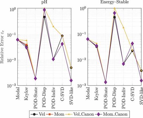
The relative error values for the four system formulations over all basis generation techniques and for the pH and energy-stable projections are illustrated in Figure 7. It can be seen that the displacement variant of POD is not a suitable option for all system reformulations. This is due to the fact that the state derivatives are not considered in the snapshot matrix, which are valuable information that should be contained. It does not lead to an improvement by focusing on the displacement and leaving the state trajectory independent from its derivatives. The canonical alternative for the velocity formulation (25) but also the non-canonical version (17) lead to higher errors for some basis generation techniques compared to the other reformulations. The momentum formulation for both, canonical (22) and non-canonical (26), leads to the best overall results, especially for POD-State and SVD-like. Since in the canonical transformation process, the block structure of the pH matrices $\mathit{E}$ and $\mathit{Q}$ (18) gets lost, we will focus on the non-canonical momentum formulation (22) in the remainder.

Figure 7. Relative error of different basis generation methods and system formulations for $n=120$.

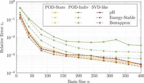
The three best-performing methods from the previous experiment, i.e. POD-State, SVD-like and POD-Individual, are compared more closely in Figure 8. The plot shows the development of the error of the three methods over the basis size and examines on the one hand the pH and energy-stable projections and on the other hand their behaviour in relation to the best approximation with respect to the energy norm, i.e. the FOM solution is projected onto the subspace spanned by the corresponding basis matrix respecting the inner product pertaining to the energy norm (38). One can see that the results of pH and energy-stable behave in a similar way for POD-State and SVD-like but for POD-Individual, the energy-stable projection leads to much better error values. The deviation concerning the best approximation does not exceed one order of magnitude for all basis generation methods, but again shows the largest margin for POD-Individual. POD-State remains the closest to its potential best values over the whole range of basis sizes. A comparison of the basis generation methods uncovers that the SVD-like and POD-State techniques lie in the range of the best approximation error of the POD-Individual method and show an improvement of approximately one order of magnitude for several reduction dimensions compared to the competitors. The overall behaviour of all basis generation techniques (even the one not shown in the plot) shows that the errors decay rapidly up to a size of $n=120$ and decrease more slowly starting from a size of approximately $n=200$. For this reason, further investigations are carried out for a basis size of $n=120$.

Figure 8. Relative error for three selected basis generation and projection methods in comparison with the best approximation.

The heat map in Figure 9 shows the relative error for all combinations of basis generation techniques and projection methods that were conducted, cf. ⑬. The errors are shown for a basis size of $n=120$. If the relative error exceeds a value of ${\epsilon }_r>1$, then the field entry is left blank.

Figure 9. Relative errors ${\epsilon }_r$ for different basis and projection combinations for $n=120$ in the momentum formulation.

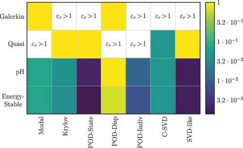
One can see that the Galerkin and Quasi-Galerkin projections perform the worst. These projections do not preserve the pH properties, especially the stability conditions, leading to instability and poor approximations. These projection methods are hence not suitable for the reduction of pH-systems. In general, the pH and energy-stable projection methods lead to the smallest error because of their adaption to the specific underlying pH structure of the system, which shows the importance of adapting the projection methods to the particular structure of the problem. The modal reduction, which is still used in various commercial MOR-packages, leads to high errors compared to the other combinations. The dynamics of the model cannot be described sufficiently accurate by only allowing to move in modal coordinates that belong to the lowest eigenfrequencies. A further comment on the modal reduction will be given in the output error discussion below. The basis generated with the C-SVD and Krylov algorithms leads to moderate approximation errors, which, in the case of the C-SVD, also cannot be improved by the transformation into the canonical structure of the matrix $\mathit{J}$. The Krylov algorithm focuses on approximating the input-output behaviour at certain frequencies, leading to higher error at different frequencies. The overall performance of the remaining data-based methods worked the best for the FSI dynamics of the guitar except for the POD-Displacement variant. The reason for the failure of the POD-Displacement has already been explained above. For the POD-State variant, the information contained in the snapshot matrix and extracted from this matrix via POD is sufficient for reproducing the coupled dynamics of the system. Both, the SVD-like and POD-State basis generation techniques, show the best overall performance with error values as low as ${\epsilon }_{r,\mathrm{S}\mathrm{V}\mathrm{D}-\mathrm{l}\mathrm{i}\mathrm{k}\mathrm{e}}=1.55\cdot {10}^{-3}$ and ${\epsilon }_{r,\mathrm{P}\mathrm{O}\mathrm{D}-\mathrm{S}\mathrm{t}\mathrm{a}\mathrm{t}\mathrm{e}}=1.88\cdot {10}^{-3}$. The explanation for this lies in the structure of the bases. The SVD-like approach is the only method that builds a non-orthogonal basis and can therefore adapt more flexibly to the system’s dynamics. Special attention should be paid here to the fact that the SVD-like method was developed for purely Hamiltonian systems, whereas this study shows that it is also suitable for port-Hamiltonian systems. The POD-State method is adapted to the problem in the sense that it uses the energy inner product induced by the Hamiltonian which significantly improves the reduction results compared to the standard inner product.

It is worth mentioning that the information content in the snapshot matrices depends on the number of underlying trajectories which are randomly distributed in the parameter space. In the following study, trajectory numbers between 5 and 100 are investigated. The results of the associated relative errors are shown in Table 4 and are extended by the methods based on system matrices for comparison. It can be seen that the influence of a high number of trajectories is not as significant as, for instance, the size of the reduced system, see Figure 8. All methods extract enough information for basis constructions even for small snapshot sizes. A snapshot matrix made of 10 trajectories already shows a good trade-off between approximation error and matrix size, which drastically decreases the computational effort in the offline phase due to few evaluations of the full system.

Table 4. Relative error of various basis generation methods over the number of trajectories from the snapshot generation for the momentum formulation, pH projection and $n=120$. One trajectory refers to an excitation with one specific frequency.

	Number of trajectories
Basis Generation	5	10	25	50	75	100
Modal	0.0635	no data-based method, ${\epsilon }_r$ for the sake of completeness
Krylov	0.0402	no data-based method, ${\epsilon }_r$ for the sake of completeness
POD-State	0.0022	0.0020	0.0018	0.0019	0.0019	0.0019
POD-Disp	0.9492	0.9497	0.9494	0.9496	0.9496	0.9496
POD-Indiv	0.0211	0.0219	0.0151	0.0119	0.0109	0.0108
C-SVD	0.1307	0.0993	0.0488	0.0465	0.0439	0.0432
SVD-like	0.0019	0.0018	0.0016	0.0016	0.0016	0.0016

The main goal of MOR is the gain of a speed-up compared to the simulation of the full-order model to make this model suitable for multi-query tasks or real-time scenarios. The speed-up values are determined for the pH projection method and averaged over all basis generation methods since the qualitative behaviour for the other methods was similar. The results for the velocity (17) and the momentum (22) formulations are listed in Table 5. The greatest speed-up of more than $1000$ in the case of the velocity formulation and $6000$ for the momentum formulation is obtained with a basis size of $n=12$. This choice is not recommendable, since the error values are very high for this size. The speed-up values decrease down to $69$ (Vel) and $313$ (Mom) for a basis size of $n=400$. Depending on the requirements for the ROM, one needs to decide which is the best trade-off between approximation quality and gained speed-up. Since the error decays fast up to a size of $n=120$ and still leads to speed-ups of more than $297$ (Vel) and $1610$ (Mom), this reduction size was focused on in the previous discussion.

Table 5. Averaged speed-up values for different basis sizes for the pH projection.

Basis size	12	40	80	120	200	280	400
Speed Up (Vel)	1093	811	528	297	120	104	69
Speed Up (Mom)	6342	3860	2821	1610	519	494	313

In (15), we stated that a pH-system satisfies the dissipation inequality, which leads to the useful properties of passivity and stability. The goal of structure-preserving model reduction and the time discretization with an IMR is the preservation of these properties. Hence, in Figure 10 the dissipation inequality is exemplified for all model order reduction techniques under a pH-structure-preserving projection (32). Therefore, the dissipation inequality (15) is converted to

Figure 10. Dissipation inequality bound for the pH-projection and a system in momentum formulation $n=120$.

(65) $\mathcal{H}(\mathit{x}(t_1))-\mathcal{H}(\mathit{x}(t_0))-{\int }_{t_0}^{t_1}\mathit{y}(t{)}^{\mathrm{\top }}\mathit{u}(t)dt\le 0\mathrm{w}\mathrm{i}\mathrm{t}\mathrm{h}{t}_1>t_0$(65)

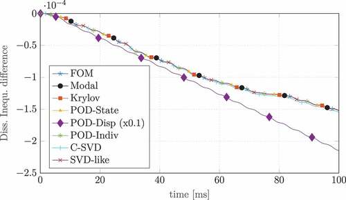
which gives us a bound of $0$ that is displayed in Figure 10. One can see that all trajectories satisfy the dissipation inequality over the whole time interval which agrees with the theory from the MOR and time integration. The decrease in the energy can be explained by the energy losses due to the structural dissipation effects. Note that the POD-Disp variant is scaled by a factor of $0.1$ due to higher error values in the trajectory and therefore a considerably different Hamiltonian.

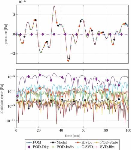
In Figure 11 and Figure 12, the QoI of the displacement of the excitation node on the top plate and the averaged pressure in the sound hole, cf. Figure 5, are depicted. Both figures contain two subfigures, where the first subfigure displays the time trajectory of the FOM and the corresponding ROM trajectories for all basis generation methods and the second subfigure illustrates the absolute error in the QoI, calculated as

Figure 11. Time simulation and absolute error $e_{\mathrm{Q}\mathrm{o}\mathrm{I},\mathrm{T}\mathrm{o}\mathrm{p}\mathrm{P}\mathrm{l}\mathrm{a}\mathrm{t}\mathrm{e}}$ of the excitation node displacement for the full and reduced-order models for $n=120$ and $f=200\mathrm{H}\mathrm{z}$ in the momentum formulation and pH projection.

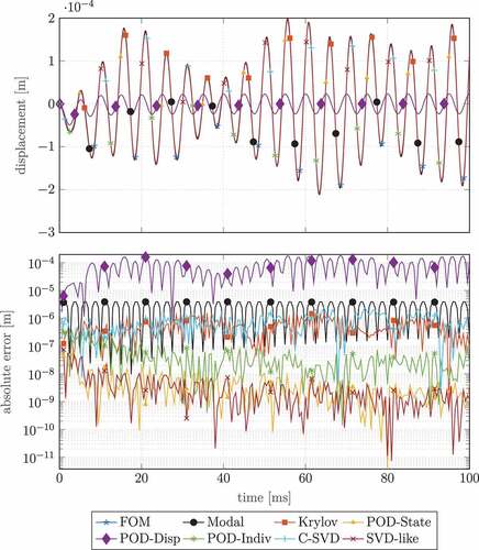
Figure 12. Time simulation and absolute error $e_{\mathrm{Q}\mathrm{o}\mathrm{I},\mathrm{S}\mathrm{o}\mathrm{u}\mathrm{n}\mathrm{d}\mathrm{H}\mathrm{o}\mathrm{l}\mathrm{e}}$ of the pressure integral over the sound hole for the full and reduced-order models for $n=120$ and $f=200\mathrm{H}\mathrm{z}$ in the momentum formulation and pH projection.

(66) $e_{\mathrm{Q}\mathrm{o}\mathrm{I},k}=y_{\mathrm{Q}\mathrm{o}\mathrm{I},k}-y_{r,\mathrm{Q}\mathrm{o}\mathrm{I},k}\mathrm{w}\mathrm{i}\mathrm{t}\mathrm{h}k\in \left\{\mathrm{T}\mathrm{o}\mathrm{p}\mathrm{P}\mathrm{l}\mathrm{a}\mathrm{t}\mathrm{e},\mathrm{S}\mathrm{o}\mathrm{u}\mathrm{n}\mathrm{d}\mathrm{H}\mathrm{o}\mathrm{l}\mathrm{e}\right\}$(66)

based on the QoI output (20) for the FOM and reduced model.

We can see in both cases that all basis construction methods except for POD-Displacement capture the behaviour quite well as the differences in the trajectories are almost not visible. For the POD-Displacement, however, almost no energy seems to be introduced into the system, which is unphysical, resulting in no visible excitation in the entire FSI model. The general behaviour of the previous error discussion can also be seen in the QoI absolute errors, namely that excellent performance of the POD-State and SVD-like approaches and the moderate performance of Krylov and C-SVD. Interestingly, the POD-Individual method performs better in the structural domain (see Figure 11) than in the fluid domain (see Figure 12), which shows that the underlying structural motions are better represented in the POD-modes. The converse can be seen for the modal approach. The eigenmodes that belong to the lowest eigenfrequencies approximate the fluid domain quite accurately, even in the same order of magnitude as the best MOR approaches, whereas the structural modes cannot be reproduced satisfactorily.

7. Conclusion and Outlook

In this paper, we presented a port-Hamiltonian formulation of a fluid–structure interaction for the case of a classical guitar. Many different model order reduction approaches combined with multiple different reduced basis construction methods as well as various FOM formulations were compared in order to study the effect of structure-preserving model reduction on the quality and behaviour of the reduced model. In particular, we were able to conclude that both structure-preserving model order reduction methods, i.e. the pH-preserving and the energy-stable methods clearly outperform their non-structure-preserving competitors. Furthermore, we can conclude that the reduced bases constructed via a symplectic SVD-like decomposition and a POD method that takes the energy inner product into account result in higher quality approximations for lower basis sizes.

Future emphasis will be placed on constructing suitable a-posteriori error estimators and extending the above model to allow for further parameter dependency in the form of material parameters of the guitar body.

Disclosure statement

No potential conflict of interest was reported by the author(s).

Correction Statement

This article has been republished with minor changes. These changes do not impact the academic content of the article.

Additional information

Funding

Supported by (DFG, German Research Foundation) Project Nos. 314733389, 455440338, and under Germany’s Excellence Strategy - Stuttgart Center for Simulation Science, Universität Stuttgart EXC 2075 – 390740016. We acknowledge the support by the Stuttgart Center for Simulation Science (SimTech; Deutsche Forschungsgemeinschaft).

Notes

1. Note that the term structure has an ambiguity in this paper. On the one hand, it describes the mechanical structure of the wooden guitar plates as part of the fluid–structure interaction. On the other hand, it likewise describes the mathematical structure of the pH-system, which should be preserved through the model reduction process. To avoid misunderstandings, the expression mechanical structure is used in the context of the FSI.

2. The theoretical background of the so-called length correction comes from the theory of the Helmholtz resonator, as one of the most basic resonant structures with a short tube and an acoustic cavity, see [52]. Here, the length correction of the tube is used to match resonant frequencies with measurement results and literature values, cf [53].

3. Labels are already introduced in the definition of various formulations, which are used for the later analysis of results in order to increase the readability of the outcomes

4. Here, the term structure refers to the mathematical pH structure.

5. www.itm.uni-stuttgart.de/software/morembs/software_morembs_matmorembs/

6. https://www.morepas.org/software/rbmatlab/

7. Please note that this symplectic inverse should not be confused with the Moore-Penrose inverse, which sometimes is denoted with the same symbol.

8. In general, the space spanned by the columns of $\hat{\mathit{X}}$ might not be spanned exclusively by pairs of symplectic vectors. In this case, using the notation in equation (59)(59) $\begin{array}{rl}& \begin{array}{cccc}p& q& p& m-2p-q\end{array}\\ & \hat{\mathit{X}}={\mathit{S}}_s{\mathit{D}}_s{\mathit{Q}}_s,{\mathit{D}}_s=\left[\begin{array}{ccccccc}{\mathbf{\Sigma }}_s& \mathbf{0}& \mathbf{0}& \mathbf{0}& & & \\ \mathbf{0}& \mathit{I}& \mathbf{0}& \mathbf{0}\\ \mathbf{0}& \mathbf{0}& \mathbf{0}& \mathbf{0}\\ \mathbf{0}& \mathbf{0}& {\mathbf{\Sigma }}_s& \mathbf{0}\\ \mathbf{0}& \mathbf{0}& \mathbf{0}& \mathbf{0}\\ \mathbf{0}& \mathbf{0}& \mathbf{0}& \mathbf{0}\end{array}\right]\begin{array}{c}p\\ q\\ \hat{N}-p-q\\ p\\ q\\ \hat{N}-p-q\end{array},{\mathbf{\Sigma }}_s=\mathrm{d}\mathrm{i}\mathrm{a}\mathrm{g}({\sigma }_1,\dots ,{\sigma }_p)\in {\mathbb{R}}^{p\times p}\end{array}$(59) , they have $\hat{N}\ne 2p$ and thus, we obtain a zero row in the block structure of ${\mathit{D}}_S$. For our numerical experiments, this case does not appear.

References

- A. van der Schaft and D. Jeltsema, Port-Hamiltonian systems theory: An introductory overview, Foundations and Trends in Systems and Control. 1 (2014), pp. 173–378. 10.1561/2600000002.
- S. Chaturantabut, C. Beattie, and S. Gugercin, Structure-preserving model reduction for nonlinear port-Hamiltonian systems, SIAM Journal on Scientific Computing. 38 (2016), pp. B837–B865. 10.1137/15M1055085.
- R. Rashad, F. Califano, A. Schaft, and S. Stramigioli, Twenty years of distributed port-Hamiltonian systems: A literature review, IMA Journal of Mathematical Control and Information. 37 (2020), pp. 1400–1422. 10.1093/imamci/dnaa018.
- H.J. Bungartz and M. Schäfer, Fluid-structure Interaction: Modelling, Simulation, Optimisation, Vol. 53, Berlin Heidelberg: Springer Science & Business Media, 2006.
- T. Richter, Fluid-structure Interactions: Models, Analysis and Finite Elements, Vol. 118, Cham: Springer, 2017.
- A. Brauchler, P. Ziegler, and P. Eberhard, An entirely reverse-engineered finite element model of a classical guitar in comparison with experimental data, The Journal of the Acoustical Society of America. 149 (2021), pp. 4450–4462. 10.1121/10.0005310.
- O. Christensen, Quantitative models for low frequency guitar function, Journal of Guitar Acoustics. 6 (1982), pp. 10–25. http://scholar.google.com/scholar_lookup?hl=en.
- E. Bécache, G. Derveaux, and P. Joly, An efficient numerical method for the resolution of the Kirchhoff-Love dynamic plate equation, Numerical Methods for Partial Differential Equations. 21 (2005), pp. 323–348. https://onlinelibrary.wiley.com/doi/abs/10.1002/num.20041.
- A. Brauchler, P. Ziegler, and P. Eberhard, Examination of polarization coupling in a plucked musical instrument string via experiments and simulations, Acta Acustica. 4 (2020), pp. 9. 10.1051/aacus/2020008. paper no. 9 (12 pages).
- M. Ducceschi and S. Bilbao, Linear stiff string vibrations in musical acoustics: Assessment and comparison of models, The Journal of the Acoustical Society of America. 140 (2016), pp. 2445–2454. 10.1121/1.4962553.
- G. Derveaux, A. Chaigne, P. Joly, and E. Bécache, Time-domain simulation of a guitar: Model and method, The Journal of the Acoustical Society of America. 114 (2003), pp. 3368–3383. 10.1121/1.1629302.
- E. Bécache, A. Chaigne, G. Derveaux, and P. Joly, Numerical simulation of a guitar, Computers & Structures. 83 (2005), pp. 107–126. 10.1016/j.compstruc.2004.04.018.
- F. Silva, T. Hélie, and V. Wetzel, Port-Hamiltonian Representation of Dynamical Systems. Application to Self-Sustained Oscillations in the Vocal Apparatus, in 7th Int. Conf. on Nonlinear Vibrations, Localization and Energy Transfer, P. du Lma, ed., Vol. 160, Jun, Marseille, France. 2019, Available at https://hal.archives-ouvertes.fr/hal-03020400.
- A. Falaize and T. Hélie, Passive simulation of the nonlinear port-Hamiltonian modeling of a Rhodes piano, Journal of Sound and Vibration. 390 (2017), pp.289–309. https://www.sciencedirect.com/science/article/pii/S0022460X16306320.
- M. Tchonkova and S. Sture, Classical and recent formulations for linear elasticity, Archives of Computational Methods in Engineering. 8 (2001), pp. 41–74. 10.1007/BF02736684.
- D. Blackstock, Fundamentals of Physical Acoustics, Wiley, New York, 2000.
- O.C. Zienkiewicz, R.L. Taylor, and D.D. Fox, The Finite Element Method for Solid and Structural Mechanics, 7th ed., Butterworth-Heinemann, Oxford, 2013.
- A. Antoulas, Approximation of Large-Scale Dynamical Systems, SIAM, Philadelphia, 2005.
- T. Wolf, B. Lohmann, R. Eid, and P. Kotyczka, Passivity and structure preserving order reduction of linear port-Hamiltonian systems using Krylov subspaces, European Journal of Control. 16 (2010), pp. 401–406. 10.3166/ejc.16.401-406.
- H. Egger, O. Habrich, and V. Shashkov, On the energy stable approximation of Hamiltonian and gradient systems, Computational Methods in Applied Mathematics. 21 (2021), pp. 335–349. 10.1515/cmam-2020-0025.
- P. Koutsovasilis and M. Beitelschmidt, Comparison of model reduction techniques for large mechanical systems, Multibody System Dynamics. 20 (2008), pp. 111–128. 10.1007/s11044-008-9116-4.
- R. Freund, Model reduction methods based on Krylov subspaces, Acta Numerica. 12 (2003), pp. 267–319. http://journals.cambridge.org/action/displayAbstract?fromPage=onlineaid=165629fulltextType=RAfileId=S0962492902000120.
- S. Volkwein, Proper orthogonal decomposition: Theory and reduced-order modelling, http://www.math.uni-konstanz.de/numerik/personen/volkwein/teaching/POD-Book.pdf (2013).
- L. Peng and K. Mohseni, Symplectic model reduction of Hamiltonian systems, SIAM Journal on Scientific Computing. 38 (2016), pp. A1–A27. 10.1137/140978922.
- P. Buchfink, A. Bhatt, and B. Haasdonk, Symplectic model order reduction with non-orthonormal bases, Mathematical and Computational Applications. 24 (2019), pp.43. https://www.mdpi.com/2297-8747/24/2/43.
- C. Beattie, S. Gugercin, and V. Mehrmann, Structure-preserving interpolatory model reduction for port-Hamiltonian differential-algebraic systems, in Realization and Model Reduction of Dynamical Systems: A Festschrift in Honor of the 70th Birthday of Thanos Antoulas, C. Beattie, P. Benner, M. Embree, S. Gugercin, and S. Lefteriu, eds., Structured Dynamical Systems, Springer International Publishing, Cham, 2022, pp. 235–254. 10.1007/978-3-030-95157-3_13.
- J.S. Hesthaven, C. Pagliantini, and N. Ripamonti, Structure-preserving model order reduction of Hamiltonian systems (2021). Available at https://arxiv.org/abs/2109.12367.
- R. Altmann, V. Mehrmann, and B. Unger, Port-Hamiltonian formulations of poroelastic network models, Mathematical and Computer Modelling of Dynamical Systems. 27 (2021), pp. 429–452. 10.1080/13873954.2021.1975137.
- J. Hesthaven and C. Pagliantini, Structure-preserving reduced basis methods for Poisson systems, Mathematics of Computation. 90 (2021), pp. 1701–1740. 10.1090/mcom/3618.
- O.C. Zienkiewicz, R.L. Taylor, and J.Z. Zhu, The Finite Element Method – Its Basis & Fundamentals, Butterworth-Heinemann, Oxford, 2005.
- A. Tkachuk and M. Bischoff, Variational methods for selective mass scaling, Computational Mechanics. 52 (2013), pp. 563–570. 10.1007/s00466-013-0832-0.
- A. Brauchler, D. Hose, P. Ziegler, M. Hanss, and P. Eberhard, Distinguishing geometrically identical instruments: Possibilistic identification of material parameters in a parametrically model order reduced finite element model of a classical guitar, Journal of Sound and Vibration. 535 (2022), pp.117071. https://www.sciencedirect.com/science/article/pii/S0022460X22002838.
- D. Matignon and T. Hélie, A class of damping models preserving eigenspaces for linear conservative port-Hamiltonian systems, European Journal of Control. 19 (2013), pp.486–494. https://www.sciencedirect.com/science/article/pii/S0947358013001672.
- R. Lerch, G. Sessler, and D. Wolf, Technische Akustik - Grundlagen und Anwendungen, Springer Berlin Heidelberg, Wiesbaden, 2009.
- C. Howard and B. Cazzolato, Acoustic Analyses Using Matlab and Ansys, Boca Raton, FL: Taylor & Francis Group, 2017.
- A. van de Walle, F. Naets, E. Deckers, and W. Desmet, Stability-preserving model order reduction for time-domain simulation of vibro-acoustic FE models, International Journal for Numerical Methods in Engineering. 109 (2017), pp. 889–912. https://onlinelibrary.wiley.com/doi/abs/10.1002/nme.5323.
- G. Everstine, A symmetric potential formulation for fluid-structure interaction, Journal of Sound and Vibration. 79 (1981), pp. 157–160. 10.1016/0022-460x(81).
- Abaqus, Abaqus Theory Manual, Providence, RI: Abaqus, Inc, 2016.
- V. Mehrmann and R. Morandin, Structure-preserving discretization for port-Hamiltonian descriptor systems, in 2019 IEEE 58th Conference on Decision and Control (CDC), Nice. 2019, pp. 6863–6868, Available at 10.1109/CDC40024.2019.9030180.
- C. Beattie, V. Mehrmann, H. Xu, and H. Zwart, Linear port-Hamiltonian descriptor systems, Mathematics of Control, Signals and Systems. 30 (2018). 10.1007/s00498-018-0223-3.
- A. Ezcurra, M. Elejabarrieta, and C. Santamaría, Fluid–structure coupling in the guitar box: Numerical and experimental comparative study, Applied Acoustics. 66 (2005), pp.411–425. https://www.sciencedirect.com/science/article/pii/S0003682X04001240.
- T. Breiten, R. Morandin, and P. Schulze, Error bounds for port-Hamiltonian model and controller reduction based on system balancing, Computers & Mathematics with Applications. 116 (2022), pp.100–115. https://www.sciencedirect.com/science/article/pii/S0898122121003102.
- F.L. Cardoso-Ribeiro, D. Matignon, and L. Lefèvre, A Partitioned Finite Element Method for power-preserving Discretization of Open Systems of Conservation Laws, IMA Journal of Mathematical Control and Information. 38 (2020), pp. 493–533. 10.1093/imamci/dnaa038.
- P. Kotyczka and L. Lefèvre, Discrete-time port-Hamiltonian systems: A definition based on symplectic integration, Systems & Control Letters. 133 (2019), pp.104530. https://www.sciencedirect.com/science/article/pii/S0167691119301409.
- E. Celledoni and E.H. Høiseth, Energy-preserving and passivity-consistent numerical discretization of port-Hamiltonian systems, arXiv: Numerical Analysis (2017). https://arxiv.org/abs/1706.08621.
- S. Aoues, D. Eberard, and W. Marquis-Favre, Canonical interconnection of discrete linear port-Hamiltonian systems, in 52nd IEEE Conference on Decision and Control, Firenze. 2013, pp. 3166–3171, 10.1109/CDC.2013.6760366.
- J. Fehr, D. Grunert, P. Holzwarth, B. Fröhlich, N. Walker, and P. Eberhard, Morembs—a model order reduction package for elastic multibody systems and beyond, in Reduced-Order Modeling (ROM) for Simulation and Optimization: Powerful Algorithms as Key Enablers for Scientific Computing, W. Keiper, A. Milde, and S. Volkwein, eds., Springer International Publishing, Cham, 2018, pp. 141–166. 10.1007/978-3-319-75319-5_7.
- A. Castagnotto, Optimal model reduction by tangential interpolation: H2 and Hinf perspectives, Dissertation, Technical University Munich, Munich (2018). http://mediatum.ub.tum.de/?id=1437106.
- R. Pinnau, Model order reduction: Theory, research aspects and applications, in Model Order Reduction: Theory, Research Aspects and Applications, in Model Reduction via Proper Orthogonal Decomposition, W.H.A. Schilders, H.A. van der Vorst, and J. Rommes, eds., 1st, Vol. 13 Springer Berlin Heidelberg, Berlin, Heidelberg, 2008, pp. 95–109. 10.1007/978-3-540-78841-6_5.
- A.C.D. Silva, Lectures on Symplectic Geometry, Springer, Berlin, Heidelberg, 2008.
- H. Xu, A numerical method for computing an SVD-like decomposition, SIAM J. Matrix Analysis Applications. 26 (2005), pp. 1058–1082. 10.1137/S0895479802410529.
- L. Li, Y. Liu, F. Zhang, and Z. Sun, Several explanations on the theoretical formula of Helmholtz resonator, Advances in Engineering Software. 114 (2017), pp.361–371. https://www.sciencedirect.com/science/article/pii/S096599781730635X.
- N. Fletcher and T. Rossing, The Physics of Musical Instruments, Springer Science & Business Media, New York, 1991.