Comparison of the strip- and block-wise aerial triangulation using different exterior orientation parameters weights

ABSTRACT

In this study, three different procedures: checkpoint RMS of residuals, statistical evaluation of AT results using t-test, and comparison of a photogrammetric digital surface model (DSM) and LiDAR data are used to analyse the effect of IMU and GNSS uncertainties on the final adjusted results. The outcome suggests that the method of block-wise GNSS shift correction is the better method for aerial triangulation and one should use appropriate observable weights in AT. The comparison of checkpoint RMS residuals between the two methods shows that the block-wise solution is on average 6cm more accurate than the strip-wise solution.

KEYWORDS:

• Direct georeferencing
• aerial triangulation
• mobile mapping
• GNSS/INS integration
• shift and drift effects

Introduction

Determining the Exterior Orientation Parameters (EOPs) (i.e. position and orientation of camera projection centre) is the most crucial task within the photogrammetric process. Nowadays, sensor orientation is possible in different ways. Aerial triangulation (AT) usually counts as a conventional model for 3D reconstruction problems or nonlinear least-squares problems utilizing image correspondences (Snavely et al. 2008), where the errors in observables based on probability theory have a normal distribution, i.e. Gaussian distribution (Triggs et al. 1999, Baselga 2007, Hohle 2008, Gerke 2009, Zach 2014).

Besides classical AT, which is the indirect technique for determining the EOPs using GCPs, Direct Georeferencing (DG) without the use of any GCPs or least GCPs is also possible with high-accuracy integrated GNSS and IMU (Cramer 1999, Lembicz 2006, Rizaldy and Firdaus 2012, Shi et al. 2017, El-Ashmawy 2018). However, the GCPs are necessary for quality assurance and control (Cramer 1999, Madani and Mostafa 2001). Cramer (2001) introduced a strip-wise integration approach for combining the imaging sensor and integrated data of continuously recorded GPS and INS data in a Kalman filter approach. He showed that the final accuracy of the DG without using GCPs was about 8–11 and 15–23 μm in image space for the horizontal and vertical components, respectively. In other words, with medium-scale flight, i.e. an altitude of about 2000 m, the object points are determined to an accuracy of 10–20 cm for the horizontal and 20–30 cm for the vertical coordinates. DG has three prominent benefits rather than applying classical AT, i.e. shorter time for data processing, mild workflow and lower cost project at the same accuracy (Pfeifer et al. 2012). A variety of observables and constraints with different scales and dimensions can play a prominent role in AT calculation. They are included as image points, Ground Control Points (GCPs), EOPs (i.e. global navigation satellite systems (GNSS) and inertial measurement unit (IMU) observables) (Lembicz 2006, Ip et al. 2007), right angles (Gerke 2011) and parallel lines (Zhang et al. 2011) are used. The proper way of handling the observables or constraints in an AT is to weigh their contributions by appropriately assigning a priori uncertainties. For instance, automatic tie-points extraction uncertainty is between 0.1 and 0.5 pixels (Gruen 2012) and automatic tie-point generation performance is improved using proper GNSS/INS data (Kiraci and Toz 2016). On the other hand, manual tie-points extraction uncertainty is presumed to have 0.5 pixels. This means that for GCPs the uncertainty can be from 0.05 m to 0.5 m using GNSS or other surveying techniques (Yuan et al. 2009, Gülch 2012). However, spatial distribution and lower precision of the tie-points influence the reliable estimation of the EOPs of the camera centre (Truong Giang et al. 2018). The automatic AT accuracy still depends on the forward and lateral overlap, distribution of GCPs and the accuracy of EOPs for use in the AT process. Some researchers have shown that automatic AT has some restrictions for extracting tie-points in some areas such as lakes, forests and mountain areas (Kersten et al. 1998, Heipke 1999, Seifert et al. 2019) and the challenging scenarios occur when there are few small matchable objects in images (Kerner et al. 2016). Due to the aforementioned restrictions, it is inevitable for the collection of GNSS/IMU data during photogrammetry projects for easing the photogrammetric process. On-board GNSS/IMU uncertainties would be divided into positioning and attitude uncertainties where positioning uncertainty varies between 0.05~0.3 m. in principle .005 ~ .008 degree for the attitude uncertainty is definitely under the good survey condition (Ip et al. 2007, Xie et al. 2016). Hence, assigning the optimum observable uncertainties (i.e. GNSS and IMU) is an important step in AT, which is the focus of this study.

The GNSS shift and drift effects in AT are the other indispensable issue that taken into consideration in this research. Accurate stereo plotting and orthophoto production are not reachable by directly recorded GNSS/IMU EOPs due to some errors such as shift and drift systematic errors of GNSS, atmospheric effects, camera calibration and accuracy, and coordinate system handling (Heipke et al. 2002). GNSS shift and drift correction besides the IMU-to-camera boresight misalignment angle could significantly change the result in Bundle Block Adjustment (BBA) (Madani and Shkolnikov 2005, Yastikli et al. 2007, Blázquez and Colomina 2012). These two would be vanished from the functional models using relative aerial control instead of absolute position and attitude for each image. Combined GPS/block adjustment is the other topic that some researchers worked on it, for example, Schmitz et al. (2001), introduced the rigorous GPS modelling in the combined GPS/block adjustment. They showed that this approach has some advantages relative to the shift and drift corrections. It was suggested the IMU besides GPS-supported AT provides better final accuracy.

IMU comprises three accelerometers and three gyroscopes. The accelerometers, in addition to measuring gravitational acceleration in triad orthogonal directions, also measure noise. Therefore, accelerometer observables are reliable only in long-term measurements and require a low pass filter for removing noise. However, the gyroscope calculates the orientation angles in triad orthogonal directions by integrating the angular rate in unit time. Accordingly, integrating in unit time causes cumulative errors; thus, the gyroscope’s observables are only reliable in the short term (Jouybari et al. 2019). The roll, pitch and yaw angles are used for transforming a vector from the body coordinate into an image coordinate system and vice versa. The position and orientation (roll, pitch and yaw) of a moving platform accurately can be attained using different types of filtering (Jouybari et al. 2017).

Several research groups have studied the effect of observable errors in AT. Mostafa et al. (2001a) present an error analysis for the airborne DG technique where EOPs are directly obtained using POS/Av 510 airborne positioning and attitude determination system. They investigated the DG accuracy in conjunction with the standard stereo model and a single image. The results showed that the accuracy of DG meets the theoretical admissible accuracy for map production. Moreover, Mostafa and Hutton (2001b) compared an independent photogrammetrically derived reference trajectory with the US National Geodetic Survey (NGS) Continuously Operating Reference Stations (CORS) as a base station of airborne GPS survey in individual and combined configurations. The result proves that CORS can be used as base stations in the USA mobile mapping industry, specifically, if the station distribution is dense and data acquisition frequency is high. Kruck (2001) used two different GNSS/IMU sensors, from Applanix and IGI companies, and compared the performance of the sensors using two different image scales, i.e. 1:5000 and 1:1000. GNSS/IMU sensor from Applanix had a lower Root Mean Square (RMS) rather than the IGI even though the number of GNSS satellites (in the DG) in the two scenarios were different.

In this paper, we use a dataset (manned aerial photogrammetry) over the Gothenburg region to investigate the effect of different observable uncertainties, i.e. GNSS and IMU measurements, in the block adjustment calculation. The GNSS shift and drift effects are modelled by constant (shift) and linear (drift) components in strip-wise and block-wise scenarios. The results are evaluated by examining the checkpoint RMS of residuals and using a statistical t-test for determining the number of images with gross error and finally, photogrammetric DSM is compared with DTM generated by Lidar point cloud.

Study area and data

A test area was selected to analyse the strip-wise and block-wise GNSS shift and drift corrections. The data were collected on 8 July 2018, over the Gothenburg test area, in the southwest part of Sweden. Lantmäteriet, the Swedish mapping, cadastral and land registration authority, collected the data, in the form of a photogrammetry block of a large area with 0.25 m Ground Sample Distance (GSD). The aircraft was flown with 3700-m altitude and 60% and 25% forward and lateral overlap. The test field area is approximately 75 × 90 km² with 24 strips, 1198 images, 18 full control points, 28 vertical control points, 10 horizontal and 19 vertical checkpoints. The horizontal components ($E,N$) of GCPs measured on top of the house roofs with the Real-Time Kinematic method for each point. However, the vertical component (H) was calculated with interpolating of well-situated points, e.g. on asphalt or road using a national height model obtained from aerial laser scanning results (Lantmateriet 2020) with the point density of at least 0.5 points/m². The mean distance between laser points is at most approx. 1.4 m. GCPs and checkpoint coordinates are measured in SWEREF 99 and RH2000 reference system and estimated positional accuracies are ${\hspace{0.17em}}_{-}^{+}3cm$ for Horizontal and ${\hspace{0.17em}}_{-}^{+}5cm$ for the vertical component. Figure 1 shows the camera’s perspective centre and distribution of all GCPs and checkpoints’ locations in the test field which is overlaid on a land cover of the region. Copernicus (Copernicus Europe’s eyes on Earth, 2020) which was initiated in 1985 provided the CORINE Land Cover (CLC) inventory, but the latest update which we used is CLC2018. The CLC2018 data were gathered by Sentinel-2 (Geometric accuracy ≤10 m) and the gaps were filled with Landsat-8 data.

Figure 1. Left: land cover of the test field with images perspective centres, ground control points and check point’s location. Right: the location of the photogrammetric block (black configuration) in Sweden.

The GNSS/IMU equipment, POS AV 510, supported by Applanix industry expertise and technological innovation was used in this project (Figure S1). This system integrates a dual-frequency GNSS receiver using differential carrier phase measurements and high-quality IMU. Lantmäteriet used an UltraCam Eagle digital camera with an 80 mm lens. The specifications of the camera and POS AV show that the positional accuracy is between 0.05 and 0.3 m roll and pitch better than 0.005$\text{^^circ}$and yaw better than 0.008$\text{^^circ}$(Table S1).

Theoretical background

In what follows, the mathematical model of the AT and the effects of different factors such as the GNSS shift and drift effects in the AT are explained.

Aerial triangulation (Bundle Block Adjustment)

A 3D position of the object on the ground employing the aerial image is attainable using the orientation parameters and position of an aerial image. The classical mathematical model of the BBA, which is used to compute the object, coordinates by aerial image coordinates is based on the collinearity equation. The collinearity equation is a physical model based on the geometry of a bundle of rays that represents the connection between image points, object points on the ground and the projection centre of the camera sensor (Osada 2001, Kraus 2007, Blázquez and Colomina 2012, Wierzbicki 2017):

(1) $f_x^{\hspace{0.17em}}=\left({x{ }^{\mathrm{\prime }}}_0+d_{{x{ }^{\mathrm{\prime }}}_0}\right)-\left(\mathrm{f}+d_{\mathrm{f}}\right)\times \left[\frac{r_{11}\left(X-X_0\right)+r_{21}\left(Y-Y_0\right)+r_{31}\left(Z-Z_0\right)}{r_{13}\left(X-X_0\right)+r_{23}\left(Y-Y_0\right)+r_{33}\left(Z-Z_0\right)}\right]+{\delta }_{shift}+\left(t-t_0\right){\delta }_{drift}$(1)

(2) $f_y^{\hspace{0.17em}}=\left({y{ }^{\mathrm{\prime }}}_0+d_{{y{ }^{\mathrm{\prime }}}_0}\right)-\left(\mathrm{f}+d_{\mathrm{f}}\right)\times \left[\frac{r_{12}\left(X-X_0\right)+r_{22}\left(Y-Y_0\right)+r_{32}\left(Z-Z_0\right)}{r_{13}\left(X-X_0\right)+r_{23}\left(Y-Y_0\right)+r_{33}\left(Z-Z_0\right)}\right]+{\delta }_{shift}+\left(t-t_0\right){\delta }_{drift}$(2)

where $x{{ }^{\mathrm{\prime }}}_0,y{{ }^{\mathrm{\prime }}}_0$ are the image coordinate of the principal point and ${\mathrm{d}}_{{\mathrm{x}{ }^{\mathrm{\prime }}}_0},{\mathrm{d}}_{{\mathrm{y}{ }^{\mathrm{\prime }}}_0}$ are the correction of the coordinates of the principal point. $\mathrm{f}$ is calibrated focal length and $d_f$ is a correction of the focal length. $r_{ij}$ are the rotation matrix arrays of $R(\omega ,\phi ,\kappa )$ between the image coordinate system and the ground coordinate system, $X,Y,Z$ are object coordinates, $X_0,Y_0,Z_0$ are the position of projection centre in the ground coordinate system,${\delta }_{shift}={\left[\begin{array}{ccc}\delta x_{shift}& \delta y_{shift}& \delta z_{shift}\end{array}\right]}^T$ and ${\delta }_{drift}={\left[\begin{array}{ccc}\delta x_{drift}& \delta y_{drift}& \delta z_{drift}\end{array}\right]}^T$ are the shift/drift corrections in 3D, and $\left(t-t_0\right)$ depicts that drift is grown by time $\left(t\right)$ w.r.t. the reference time $\left(t_0\right)$. ${\delta }_{shift}$ and ${\delta }_{drift}$ will be discussed more in the next section.

After determining the unknown parameters (i.e. EOPs) using least-square adjustment, a statistical test should be performed. The most important test is evaluating the posterior variance factor that should be tested using a t-test (Bjerhammar 1973). The assumed a priori variance factor and the estimated one should be the same and equal, otherwise, the used weights can be too optimistic or pessimistic. Therefore, the weights should be changed and repeat the adjustment process. The observable weights should be analysed after the BBA because the observables that are measured during aerial photogrammetry are noisy and consequently one should assign the optimum weights.

A t-test can be also used for evaluation of the AT quality by finding the number of gross errors due to assigning optimistic or pessimistic observable weights. The t-test examines two estimates that are from the same component. The two estimates typically represent two different times (e.g., pre-processing and post-processing variables). Generally, a t-test can be written as follows:

(3) $t_{obs}=\left|\frac{\hat{L}\mathbf{-}L}{u(\hat{L}-L)}\right|\le t_{n-1,\alpha /2}$(3)

and

(4) $u(\hat{L}\mathbf{-}L)=\sqrt{u^2(\hat{L})+u^2(L)}$(4)

where $\hat{L}$ is the EOPs after the AT and $L$ is the EOPs before the AT. Also, $u(\hat{L})$ and $u(L)$ are $\hat{L}$ and $L$ uncertainties, respectively. It is assumed that the EOPs are measured an infinite number of times and one can assess that if any of the observables are not acceptable at $\alpha =5\mathrm{\%}$significance level (risk level) with $n-1$ degrees of freedom. Thus, if$\left|t_{obs}\right|>1.96$, there would be a gross error due to assigning unrealistic weights for EOPs after the AT.

GNSS shift and drift correction

It is important to take the GNSS shift and drift effects into consideration in the extended mathematical model of AT (Tsai et al. 2006, Wierzbicki 2017). The use of shift and drift corrections in AT process (see Equations 1(1) $f_x^{\hspace{0.17em}}=\left({x{ }^{\mathrm{\prime }}}_0+d_{{x{ }^{\mathrm{\prime }}}_0}\right)-\left(\mathrm{f}+d_{\mathrm{f}}\right)\times \left[\frac{r_{11}\left(X-X_0\right)+r_{21}\left(Y-Y_0\right)+r_{31}\left(Z-Z_0\right)}{r_{13}\left(X-X_0\right)+r_{23}\left(Y-Y_0\right)+r_{33}\left(Z-Z_0\right)}\right]+{\delta }_{shift}+\left(t-t_0\right){\delta }_{drift}$(1) and 2(2) $f_y^{\hspace{0.17em}}=\left({y{ }^{\mathrm{\prime }}}_0+d_{{y{ }^{\mathrm{\prime }}}_0}\right)-\left(\mathrm{f}+d_{\mathrm{f}}\right)\times \left[\frac{r_{12}\left(X-X_0\right)+r_{22}\left(Y-Y_0\right)+r_{32}\left(Z-Z_0\right)}{r_{13}\left(X-X_0\right)+r_{23}\left(Y-Y_0\right)+r_{33}\left(Z-Z_0\right)}\right]+{\delta }_{shift}+\left(t-t_0\right){\delta }_{drift}$(2) ) principally impacts on precision and accuracy of determination of EOPs and the distribution of the residuals for the GNSS observations (Schmitz et al. 2001, Mesas-Carrascosa et al. 2014). The GNSS shift and drift corrections are classified into two parts, i.e. a systematic shift and a linear drift (increase by time) (Figure 2). The constant shift forms the major portion of the GNSS shift and drifts the correction domain; thus, in some cases, correcting just the systematic shift is satisfactory (Wierzbicki 2017).

Figure 2. Systematic shift and linear drift errors, modified after Trimble (2015).

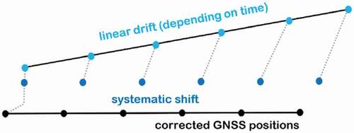
The shift and drift correction in Trimble Inpho Match-AT software is computed in two methods (i.e. block-wise and optionally strip-wise). The strip-wise approach is a method that calculates the synchronization offset between the GNSS receiver and camera sensor in each strip as well as other strip-wise effects. Linear drift and constant shift coefficients are two sets of correction coefficients, which are computed by the strip-wise method, but the block-wise method just determines the shift coefficient and it needs a proper distribution of GCPs in the project area. Block-wise GNSS shift corrections are used for correcting the GNSS observables, due to unsolved datum corrections between the GNSS and GCP coordinate system. The block-wise shift correction method needs the GCPs in the corner of the block when a high-accuracy GNSS measurement is given.

Data processing

The effect of different GNSS and IMU observable uncertainties on the final accuracy of the block adjustment is assessed in this study. This assessment is carried out in two strip-wise and block-wise scenarios. In the strip-wise scenario, the effect of GNSS and IMU observable uncertainties is investigated strip by strip for calculating the GNSS shift and drift corrections, whereas GNSS shift and drift corrections in the block-wise approach are accomplished for the whole block at the same time. Trimble Inpho Match-AT software, version 8.0.9.55161 is used for data processing. Land cover is important in the tie-point extraction stage, e.g. fewer tie-points are normally extracted in the forest and water land area rather than built-up area due to more detectable objects on the ground (Kersten et al. 1998, Heipke 1999, Kerner et al. 2016, Seifert et al. 2019). Therefore, firstly, tie-point is extracted automatically by software then after a quality check by the Photogrammetry operator some of them were removed and some added manually.

To evaluate the results and compare them, firstly, the checkpoint RMS of residuals is evaluated in the strip- and block-wise approaches for various a priori observable uncertainties (GNSS and IMU data). The a priori uncertainties that are considered for the IMU observables varied between 0.001 and 0.009$\text{^^circ}$with a 0.001$\text{^^circ}$interval for each step, and for the GNSS observables varied between 0.04 and 0.36 m with 0.04 m increments for each step. Two different scenarios are considered in this study: (1) different IMU observable uncertainties and assuming a constant GNSS observable uncertainty, i.e. 0.2, 0.2 and 0.2 m for $E,N,H$ coordinates, respectively, and (2) different GNSS observable uncertainties and assuming a constant IMU observable uncertainty i.e. 0.003$\text{^^circ}$, 0.003$\text{^^circ}$and 0.007$\text{^^circ}$ for $\omega ,\phi ,\kappa$, respectively. We have also considered the proposed Lantmäteriet default GNSS and IMU uncertainties, i.e. 0.2 m for $E,N,H$ coordinates and 0.003$\text{^^circ}$, 0.003$\text{^^circ}$ and 0.007$\text{^^circ}$ for $\omega ,\phi ,\kappa$, respectively, which were used as reference values to see how different uncertainties influence the RMS of residuals of the checkpoints.

In such two scenarios, some a priori uncertainty is set for other constraints in AT calculation. These include 0.1 m for the GCPs (for the horizontal components), 0.25 m for GCPs (for the vertical component), 0.004 mm for the automatic, and 0.002 mm for the manual measurements of image points. Secondly, the numbers of rejected images were calculated using a statistical hypothesis test, i.e., t-test (using Equation 3)(3) $t_{obs}=\left|\frac{\hat{L}\mathbf{-}L}{u(\hat{L}-L)}\right|\le t_{n-1,\alpha /2}$(3) . In this step, the captured data will be assessed by evaluating the quality of the calculated EOPs and the RMS residual of checkpoints. Finally, LiDAR DTM and photogrammetric DSM are analysed to confirm which uncertainty is working better in a flat area, i.e. a road.

Results and discussion

Checkpoint RMS of residuals

The checkpoint RMS of residuals, in height component, is calculated for the strip-wise and block-wise approaches. The vertical checkpoints are taken for the survey because the horizontal checkpoints only cover the bare-land and built-up areas but not forest and green-land areas. Tables S2 and S3 show the results of the first scenario by considering a priori observable uncertainties of IMU data between 0.001~ 0.009$\text{^^circ}$ and the uncertainties of GNSS data are assumed to be constant, i.e. 0.2, 0.2 and 0.2 m for $E,N,H$coordinates, respectively. In the second scenario, a -priori observable uncertainties of GNSS data varied between 0.04 and 0.36 m, and the constant values of 0.003$\text{^^circ}$, 0.003$\text{^^circ}$ and 0.007$\text{^^circ}$ for $\omega ,\phi ,\kappa$, respectively, were assigned for IMU data (Tables S4 and S5). According to Table S2, the best checkpoint RMS of residuals in the strip-wise method is 0.196 m, which is 0.065 m better than the residuals obtained using the Lantmäteriet default values. Besides, in Table S3 the best RMS of residuals in the block-wise method is 0.151 m, which is 0.017 m better than the Lantmäteriet default values. Considering everything, the results show that the block-wise method has better performance when one uses different IMU uncertainties (i.e. 0.008$\text{^^circ}$for $\omega ,\phi$ and 0.002$\text{^^circ}$ for$\kappa$) and constant 0.2 m for GNSS uncertainties.

Forasmuch as the vertical coordinate derived from GNSS positioning is intrinsically less accurate than the horizontal coordinates, it is expected that vertical accuracy to be ordinarily about 1.5 to 3 times worse than the horizontal accuracy (Cramer et al. 2000). The $\kappa$value should usually be less accurate than $\omega ,\phi$ that refers to the GNSS/IMU characteristics. $\kappa$ is from the yaw angle and this is always the critical angle for a GNSS/IMU solution (Scherzinger 1996). The a priori observable uncertainty of yaw for a POS/AV 510 unit is 0.008$\text{^^circ}$, while roll and pitch are 0.005$\text{^^circ}$. Consequently, the GNSS horizontal components and ($\omega ,\phi$) have been segregated from the vertical component and respectively, in this study. Therefore, it is expected $\kappa$should usually be less accurate than Comparison of GCPs’ vertical residual vectors for case 1 and 2. Again, the better performance of case 2 is shown. This scenario will be investigated, shown in Table S5, with further higher GNSS uncertainty and lower IMU uncertainty (e.g. 0.05 grads or 0.045 arc-degree) in the BBA. The influence of GNSS shift and drift effects in the AT was also studied by Kruck (2001). He showed that the IMU observable and uncertainties have no significant effect on the AT results. However, in contrast to the Kruck (2001) claims, we found that by changing the IMU uncertainty (i.e. 0.008 for $\omega ,\phi$, 0.002 for $\kappa$) one could obtain a better checkpoint RMS residual in the block adjustment. In this part, we have found a better uncertainty to reduce the effect of GNSS shift and drift corrections. Blázquez and Colomina (2012) proposed functional models that can completely remove the effect of GNSS shift and drift from the BBA process. They showed that the checkpoint RMS of residuals is approximately less than 0.06 m. This functional model needs further investigations in future studies.

By assuming different GNSS and constant IMU uncertainties, the best checkpoint RMS of residual in the strip-wise method is 0.239 m, which is 0.084 m better than using the Lantmäteriet default values (Table S4). Besides, Table S5 shows that the best checkpoint RMS of residuals in the block-wise method is 0.156 m, which is 0.012 m better than using the default values. Generally, based on these two tables (S4 and S5), the block-wise method shows better results for different GNSS and default IMU uncertainties.

Contrary to the findings of Pfeifer et al. (2012) who claimed that using the strip-wise linear modelling for the GPS shift and drift corrections was the better choice, we did not find the same result at least in drift values. In this regard, Block-wise and strip-wise drift value plotted (Figure S2.1) together with horizontal and vertical shift value (Figures S2.2 and S2.3) for specific uncertainty (i.e. 0.02 m for the GNSS and 0.003 °, 0.003 °, 0.007 ° for the IMU) to illustrate how each strip drift value can be different from the block-wise drift value. The strip-wise method calculates drift values separately for each strip and Figure S2.1 shows large drift values in the strips. However, drift values for Block-wise will be zero in three directions and similar results can be seen in Wierzbicki (2017). Our results show that using the block-wise method is the better approach for GNSS shift and drift corrections due to having zero drift values.

Evaluation of AT quality using t-test

Bypassing the first test, i.e. checking the RMS of residuals, the block-wise method is selected for the next step, i.e. assessing image gross errors using a t-test by comparing the EOPs before and after adjustment. Table 1 shows different observable uncertainty that is compared in terms of RMS residual checkpoints and the number of the rejected images using the statistical t-test.

Table 1. The number of rejected images and checkpoint RMS of some best case, worst case and Lantmäteriet default (*) values for observable uncertainties.

Observable uncertainty
GNSS (metre)	IMU ($\text{^^circ}$)	Numbers of rejected image							RMS Residual check Points (m)
u(E), u(N), u(H)	u(ω), u(φ), u($\kappa$)	E	N	H	ω	φ	$\mathit{\kappa }$	Total
0.2, 0.2, 0.2	0.007, 0.007, 0.009	0	1	0	0	0	0	1	0.157
	0.006, 0.006, 0.008	0	1	0	1	0	0	2	0.158
	0.008, 0.008, 0.002	0	1	0	0	0	537	538	0.151
	0.003, 0.003, 0.007	0	0	0	92	0	3	95	0.168	*
	0.001, 0.001, 0.001	36	33	0	1188	2	748	2007	0.184
	0.001, 0.001, 0.009	1	0	0	1193	1	0	1195	0.192
0.08, 0.08, 0.08	0.003, 0.003, 0.007	1	6	0	65	0	3	75	0.157
0.04, 0.04, 0.04		0	3	14	60	0	3	80	0.157
0.12, 0.12, 0.12		1	5	0	76	0	3	85	0.16
0.2, 0.2, 0.2		0	0	0	92	0	3	95	0.168	*
0.36, 0.36,0.2		0	0	0	100	0	3	103	0.177
0.36, 0.36, 0.36		0	0	0	102	0	3	105	0.181
0.08, 0.08, 0.08	0.007, 0.007, 0.009	0	7	1	0	0	0	8	0.154

Concerning Tables S3 and S4, all the possible observables uncertainties have been tested for the block-wise method using different IMU and constant GNSS observable uncertainties (i.e. 0.2 m for $E,N,H$). In this study, according to Table 1, assuming 0.2, 0.2 and 0.2 m for GNSS observable uncertainty and 0.007$\text{^^circ}$, 0.007$\text{^^circ}$ and 0.009$\text{^^circ}$for IMU observable uncertainty is the best case due to the least RMS residual of checkpoints and the minimum number of rejected images. The best-case shows there is only one rejected image (see Figure 3); however, the 0.02, 0.02 and 0.02 m for the GNSS observable uncertainty and 0.006$\text{^^circ}$, 0.006$\text{^^circ}$, 0.008$\text{^^circ}$ for the IMU observable uncertainty have approximately the same accuracy, i.e. with just two rejected images. 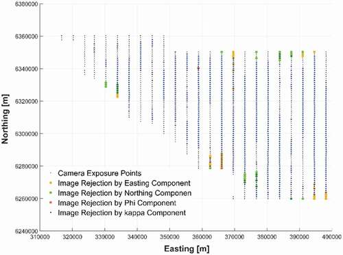By considering the GNSS observable uncertainty equal to 0.2, 0.2 and 0.2 m, and 0.001$\text{^^circ}$, 0.001$\text{^^circ}$ and 0.001$\text{^^circ}$for the IMU observable uncertainty, a large RMS of residuals (for the checkpoints) and the maximum number of images with gross error will be obtained that is the worst case in this study. In the worst case, 2007 rejected images are obtained according to Figure 4 (it should be noted the 2007 image is th summation of the rejected images for each of six EOPs elements, i.e. $E,N,H$, $\omega ,\phi$ and $\kappa$).

Figure 3. The minimum number of rejected images when using 0.007$\text{^^circ}$, 0.007$\text{^^circ}$ and 0.009$\text{^^circ}$uncertainties for $\omega ,\phi ,\kappa$ also 0.2 m uncertainties for $E,N,H$, respectively.

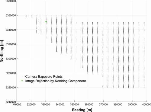
Figure 4. The maximum number of rejected images when using 0.001$\text{^^circ}$, 0.001$\text{^^circ}$ and 0.001$\text{^^circ}$uncertainties for $\omega ,\phi ,\kappa$ also 0.2 m uncertainties for $E,N,H$, respectively (all images rejected by $\omega$ but it is not shown in this figure).

All the possible observables uncertainty, obtained from Table S5, has been tested for the block-wise using different GNSS and constant IMU observable uncertainty (0.003$\text{^^circ}$for $\omega ,\phi$ and 0.007$\text{^^circ}$ for $\kappa$). According to Table 1, the rejected images in the best case (minimum number of images with gross error) with 75 images rejected and the worst case (maximum number of images with gross errors) with 105 rejected images are shown in Figures S3 and S4, respectively.

Options that are more reliable exist, for example, by employing the best IMU observable uncertainty, i.e. 0.007$\text{^^circ}$, 0.007$\text{^^circ}$, and 0.009$\text{^^circ}$while the GNSS observable uncertainty is constant (0.2 m). Also, using the best GNSS observable uncertainty, i.e. 0.08, 0.08 and 0.08 m while the IMU observable uncertainty is constant (i.e. 0.003$\text{^^circ}$, 0.003$\text{^^circ}$ and 0.007$\text{^^circ}$) one can obtain trustworthy results. In this case, the RMS residual checkpoints are 0.154 m (last row in Table 1) and the number of rejected images is just eight images (Figure S5). Three observable uncertainties have been selected using the first test (less RMS residual of checkpoints) and the second test (the minimum number of rejected images). The three best observable uncertainties are defined as follows in this study: [0.2 m for GNSS and 0.007$\text{^^circ}$, 0.007$\text{^^circ}$and 0.009$\text{^^circ}$for $\omega ,\phi ,\kappa$], [0.08 m for GNSS and 0.003$\text{^^circ}$, 0.003$\text{^^circ}$, 0.007$\text{^^circ}$for $\omega ,\phi ,\kappa$] and the combination of them [0.08 m for GNSS and 0.007$\text{^^circ}$, 0.007$\text{^^circ}$, 0.009$\text{^^circ}$for $\omega ,\phi ,\kappa$].

Our results differ from Stöcker et al. (2017) who compared two scenarios and assigned high/low and high/high weights to position/orientation of EOPs with 4 GCPs (post-processed kinematic) and 18 checkpoints. They showed that the mean and RMS of checkpoint residuals for high/high weights far higher than lower weight for orientation parameters. However, inconsistent accomplishments could be due to poorly textured areas, changing illumination conditions during the flight and motion blur or image noise.

Comparison of GCPs’ and checkpoint residual vectors

As mentioned before, two cases were selected as the worst (Case 1 with 2007 rejected images) and best case (Case 2 with one rejected image) according to Table 1. The horizontal and vertical GCPs’ residual vectors (Figures S6 and S7) and checkpoint residual vectors (Figures S8 and 5) are shown for the two cases to confirming that Case 1 and 2 were properly selected. The residual vectors are obtained using the GCPs and checkpoint coordinates before and after the BBA. Horizontal residual vectors are presented in Figure S6 and for all GCP’s, where the red vectors and blue vectors show the horizontal residual vectors for Case 1 and Case 2, respectively. In addition, Figure S7 shows the vertical residual vectors of GCPs for these two cases. By examining Figure S6, the red vectors for approximately all GCP’s are larger than the blue vectors. On the other hand, the same situation can be seen for the vertical residual vectors of the GCPs, especially in the marginal regions of the study area (Figure S7). To interpret the size and direction of the residual vectors one can look for a correlation between the different classes in the land cover (Figure 1) and the residual vectors. Our comparison showed that there is no correlation between land cover and the calculated residual vectors of the GCPs in Figures S6 and S7 because horizontal GCPs were measured on the top of the house’s roof by GNSS and vertical GCPs measured on the roads (bare-land) using LiDAR. For example, if vertical GCPs, which are collected using Lidar, would be selected in the forest area then the height of the trees would influence the final accuracy of measurements. The second case (i.e. assuming uncertainties 0.2 m for GNSS and 0.007$\text{^^circ}$, 0.007$\text{^^circ}$, 0.009$\text{^^circ}$for $\omega ,\phi ,\kappa$) was picked accurately as the best case in this study according to smaller residual vectors of GCPs.

In addition to checking the RMS residual of checkpoints in Table 1, the distribution of the horizontal and vertical residual vectors for all the checkpoints before and after the BBA for Case 1 (red vectors) and Case 2 (blue vectors) were also investigated (Figures S8 and 5). Figure 5 displays the distribution and magnitude of vertical residual vectors of checkpoints on land cover. The vertical residual vectors near the beachfront area (bare land and built-up area) are mostly upward and a systematic behaviour can be observed, but the same conclusion cannot be made for forest and green-land areas where vertical residual vectors alter randomly. This could be due to the reason that the vertical accuracy in photogrammetric image-matching is the most significant downside in forest areas (Hodgson et al. 2003, Simpson et al. 2017, Tomaštík et al. 2017), which can decrease by increasing vegetation height (Salach et al. 2018). However, some filtering algorithms can be used (Serifoglu et al. 2016) to exclude the impact of both high vegetation (Wallace et al. 2016) and low vegetation (Gruszczyński et al. 2017).

Figure 5. Comparison of checkpoints’ vertical residual vectors for case 1 (red vectors) and case 2 (blue vectors) on land cover. Blue vectors have an offset from their initial location due to a better display.

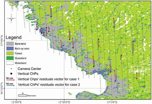
There is a correlation between vertical residual vectors of checkpoints and land cover in the study area. As a partial conclusion in agreement to the antecedent discussion about GCPs (Figures S6 and S7) and the vertical residual vectors for the checkpoints (Figures S8 and 5), besides, the RMS residual of checkpoints for case 1 and case 2 is 0.184 m and 0.157 m (Table 1, for checkpoint RMS of Residual), case 2 is the better solution. It is worth mentioning that it is difficult to make any conclusion on the effect of land cover on horizontal checkpoint residual vectors’ distribution and magnitude because these checkpoints are mostly in bare land and built-up areas and are not well distributed. This limits us to any further conclusion if the forest or water-land have any effect on these residuals.

Comparison of photogrammetric derived DSM and LiDAR data

The obtained digital surface model (DSM) using three best observable uncertainties and together with, the default Lantmäteriet observable uncertainty is evaluated by the national height model of Sweden (Lantmateriet 2020). The three best observable uncertainties are [0.2 m for $E,N,H$ and 0.007$\text{^^circ}$, 0.007$\text{^^circ}$and 0.009$\text{^^circ}$for $\omega ,\phi ,\kappa$], [0.08 m for $E,N,H$ and 0.003$\text{^^circ}$, 0.003$\text{^^circ}$, 0.007$\text{^^circ}$for $\omega ,\phi ,\kappa$] and the combination of them [0.08 m for $E,N,H$ and 0.007$\text{^^circ}$, 0.007$\text{^^circ}$, 0.009$\text{^^circ}$for $\omega ,\phi ,\kappa$].

The photogrammetric DSM of different uncertainties of EOPs was created with semi-global matching (SGM) approach in the nFrames-Sure software (Nframes 2020) and a grid was created with median filtering which the resolution was lowered because of averaging. Ground points in the Terrasolid-Terrascan software (Terrasolid 2020) classified the LiDAR-derived DTM, and a grid was created by the triangulation of the ground points. DSM is a surface model and DTM is a ground model, only objects at the ground (flat area) can be used to estimate absolute accuracy (Dell Acqua et al. 2001). Therefore, a flat area is selected for evaluating the differences between DTM and DSM.

Over the past decade, a notable improvement occurred in the field of generating DTM and DSM by photogrammetric image-matching (Jensen and Mathews 2016). The vertical accuracy of photogrammetric DSM is less than ALS’s (airborne laser scanning) DTM (Hodgson et al. 2003, Rahmayudi and Rizaldy 2016, Simpson et al. 2017). ALS point cloud vertical accuracy is usually reported at approximately 1 ~ 20 cm (Ballhorn et al. 2009, Estornell et al. 2011, Reddy et al. 2015, Konecny et al. 2016). Therefore, in this study, the DTM of LiDAR was selected as the reference and compared with photogrammetric DSMs. Table 2, shows the statistical analysis of the residuals between DTM and DSMs. The road as a flat area is selected for the comparison between DSMs and DTM of LiDAR because these two models have the lowest differences in this specific area. However, some anomaly obviously can be seen in Table 2, which could be due to proportionally covering the road, by some height objects like trees. Nevertheless, the main purpose of this comparison is to show which DSMs (with different uncertainties) are closer to the DTM of LiDAR. The RMS of residuals between DTM and DSMs is not huge in different uncertainties although, the range of differences is 2–4.8 cm relative to the lowest RMS of residuals. All in all, the 0.2 m for $E,N,H$ and 0.007$\text{^^circ}$, 0.007$\text{^^circ}$, 0.009$\text{^^circ}$for $\omega ,\phi ,\kappa$has the best RMS of residual and variance for road patches (flat area).

Table 2. Statistical analysis for elevation differences between LiDAR’s DTM and Photogrammetry DSMs.

GNSS (m)	IMU(${ }^{\circ }$)	Area	Statistical parameters (m)
u(E), u(N), u(H)	u(ω), u(φ), u(κ)		Mean	RMS of residual	Variance
0.2, 0.2, 0.2	0.003, 0.003, 0.007	Road	0.095	1.877	3.522
0.2, 0.2, 0.2	0.007, 0.007, 0.009		0.086	1.832	3.358
0.08, 0.08, 0.08	0.003, 0.003, 0.007		0.053	1.88	3.534
0.08, 0.08, 0.08	0.007, 0.007, 0.009		0.054	1.854	3.438

Conclusion

This paper presents the significance of different GNSS and IMU observable uncertainties on GNSS shift and drift corrections in Aerial Triangulation (AT) and its final accuracy. By assessing the RMS residual of checkpoints in two block-wise and strip-wise scenarios, it can be concluded that the method of block-wise GNSS shift correction is a better procedure for processing the AT for the selected test area. Furthermore, a t-test on different observable uncertainties used, and a set of uncertainties was selected as best and worst cases in the block-wise approach to analyse the residual vectors for making better decisions about the proper uncertainties. Finally, it concluded that 0.2 m for $E,N,H$ and 0.007$\text{^^circ}$, 0.007$\text{^^circ}$ and 0.009$\text{^^circ}$for $\omega ,\phi ,\kappa$, respectively, are the best observable uncertainty values for calculating the AT via fewer numbers of rejected images and relatively smaller RMS residuals of checkpoints. This conclusion is made by examining the differences between the DTM of LiDAR and the DSM derived from photogrammetry for four different observables’ uncertainties.

This specific set of proposed uncertainty worked properly for this specific photogrammetry block and might be different in other test areas with different land cover and measurement parameters (e.g. GCPs and checkpoint measurement’s methods, observable accuracies, distribution of GCPs, quality of obtaining image (GSD), tie-points extraction, etc.) which can directly impact on final results.

After executing a t-test, the images with gross errors could be determined; hence, better results would be achieved if it was possible to change (increase) their GNSS/IMU observable uncertainties for such images with gross errors individually. It was not possible in this study to assign different uncertainties for each image due to the limitation of the software options and therefore, there is our recommendation for solving this issue in further researches.

Acknowledgments

The authors acknowledge the support of the Lars Erik Lundberg Scholarship Foundation for providing the opportunity to do this study. We would like to thank and acknowledge Lantmäteriet for providing the photogrammetric dataset, analysing software and supporting us in this paper. We would also like to show our gratitude to Anders Ekholm, Håkan Ågren, Jesper M. Paasch and Rolf Kulla for sharing their pearls of wisdom with us during the course of this research. We sincerely thank the anonymous reviewers and the editor for their constructive and useful comments that helped us to improve and clarify this manuscript.

Disclosure statement

No potential conflict of interest was reported by the author(s).

Supplementary material

Supplemental data for this article can be accessed here.

Correction Statement

This article has been republished with minor changes. These changes do not impact the academic content of the article.

Additional information

Funding

This work was supported by the Lars Erik Lundbergs Stiftelse för Forskning och Utbildning.

References

- Ballhorn, U., et al., 2009. Derivation of burn scar depths and estimation of carbon emissions with LIDAR in Indonesian peatlands. Proceedings of the National Academy of Sciences, 106 (50), 21213–21218. doi:10.1073/pnas.0906457106
- Baselga, S., 2007. Global optimization solution of robust estimation. Journal of Surveying Engineering, 133 (3), 123–128. doi:10.1061/(ASCE)0733-9453(2007)133:3(123)
- Bjerhammar, A., 1973. A theory of errors and generalized inverse matrices. Amsterdam, New York: Elsevier Scientific Publishing Co.
- Blázquez, M. and Colomina, I., 2012. Relative INS/GNSS aerial control in integrated sensor orientation: models and performance. ISPRS Journal of Photogrammetry and Remote Sensing, 67, 120–133. doi:10.1016/j.isprsjprs.2011.11.003
- Copernicus Europe’s eyes on Earth, 2020. Land monitoring service. Available from: https://land.copernicus.eu/ [Accessed 08 Sep 2020].
- Cramer, M., 1999. Direct geocoding: is aerial triangulation obsolete. In: Fritsch and Spiller, eds. Photographic week 1999. Berline, Germany: Heidelberg Wichmann, 59–70.
- Cramer, M., 2001. Genauigkeitsuntersuchungen zur GPS-INS-Integration in der Aerophotogrammetrie. Verlag der Bayerischen Akademie der Wissenschaften in Kommission bei der C.H. Beck'schen Verlagsbuchhandlung.
- Cramer, M., Stallmann, D., and Haala, N., 2000. Direct georeferencing using GPS/inertial exterior orientations for photogrammetric applications. International Archives of Photogrammetry and Remote Sensing, 33 (B3/1; PART 3), 198–205.
- Dell Acqua, F., Gamba, P., and Mainardi, A., 2001. Digital terrain models in dense urban areas. International Archives of Photogrammetry Remote Sensing and Spatial Information Sciences, 34 (3/W4), 195–202.
- El-Ashmawy, K.L., 2018. Photogrammetric block adjustment without control points. Geodesy and Cartography, 44 (1), 6–13. doi:10.3846/gac.2018.880
- Estornell, J., et al., 2011. Analysis of the factors affecting LiDAR DTM accuracy in a steep shrub area. International Journal of Digital Earth, 4 (6), 521–538. doi:10.1080/17538947.2010.533201
- Gerke, M., 2009. Dense matching in high resolution oblique airborne images. International Archives of Photogrammetry Remote Sensing and Spatial Information Sciences, 38 (3/W4), 77–82.
- Gerke, M., 2011. Using horizontal and vertical building structure to constrain indirect sensor orientation. ISPRS Journal of Photogrammetry and Remote Sensing, 66 (3), 307–316. doi:10.1016/j.isprsjprs.2010.11.002
- Gruen, A., 2012. Development and status of image matching in photogrammetry. The Photogrammetric Record, 27 (137), 36–57. doi:10.1111/j.1477-9730.2011.00671.x
- Gruszczyński, W., Matwij, W., and Ćwiąkała, P., 2017. Comparison of low-altitude UAV photogrammetry with terrestrial laser scanning as data-source methods for terrain covered in low vegetation. ISPRS Journal of Photogrammetry and Remote Sensing, 126, 168–179. doi:10.1016/j.isprsjprs.2017.02.015
- Gülch, E., 2012. Photogrammetric measurements in fixed wing UAV imagery. The International Archives of Photogrammetry, Remote Sensing and Spatial Information Sciences, 39 (B1), 381–386. doi:10.5194/isprsarchives-XXXIX-B1-381-2012
- Heipke, C., 1999. Automatic aerial triangulation: results of the OEEPE-ISPRS test and current developments. Wichmann: Photogrammetric week, 177–191.
- Heipke, C., Jacobsen, K., and Wegmann, H., 2002. Analysis of the results of the OEEPE test “Integrated Sensor Orientation”. In: OEEPE Integrated Sensor Orientation Test Report and Workshop Proceedings, Hannover, Germany, Editors.
- Hodgson, M.E., et al., 2003. An evaluation of LIDAR-and IFSAR-derived digital elevation models in leaf-on conditions with USGS Level 1 and Level 2 DEMs. Remote Sensing of Environment, 84 (2), 295–308. doi:10.1016/S0034-4257(02)00114-1
- Hohle, J., 2008. Photogrammetric measurements in oblique aerial images. Photogrammetrie Fernerkundung Geoinformation, 2008 (1), 7.
- Ip, A., El-Sheimy, N., and Mostafa, M., 2007. Performance analysis of integrated sensor orientation. Photogrammetric Engineering and Remote Sensing, 73 (1), 89–97. doi:10.14358/PERS.73.1.89
- Jensen, J.L. and Mathews, A.J., 2016. Assessment of image-based point cloud products to generate a bare earth surface and estimate canopy heights in a woodland ecosystem. Remote Sensing, 8 (1), 50. doi:10.3390/rs8010050
- Jouybari, A., et al., 2019. Methods comparison for attitude determination of a lightweight buoy by raw data of IMU. Measurement, 135, 348–354.
- Jouybari, A., Ardalan, A.A., and Rezvani, M.H., 2017. Experimental comparison between Mahoney and Complementary sensor fusion algorithm for attitude determination by raw sensor data of Xsens IMU on buoy. The International Archives of the Photogrammetry, Remote Sensing and Spatial Information Sciences, 42, 497–502.
- Kerner, S., Kaufman, I., and Raizman, Y., 2016. Role of Tie-Points distribution in aerial photography. The International Archives of Photogrammetry, Remote Sensing and Spatial Information Sciences, 41–44. doi:10.5194/isprsarchives-XL-3-W4-41-2016
- Kersten, T., Haering, S., and Ag, S.V., 1998. Automatic tie point extraction using the oeepe/isprs test data—the swissphoto investigations. Hamburg: HafenCity Universität Hamburg. (Report for the pilot center of the oeepe/isprs test, Photogrammetrie & Laserscanning).
- Kiraci, A.C. and Toz, G., 2016. Theoretical analysis of positional uncertainty in direct georeferencing. The International Archives of Photogrammetry, Remote Sensing and Spatial Information Sciences, 41 (p), 1221.
- Konecny, K., et al., 2016. Variable carbon losses from recurrent fires in drained tropical peatlands. Global Change Biology, 22 (4), 1469–1480. doi:10.1111/gcb.13186
- Kraus, K., 2007. Photogrammetry – geometry from images and laser scans. 2nd ed. Vienna, Austria: de Gruyter.
- Kruck, E., 2001. Combined IMU and sensor calibration with BINGO-F. In: Integrated Sensor Orientation, Proc. of the OEEPE Workshop, Hannover, Germany, March.
- Lantmateriet, 2020. Elevation data - National elevation model. Available from: https://www.lantmateriet.se/sv/Kartor-och-geografisk-information/geodataprodukter/stodsidor/hojddata—nationell-hojdmodell/# [Accessed 14 Sep 2020].
- Lembicz, B.W., 2006. Minimizing ground control when gps photogrammetry isn’t practical. In: ASPRS 2006 Annual Conference, Reno, Nevada, May, 1–5.
- Madani, M. and Mostafa, M.M.R., 2001. ISAT direct exterior orientation QA/QC strategy using POS data. In: Proceedings of OEEPE Workshop: Integrated Sensor Orientation, September, Hanover, Germany, 17–18.
- Madani, M. and Shkolnikov, I., 2005. Dynamic drift model for GPS/INS post-processed trajectory of frame camera. In: ISPRS Hanover Workshop, Germany.
- Mesas-Carrascosa, F.J., et al., 2014. Positional quality assessment of orthophotos obtained from sensors onboard multi-rotor UAV platforms. Sensors, 14 (12), 22394–22407. doi:10.3390/s141222394
- Mostafa, M.M., Hutton, J., and Lithopoulos, E., 2001a. Airborne direct georeferencing of frame imagery: an error budget. In: Proceedings of the 3rd International Symposium on Mobile Mapping Technology (MMS2001), Cairo, Egypt, January.
- Mostafa, M.R. and Hutton, J., 2001b. Airborne kinematic positioning and attitude determination without base stations. In: Proceedings, International Symposium on Kinematic Systems in Geodesy, Geomatics, and Navigation (KIS 2001), June, Banff, Alberta, Canada.
- Nframes, 2020. Sure aerial - The solution for city and countrywide mapping with aerial imagery. Available from: https://www.nframes.com/products/sure-aerial/ [Accessed 06 Nov 2020].
- Osada, E., 2001. Geodesy. Wrocław: Wroclaw University of Science and Technology Publishing. (In Polish).
- Pfeifer, N., Glira, P., and Briese, C., 2012. Direct georeferencing with on board navigation components of light weight UAV platforms. ISPRS - International Archives of the Photogrammetry, Remote Sensing and Spatial Information Sciences, 39, 487–492. doi:10.5194/isprsarchives-XXXIX-B7-487-2012
- Rahmayudi, A. and Rizaldy, A., 2016. Comparison of semi automatic DTM from image matching with DTM from Lidar. International Archives of the Photogrammetry, Remote Sensing & Spatial Information Sciences, 41, 373–380.
- Reddy, A.D., et al., 2015. Quantifying soil carbon loss and uncertainty from a peatland wildfire using multi-temporal LiDAR. Remote Sensing of Environment, 170, 306–316. doi:10.1016/j.rse.2015.09.017
- Rizaldy, A. and Firdaus, W., 2012. Direct georeferencing: A new standard in photogrammetry for high accuracy mapping. International Archives of the Photogrammetry, Remote Sensing and Spatial Information Sciences, 39, B1.
- Salach, A., et al., 2018. Accuracy assessment of point clouds from LidaR and dense image matching acquired using the UAV platform for DTM creation. ISPRS International Journal of Geo-Information, 7 (9), 342. doi:10.3390/ijgi7090342
- Scherzinger, B.M., 1996. Inertial navigator error models for large heading uncertainty. In: Proceedings of Position, Location and Navigation Symposium-PLANS’96. Atlanta, GA, IEEE, April, 477–484.
- Schmitz, M., et al., 2001. Benefit of Rigorous Modeling of GPS in Combined AT/GPS/IMU-Bundle Block Adjustment. In: OEEPE Workshop on Integrated Sensor Orientation, Organisation Europene d’Etudes Photogrammtriques Exprimentales/European Organization for Experimental Photogrammetric Research (OEEPE), Hannover, September.
- Seifert, E., et al., 2019. Influence of drone altitude, image overlap, and optical sensor resolution on multi-view reconstruction of forest images. Remote Sensing, 11 (10), 1252. doi:10.3390/rs11101252
- Serifoglu, C., Gungor, O., and Yilmaz, V., 2016. Performance evaluation of different ground filtering algorithms for UAV-based point clouds. International Archives of the Photogrammetry, Remote Sensing & Spatial Information Sciences, 41, 245–251.
- Shi, J., et al., 2017. GPS real-time precise point positioning for aerial triangulation. GPS Solutions, 21 (2), 405–414. doi:10.1007/s10291-016-0532-2
- Simpson, J.E., Smith, T.E., and Wooster, M.J., 2017. Assessment of errors caused by forest vegetation structure in airborne LiDAR-derived DTMs. Remote Sensing, 9 (11), 1101. doi:10.3390/rs9111101
- Snavely, N., Seitz, S.M., and Szeliski, R., 2008. Modeling the world from internet photo collections. International Journal of Computer Vision, 80 (2), 189–210. doi:10.1007/s11263-007-0107-3
- Stöcker, C., et al., 2017. Quality assessment of combined IMU/GNSS data for direct georeferencing in the context of UAV-based mapping. The International Archives of Photogrammetry, Remote Sensing and Spatial Information Sciences, 42, 355.
- Terrasolid, 2020. TerraScan – software for LiDAR data processing and 3D vector data creation. Available from: http://www.terrasolid.com/products/terrascanpage.php [Accessed 06 Nov 2020].
- Tomaštík, J., et al., 2017. Accuracy of photogrammetric UAV-based point clouds under conditions of partially-open forest canopy. Forests, 8 (5), 151. doi:10.3390/f8050151
- Triggs, B., et al., 1999. Bundle adjustment—a modern synthesis. In: International workshop on vision algorithms, September. Berlin, Heidelberg: Springer, 298–372.
- Trimble, 2015. MATCH-AT reference manual. Germany: Trimble inpho.
- Truong Giang, N., et al., 2018. Second iteration of photogrammetric processing to refine image orientation with improved tie-points. Sensors, 18 (7), 2150. doi:10.3390/s18072150
- Tsai, V.J., Kao, J.S., and Chen, C.N., 2006. On GPS and GPS-RTK assisted aerotriangulation. In: Proceedings of ASPRS 2006 Annual Conference. Reno, Nevada: ASPRS, 1–10.
- Wallace, L., et al., 2016. Assessment of forest structure using two UAV techniques: A comparison of airborne laser scanning and structure from motion (SfM) point clouds. Forests, 7 (3), 62. doi:10.3390/f7030062
- Wierzbicki, D., 2017. Determination of Shift/Bias in digital aerial triangulation of UAV imagery sequences. In: IOP Conference Series: Earth and Environmental Science Vol. 95, No. 3, December. Prague, Czech Republic, IOP Publishing, 032033.
- Xie, L., et al., 2016. An asymmetric re-weighting method for the precision combined bundle adjustment of aerial oblique images. ISPRS Journal of Photogrammetry and Remote Sensing, 117, 92–107. doi:10.1016/j.isprsjprs.2016.03.017
- Yastikli, N., Toth, C., and Grejner-Brzezinska, D.A., 2007. In-situ camera and boresight calibration with LiDAR Data. In: Proc. The Fifth International Symposium on Mobile Mapping Technology, MMT, Padua, Italy, Vol. 7.
- Yuan, X., et al., 2009. The application of GPS precise point positioning technology in aerial triangulation. ISPRS Journal of Photogrammetry and Remote Sensing, 64 (6), 541–550. doi:10.1016/j.isprsjprs.2009.03.006
- Zach, C., 2014. Robust bundle adjustment revisited. In: European Conference on Computer Vision, September. Cham: Springer, 772–787.
- Zhang, Y., Hu, B., and Zhang, J., 2011. Relative orientation based on multi-features. ISPRS Journal of Photogrammetry and Remote Sensing, 66 (5), 700–707. doi:10.1016/j.isprsjprs.2011.06.001