Quantifying rates of soil deflation with Structure-from-Motion photogrammetry in west Greenland

ABSTRACT

Aeolian processes are important drivers of geomorphic change in cold regions. Because these processes often occur at slow timescales over large areas, it can be difficult to quantify rates using traditional field methods. In the Kangerlussuaq region of Greenland, strong katabatic winds have shaped distinct erosional landforms, or deflation patches, that appear to expand across the landscape. The modern erosion rate along the active margins, or scarps, of these deflation patches is unknown. We use Structure-from-Motion (SfM) photogrammetry to quantify the geomorphic change of ten deflation patches between 2014 and 2016. During the two-year study period, significant positive and negative change occurred at all sites, suggesting that deflation patches are active landforms and that geomorphic change is highly heterogeneous and localized. We observed significant change primarily along the scarps, while little to no change occurred in the center of the patches. Along the scarps, the mean negative change ranged from −0.7 to −2.5 cm, and erosion dominated in eight out of the ten deflation patches. The modern erosion rate appears to be lower than the century-scale rate of 2.5 cm yr⁻¹ estimated from prior work using lichenometry, potentially because of the episodic nature of scarp retreat. Longer-term monitoring using these methods will help quantify the geomorphic response of this landscape to a rapidly changing regional climate.

KEYWORDS:

• Photogrammetry
• Structure-from-Motion
• soil erosion
• Arctic
• aeolian processes

Introduction

Aeolian processes are important drivers of geomorphic change in polar regions, where there is often little shelter from strong winds. Because of the slow timescales and large spatial impacts of these processes, rates of aeolian erosion and deposition can be difficult to quantify using traditional field methods. While aeolian processes are well studied in some Arctic locations, such as Iceland (e.g., Arnalds, Dagsson-Waldhauserova, and Olafsson 2016), most polar regions are frequently overlooked, even though these landscapes are often susceptible to soil erosion and contribute significantly to the global dust budget (Bullard 2013; Bullard et al. 2016). Establishing baseline rates of soil erosion is especially important in the Arctic, where rapid environmental change is resulting in altered wind dynamics, permafrost thaw, and coastline collapse (IPCC 2013).

Kangerlussuaq, southern west Greenland, is one such Arctic location where modern rates of soil erosion are unknown. Erosional landforms, here referred to as deflation patches, cover roughly 22 percent of the terrestrial landscape in the Kangerlussuaq region (Heindel, Chipman, and Virginia 2015). These distinct bare patches range in size from tens to hundreds of square meters and form when strong katabatic winds off the Greenland Ice Sheet (GrIS) remove vegetation, soil, and underlying loess, exposing glacial till and bedrock. Although deflation patches are generally low in biomass, they provide habitat for biological soil crusts (biocrusts), assemblages of lichens, mosses, algae, fungi, and other microorganisms (e.g., Weber, Büdel, and Belnap 2016). Deflation patches are bounded on the downwind side by a sharp erosional front, or scarp, that moves across the landscape (Heindel, Culler, and Virginia 2017). These scarps are often undercut, and deflation patches expand when blocks of soil and vegetation collapse. Modern and future rates of deflation-patch expansion have important consequences for ecosystem productivity, vegetation distributions, nutrient cycling, and aquatic environments (e.g., Anderson et al. 2017; Perren et al. 2012; Petrenko et al. 2016).

Although modern rates of soil erosion are unknown, deflation-patch expansion during the past 425 years has been estimated to be 2.5 cm yr⁻¹ using lichenometry (Heindel, Culler, and Virginia 2017). In that prior study, rates of patch expansion were found to be similar among patches and did not correlate with proximity to the GrIS, aspect, or slope. While the century-scale estimates suggest that erosion rates have been relatively constant throughout the past 425 years, the coarse resolution and high uncertainty of lichenometry make it difficult to estimate modern erosion rates using this method.

While traditional survey techniques (e.g., total station or Real Time Kinematic [RTK]-GPS) are useful, we chose to quantify geomorphic change at deflation patches using digital photogrammetry to achieve high accuracy without disturbing the patches. Digital photogrammetry provides an efficient and limited-contact method to quantify rates of change during short time periods and to map the distributions of geomorphic change at fine spatial scales. During the past decade, the development of Structure-from-Motion (SfM) and multi-view stereo photogrammetry has enabled the modeling of 3-D objects and landforms using highly overlapping sets of photographs (Fonstad et al. 2013; James and Robson 2012; Javemick, Brasington, and Caruso 2014; Westoby et al. 2012). In this method, orienting the raw images and constructing a dense 3-D point cloud is largely automated, allowing for the collection and processing of large amounts of high-resolution topographic data.

To quantify geomorphic change at deflation patches, our photogrammetry methods needed to handle complex topography and be accurate on the millimeter-to-centimeter scale. Several recent studies demonstrate the ability of SfM to create high-resolution models of landforms and vegetation in polar environments using imagery acquired from unmanned aerial vehicles (UAVs; e.g., Lucieer et al. 2014; Westoby et al. 2015). For instance, Westoby et al. (2015) used UAV-SfM to quantify the grain size of moraine sediment and achieved millimeter-scale accuracy. Terrestrial, or ground-based, photography can also be used to acquire imagery for SfM as an effective way to monitor small areas. In this study, we used terrestrial SfM to capture the complex and often overhanging topography of deflation patches and to avoid the potential systematic distortions that can result from the parallel camera geometry used in most UAV flight plans (Carbonneau and Dietrich 2017; James and Robson 2014). The use of terrestrial SfM to quantify soil erosion at the centimeter scale has been demonstrated in both field and lab settings (Rieke‐Zapp and Nearing 2005; Heng, Chandler, and Armstrong 2010; Mayr et al. 2016).

Here we use terrestrial SfM to estimate rates of scarp retreat between 2014 and 2016 and to test several theories about deflation-patch expansion. First, we test whether deflation patches are currently active by quantifying geomorphic change during a short two-year time interval. Second, we consider the processes that lead to deflation-patch expansion and scarp retreat by determining spatial patterns of erosion. Finally, we compare modern erosion rates to the century-scale estimate of 2.5 cm yr⁻¹. The results of this analysis provide insight into the ongoing role of aeolian soil erosion in shaping the Kangerlussuaq landscape. More broadly, the study highlights the use of high-resolution 3-D photogrammetry as a powerful tool for research in ecology and geomorphology.

Methods

Study area

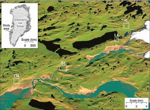
Our study area extended from the town of Kangerlussuaq to the margin of the Russell Glacier, an outlet glacier of the GrIS (Figure 1). From the margin of the GrIS to the town of Kangerlussuaq, wind speeds diminish and wind directions conform to local topography (Bullard and Austin 2011; Dijkmans and Törnqvist 1991). Vegetation transitions from a mixture of graminoids and prostrate shrubs close the GrIS to a mixture of deciduous shrubs dominated by Salix glauca close to town (Heindel, Chipman, and Virginia 2015). To capture these gradients in climate and land cover, we established four study sites within the Kangerlussuaq region, listed in increasing proximity to the GrIS: Town, Sugarloaf, Long Lake, and Inland (Figure 1). These sites are part of a larger effort to understand the extent, age, and impact of deflation patches, using techniques such as lichenometry and satellite remote sensing (Heindel et al., 2015; Heindel, Culler, and Virginia 2017). For the purposes of this study, we chose ten deflation patches for photogrammetric analysis: two at Town, four at Sugarloaf, two at Long Lake, and two at Inland (Table 1). To limit the number of photographs required, the deflation patches selected for this study were relatively small (37–128 m²) and distinct from the surrounding tundra (Table 1).

Table 1. Locations and details for the ten deflation patches

Patch ID	Latitude	Longitude	Elevation (m)	Area (m^2)	Date of First	Date of Second	Number of Photos (2014, 2016)
ILGRID1	67.11111	−50.25259	366	92.0	01-07-2014	08-07-2016	59, 54
ILSCARP18	67.11276	−50.25615	391	128.3	03-07-2014	08-07-2016	74, 54
LLGRID5	67.08790	−50.29526	280	47.8	24-06-2014	29-06-2016	63, 43
LLGRID6	67.08782	−50.29544	283	84.3	24-06-2014	29-06-2016	78, 48
SLGRID1	67.03974	−50.53759	146	91.2	30-06-2014	02-07-2016	80, 47
SLGRID2	67.03876	−50.53415	130	87.3	30-06-2014	02-07-2016	56, 37
SLSCARP9	67.03641	−50.54607	154	59.2	06-07-2014	02-07-2016	52, 28
SLSCARP10	67.03696	−50.54942	171	36.9	06-07-2014	02-07-2016	55, 34
TNGRID2	67.01474	−50.75369	275	108.9	22-06-2014	02-07-2016	82, 39
TNGRID4	67.01700	−50.75092	333	118.1	08-07-2014	02-07-2016	75, 59

Figure 1. Map showing the locations of the study sites near Kangerlussuaq, Greenland. TN = Town, SL = Sugarloaf, LL = Long Lake, IL = Inland. For coordinates of study sites, see Table 1. Background is a Landsat-7 image from 2000, courtesy USGS

Field data collection and local coordinate system

We photographed the ten deflation patches during the summers of 2014 and 2016. At each deflation patch, we collected a densely overlapping set of photographs (5284 × 3456 8-bit RGB pixels) using a handheld Canon EOS 60D digital camera with an 18–135 mm zoom lens fixed at 18 mm (Table 1, Figures 2 and 3).

Figure 2. Four terrestrial photographs of soil deflation patch LLGRID5. Note the scarp, visible in all photos. For scale, the ground control mat is roughly 38 × 44 cm. Photos taken June 24, 2014

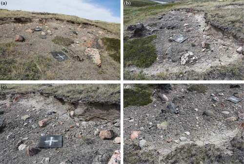
Figure 3. Establishment of a local coordinate system for deflation patch LLGRID5. Top: Textured model of patch with camera locations superimposed in blue; distances among three control points in white. Bottom: Resulting coordinate system with origin at point A and x axis along segment AB

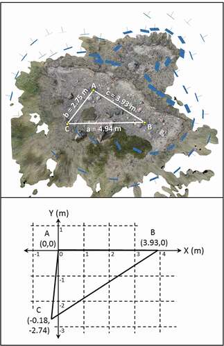
To scale our SfM models (Fonstad et al. 2013; Javemick, Brasington, and Caruso 2014), we established a local coordinate system in 2014 for each deflation patch by measuring straight-line distances among three ground control points (Figure 3). We defined the first control point (A) as (0,0) and the second control point (B) as (X,0), where X was the measured distance between (A) and (B). We calculated the (X,Y) coordinates for the third control point (C) trigonometrically based on its distances from the previous two points. The Z coordinates for all ground control points were set to 0, regardless of actual elevation differences among the control points. The use of these local coordinate systems resulted in models that were scaled correctly, but whose orientations in the X, Y, and Z axes were inherently arbitrary, rotated relative to north, and tilted relative to the horizontal. In this case, an arbitrary coordinate system was sufficient and allowed for rapid data collection in the field.

Construction of point clouds and 3-D models

We used Agisoft Photoscan Professional (version 1.2.6) to construct point clouds from the raw digital photographs. After we manually masked out background areas and sky, the software performed an initial photo alignment by first identifying matching points within overlapping areas of photographs and then using those points to establish the relative orientation of the photographs (Wolf, Dewitt, and Wilkinson 2014).

For the 2014 models, we manually marked and defined the ground control points in all photographs to scale and rotate each model to fit its local coordinate system. To align the 2016 model to the same coordinate system, we used from four to eight landscape features (often fine-scale patterns on rocks) easily identified in both sets of photographs that we assumed had not moved during the two-year interval (Table 2). We estimated a total registration error between the two models, calculated as the 3-D root mean square error of all of the points used to align the models. Registration errors ranged from 0.4 to 1 cm (Table 2).

Table 2. Tie points and registration error between the 2014 and 2016 models for each site

Patch ID	Number of Tie Points	Registration Error (cm)	Registration Error Used (cm)
ILGRID1	8	0.99	1.0
ILSCARP18	6	0.95	1.0
LLGRID5	7	0.96	1.0
LLGRID6	6	0.65	1.0
SLGRID1	5	0.76	1.0
SLGRID2	5	0.46	0.5
SLSCARP9	4	0.28	0.5
SLSCARP10	5	0.59	1.0
TNGRID2	6	1.00	1.0
TNGRID4	6	0.54	1.0

To build the dense point cloud, the software used a matching algorithm to identify a dense set of matching points among the overlapping photographs in the model and to compute their coordinates via space intersection (Wolf, Dewitt, and Wilkinson 2014; Figure 3).

Change detection

We used an algorithm called Multiscale Model to Model Cloud Comparison (M3C2; Lague, Brodu, and Leroux 2013), implemented in the software CloudCompare (Girardeau-Montaut 2017), to detect change between the 2014 and 2016 point clouds. M3C2 handles complex topography by operating directly on point clouds and by computing change along the direction normal (perpendicular) to the surface. We first subsampled both point clouds to 1 cm and calculated normals for the 2014 model (using a quadric local surface model and minimum spanning tree, knn = 6). Within M3C2, we selected a projection scale of 5 cm, defining the diameter of a cylinder oriented perpendicular to the local surface, within which points were sampled. We set the maximum length of the cylinder to 10 cm, because we did not anticipate geomorphic change to be greater than 10 cm. Within each cylinder, the algorithm computed distance along the normal direction as the median, and surface roughness as the interquartile range, of the points sampled.

Spatial patterns of change

To look at spatial patterns of geomorphic change within deflation patches, we manually segmented each patch into scarp and center zones, using the 2016 dense point cloud. For each zone, we calculated the percentage of points that experienced significant positive and negative change, as defined further on. We also report mean values for points that experienced positive change, points that experienced negative change, and all points within each zone.

Finally, we identified examples of vegetation and biocrust change that were captured within our 3-D models. At four patches, our photographs captured distinct deciduous shrubs growing within the deflation patches. At two patches, our photographs captured instances of biocrust disturbance. We present the examples of vegetation and biocrust change purely as proof of method.

Sources of uncertainty

The main sources of uncertainty in this method are the field measurements of distances between ground control points and the alignment errors between the 2014 and 2016 models. Distances between ground control points are used to set the scale for each model, and the impact of measurement error is proportional to the ratio of the error to the true distance. In our field measurements, the net effect of all components of error in tape measurement should be less than 4 cm (Schofield and Breach 2007). Given the typical 4 m distance between ground control points, this yields an error in model scaling of 1 percent or less.

We quantified the uncertainty in the alignment between the 2014 and 2016 models as the registration error described earlier, which ranged from 0.4 to 1 cm (Table 2). To understand how this registration error impacted our change detection, we performed the same alignment process between our original 2014 model and a duplicate 2014 model created from a subset of photos (fifty-two out of the original seventy-eight) for one deflation patch (LLGRID6). With four tie-points between the models, our registration error was 0.7 cm, within the range of registration errors for the alignment of the 2014 and 2016 models. We then used the CloudCompare analytical process described earlier to quantify the difference between the “no-change” pair of 2014 models due to poor model alignment.

To assess the significance of surface changes, the M3C2 algorithm uses the patch-specific registration error (Table 2) in combination with the measured surface roughness to calculate a 95 percent confidence interval for the change at each point (Lague, Brodu, and Leroux 2013). Where the 95 percent confidence interval does not include zero, change is considered significant. Significance thresholds for the scarp and center zones for each deflation patch ranged from 0.5 to 2.2 cm (Table 3).

Table 3. Significance thresholds for scarp and center zones for each patch. The significance threshold was calculated in M3C2 using the registration error unique to each patch and the local surface roughness

Patch ID	Significance Threshold (cm)
	Scarp	Center
ILGRID1	2.1	1.9
ILSCARP18	1.9	1.5
LLGRID5	1.8	2.2
LLGRID6	1.9	1.9
SLGRID1	1.9	1.9
SLGRID2	1.0	0.9
SLSCARP9	0.8	0.5
SLSCARP10	2.1	2.0
TNGRID2	1.4	1.9
TNGRID4	1.9	1.9

Results

Soil erosion

Patterns of geomorphic change between the 2014 and 2016 point clouds suggest that deflation patches are active landforms and that erosion is highly localized. Significant change was concentrated along the scarps, while little to no significant change occurred within the centers of patches (Figure 4, Table 4). Within scarp zones, the percentage of points that experienced significant negative change ranged from 2.4 to 19.1 and averaged (± standard error) 8.8 (± 1.7). In center zones, significantly less negative change occurred (p = 0.002, two-tailed t test), with the percentage of points that experienced significant negative change ranging from 0.3 to 3.8 and averaging 1.2 (± 0.4).

Table 4. Percentages of points experiencing significant positive and negative change for each zone at all deflation patches. Averages across sites are reported as mean ± standard error

	Scarp		Center
Patch ID	% Points Significant Negative Change	% Points Significant Positive Change	% Points Significant Negative Change	% Points Significant Positive Change
ILGRID1	6.9	9.1	2.5	1.0
ILSCARP18	14.0	2.1	0.4	0.1
LLGRID5	2.4	1.9	0.4	0.7
LLGRID6	19.1	0.2	0.2	0.1
SLGRID1	8.9	2.4	1.4	2.0
SLGRID2	10.9	7.2	0.8	0.2
SLSCARP9	4.6	6.0	0.7	0.1
SLSCARP10	5.7	2.9	3.8	0.1
TNGRID2	2.5	0.2	0.3	0.6
TNGRID4	12.6	11.4	1.7	1.4
Average	8.8 ± 1.7	4.3 ± 1.2	1.2 ± 0.4	0.6 ± 0.2

Figure 4. Results of M3C2 change detection for the scarp and center zones from two deflation patches, ILSCARP18 (A, C, E, G), and LLGRID6 (B, D, F, H). From top to bottom, the rows show (1) the shapes of the scarp and center zones superimposed on the 2014 point clouds (A–B), (2) the spatial distribution of significant change in green (C–D), (3) the magnitude of change between the 2014 and 2016 point clouds (E–F), and (4) histograms of measured change for the scarp (black) and center (gray) zones (G–H)

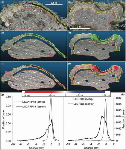
For both scarp and center zones, significant change was spatially heterogeneous with both positive and negative change occurring (Table 4). Although we observed less overall change within center zones, we observed similar proportions of negative to positive change. For both scarp and center zones, roughly two-thirds of significant change was negative (Table 4).

Scarp zones experienced a higher magnitude of change than center zones across all three mean values reported (Table 5). Mean values for five out of the ten scarp zones crossed the significance threshold for either negative or positive change, while no mean values crossed the significance threshold within center zones (Table 5). Across all patches, the distribution of change measured in the scarp zone was wider than in the center zone (Figure 4, Table 5). Standard deviations for individual scarp zones ranged from 1.0 to 3.7 cm, while standard deviations for individual center zones ranged from 0.4 to 1.4 cm (Table 5). In this case, standard deviation is a measure of the spread of the data, rather than a measurement of uncertainty around the mean.

Table 5. Magnitude of change detected for scarp and center zones for all deflation patches. For each zone, we report the mean negative change, the mean positive change, the mean for all points, and the standard deviation for all points. Asterisks mark mean values that exceed the significance threshold reported in Table 3. Averages across patches are reported as mean ± standard error

	Scarp				Center
Patch ID	Mean Negative Change (cm)	Mean Positive Change (cm)	Mean Change of All Points (cm)	Standard Deviation of All Points (cm)	Mean Negative Change (cm)	Mean Positive Change (cm)	Mean Change of All Points (cm)	Standard Deviation of All Points (cm)
ILGRID1	−1.5	2.0	0.2	2.6	−0.8	0.6	−0.1	1.4
ILSCARP18	−1.8	1.0	−1.0	2.2	−0.4	0.2	−0.2	0.5
LLGRID5	−0.9	1.0	−0.1	1.3	−0.4	0.5	0.1	0.7
LLGRID6	−1.9*	0.5	−1.5	2	−0.4	0.3	−0.2	0.5
SLGRID1	−2.1*	1.7	−1.2	2.9	−0.8	0.8	−0.3	1.2
SLGRID2	−1.4*	1.1*	−0.3	2.2	−0.3	0.3	0	0.4
SLSCARP9	−0.7	0.9*	0.1	1.3	−0.3	0.2	0	0.4
SLSCARP10	−1.2	1.2	−0.4	1.9	−1	0.2	−0.3	1.1
TNGRID2	−0.9	0.5	−0.6	1	−0.4	0.5	0.1	0.7
TNGRID4	−2.5*	2.4*	−0.3	3.7	−0.7	0.7	−0.3	1.2
Average	−1.5 ± 0.2	1.2 ± 0.2	−0.5 ± 0.2	2.1 ± 0.3	−0.6 ± 0.1	0.4 ± 0.1	−0.1 ± 0.05	0.8 ± 0.1

We use the mean change of all points along the scarp zone divided by our two-year time interval to compare to the lichenometry estimate of −2.5 cm yr⁻¹. We acknowledge that the annual retreat rates presented here are below our significance thresholds; we use this annual retreat rate only to compare to the century-scale lichenometry estimate. From this study, average annual scarp retreat rates ranged from −0.75 (± 1.0) to +0.1 (± 1.3) cm and averaged −0.25 (± 0.3) cm, a full order of magnitude lower than −2.5 cm yr⁻¹. Three deflation patches—ILSCARP18, LLGRID6, and SLGRID1—experienced more extreme erosion along the scarp than the other deflation patches. These three scarps had annual retreat rates of −0.5 (± 1.1), −0.75 (± 1.0), and −0.6 (± 1.5) cm, respectively. While still less than 2.5 cm yr⁻¹, the retreat rates for these deflation patches are well within the range of rates estimated using lichenometry (Heindel, Culler, and Virginia 2017). Erosion along the scarp was especially noticeable at LLGRID6, where the scarp was more undercut than at any other deflation patch. Here, erosion occurred most severely where the scarp was already undercut, further destabilizing the overhanging block of soil and vegetation (Figure 5).

Figure 5. Examples of negative and positive change along two scarps, LLGRID6 (A, C, E) and ILGRID1 (B, D, F). From top to bottom, the rows show (1) the 2014 point clouds, with the locations of the cross-sections in white (A–B); (2) the magnitude of change between the 2014 and 2016 point clouds (C, D); and (3) cross-sections through the 2014 (green) and 2016 (orange) point clouds (E, F)

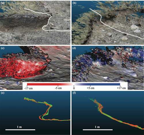
The two deflation patches that experienced more positive than negative change within the scarp zone (ILGRID1 and SLSCARP9) provided examples of the positive change that occurred along scarps between 2014 and 2016. A cross section through the scarp of ILGRID1 (Figure 5) shows that the positive change is associated with a very noisy region of the point cloud, characteristic of vegetated areas. As scarps develop over time, vegetation may start to slump into the deflation patch or grow directly out of the scarp.

Model alignment test

In our test to establish the impact of model alignment on the calculation of surface change, there was virtually no difference between the two 2014 models for LLGRID6. In the center zone, only 0.06 percent of points were above the significance threshold, compared to 0.3 percent for the 2014–2016 model comparison at the same site. More importantly, in the scarp zone, only 0.4 percent of points were above the significance threshold in the 2014–2014 test, far fewer than the 19.3 percent of points that experienced significant change in the 2014–2016 comparison. This exercise gives us confidence that our results reflect real geomorphic change and are not artifacts of poor point-cloud alignment.

Vegetation change

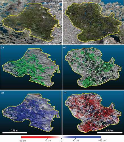
Each of the four shrubs examined showed a consistent direction of change throughout the entire area of the shrub (Figure 6). If we were detecting random changes in the position and orientation of stems and foliage, we would expect to see a random scattering of positive and negative change within an individual shrub. Three of the four shrubs (at LLGRID5, LLGRID6, and TNGRID4) experienced negative change between 2014 and 2016, while one shrub (at ILGRID1) was larger in 2016 than in 2014. The average differences between 2014 and 2016 were −2.1 (± 3.1), −1.7 (± 3.1), −2.0 (± 4.2), and +2.3 (± 2.5) cm for LLGRID5, LLGRID6, TNGRID4, and ILGRID1, respectively. These averages are right below (LLGRID5, LLGRID6) or above (TNGRID4, ILGRID1) the significance threshold for the center zones at these patches (Table 3). We may have captured positive change at ILGRID1 because of the timing of our photography: at this site the second set of photographs was taken one week later (July 8) than the first (July 1). For the other sites, the second set of photographs was either taken close to or earlier than the seasonal date of the first set of photographs. We present these results to demonstrate that terrestrial SfM is a promising method to detect small-scale changes in vegetation in the Arctic, a region currently experiencing the encroachment of deciduous shrubs into graminoid habitats (e.g., Myers-Smith et al. 2011).

Figure 6. Examples of vegetation change from ILGRID1 (A, C, E) and LLGRID5 (B, D, F). From top to bottom, the rows show (1) the Betula nana shrubs and outlines (A–B), (2) the spatial distribution of significant change in green (C–D), and (3) the magnitude of change between the 2014 and 2016 point clouds (E, F)

Biocrust change

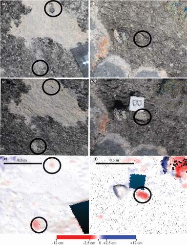
Our methods were able to detect change even at the small scale of biocrust disturbance (Figure 7). At SLSCARP9 and SLSCARP10, we observed areas <50 cm² in extent where the biocrust had been disturbed between 2014 and 2016. Because biocrusts are cohesive and take a long time to develop, biocrust disturbances can lead to persistent depressions in the ground surface. At both SLSCARP9 and SLSCARP10, the M3C2 algorithm detected negative change at the disturbed areas, averaging −0.9 cm (above the significance threshold for SLSCARP9 but below the threshold for SLSCARP10). We present these results to illustrate the potential for terrestrial photogrammetry to be used in studying biocrusts.

Figure 7. Examples of biological soil crust change from SLSCARP9 (A, C, E) and SLSCARP10 (B, D, F). From top to bottom, the rows show (1) the 2014 point clouds, circles highlight areas of interest (A–B); (2) the 2016 point clouds (C–D); and (3) the magnitude of change between the 2014 and 2016 point clouds (E–F)

Discussion

Our results show that terrestrial photogrammetry can be used to quantify geomorphic change in complex topography on fine spatial and temporal scales. With only two years between point clouds, our results provide evidence that deflation patches are active landforms and that aeolian soil erosion is ongoing in the Kangerlussuaq region. Our methods, which include the use of an arbitrary local coordinate system and high-contrast ground control points, are low-cost, quick, and appropriate for remote and/or harsh field conditions. We provide examples of how our methods are applicable not only to geomorphic change associated with soil erosion, but also to vegetation change and biocrust disturbance.

Although our results contain uncertainty from errors in field measurement and model alignment, we were able to detect significant change at all deflation patches using the M3C2 significance threshold calculated from the patch-specific registration error and surface roughness (Lague, Brodu, and Leroux 2013). Based on our duplicate 2014 model comparison and on our ability to detect millimeter-scale biocrust disturbances, we believe that the significance threshold calculated by M3C2 is a conservative estimate. Like other recent studies, our results demonstrate the ability of SfM photogrammetry to detect land-surface and vegetation change at the centimeter and millimeter scales (e.g., Fraser et al. 2016; Westoby et al. 2015).

The average rate of change along scarps estimated in this study (0.25 cm yr⁻¹) was much lower than the century-scale 2.5 cm yr⁻¹ lichenometry estimate (Heindel, Culler, and Virginia 2017). Many factors may explain this discrepancy. First, scarps retreat because of the combined effect of scarp undercutting and intermittent scarp collapse. While the lichenometry methods used in Heindel, Culler, and Virginia (2017) captured both processes, this study captured only the process of scarp undercutting due to the short two-year time interval. Second, the spatial heterogeneity of geomorphic change may have contributed to the discrepancy. Averaging rates of change across the entire scarp zone allows positive and negative change to cancel out, resulting in low estimates of total change. Finally, the different climate conditions experienced during the two study periods may also explain the discrepancy between the two estimates. Although the lichenometry study suggested that erosion rates have remained relatively constant throughout the past 425 years, the coarse resolution of lichenometry may not allow for the detection of small changes in erosion rates. During the colder, drier, and windier conditions of the so-called Little Ice Age, scarp retreat may have been more rapid (Aebly and Fritz 2009; D’Andrea et al. 2011; O’Brien et al. 1995).

The spatial patterns of geomorphic change that we observed support the theory that scarps are the most active regions of deflation patches. As expected, most of the change along scarps was erosional, and we observed the process of scarp undercutting that eventually leads to scarp collapse. One unanticipated result was the amount of positive change that also occurred along scarps. Although positive change is often interpreted as deposition, we do not believe that aeolian sediments accumulated along scarps during our study period. Instead, we attribute the positive change to slumping, biocrust development, and vegetation growth directly out of the scarp. Regions along scarps with positive change tended to have considerable noise in the point cloud, characteristic of vegetation. Over time, slumping may decrease the angle of the scarp and reduce the likelihood of scarp failure. Biocrust development and vegetation growth protect soil from winds. Together, these processes may stabilize the scarp and prevent future erosion.

The co-occurrence of positive and negative change within scarp zones highlights the two trajectories that deflation patches may follow in the future. On the one hand, we see evidence for scarp undercutting and retreat, a process that will allow the bare and unproductive patches to continue expanding into the shrub and graminoid tundra. On the other hand, we also see evidence for scarp stabilization through slumping, biocrust development, and vegetation growth. In this case, vegetation may encroach into the deflation patches, reclaiming bare ground. Currently, erosion outpaces stabilization, with eight out of ten deflation patches experiencing net erosion along scarps. In the future, if evapotranspiration increases because of warming summer temperatures (Hanna et al. 2012), climate conditions may favor soil erosion. In this study, we establish an important baseline rate of soil deflation in the Kangerlussuaq region, allowing for future longer-term monitoring.

Conclusions

Deflation patches, common erosional features in the Kangerlussuaq region of southern west Greenland, are active landforms that experienced significant geomorphic change from 2014 to 2016. Geomorphic change occurred primarily along the scarps, while the center of deflation patches, where biocrusts stabilize the soil surface, experienced little significant change. Along the scarps, we observed evidence of both deflation-patch expansion and stabilization. Over all, eight out of ten scarps experienced net erosion, and mean values for negative change ranged from −0.7 to −2.5 cm along scarps. However, positive change occurred as well, likely because of slumping, biocrust development, and vegetation growth. Mean values for positive change along scarps ranged from 0.5 to 2.4 cm. While the modern erosion rate appears to be lower than the century-scale estimate of 2.5 cm yr⁻¹, this discrepancy may be explained by the episodic nature of scarp retreat, spatial variability in geomorphic change, and the different climate conditions during the two study periods. We establish an important baseline of soil erosion in the Kangerlussuaq region. Longer-term monitoring using photogrammetry will help quantify geomorphic response to a rapidly changing regional climate. More broadly, this study highlights the use of terrestrial photogrammetry as a powerful tool in the study of ecological and geomorphic change.

Acknowledgments

We thank Kangerlussuaq International Science Support and Polar Field Services for field logistics. Becca Novello, Phoebe Racine, and Angela Spickard assisted with field methods and data collection. We thank Bob Hawley for use of laboratory facilities.

Additional information

Funding

This research was supported in part by NSF IGERT award #0801490 to RAV.

References

- Aebly, F. A., and S. C. Fritz. 2009. Palaeohydrology of Kangerlussuaq (Søndre Strømfjord), West Greenland during the last ~8000 years. The Holocene 19:1–13. doi:https://doi.org/10.1177/0959683608096601.
- Anderson, N. J., J. E. Saros, J. E. Bullard, S. M. P. Cahoon, S. McGowan, E. A. Bagshaw, C. D. Barry, R. Bindler, B. T. Burpee, J. L. Carrivick, et al. 2017. The Arctic in the twenty-first century: Changing biogeochemical linkages across a paraglacial landscape of Greenland. BioScience 67:118–33.
- Arnalds, O., P. Dagsson-Waldhauserova, and H. Olafsson. 2016. The Icelandic volcanic aeolian environment: Processes and impacts—A review. Aeolian Research 20:176–95. doi:https://doi.org/10.1016/j.aeolia.2016.01.004.
- Bullard, J. E. 2013. Contemporary glacigenic inputs to the dust cycle. Earth Surface Processes and Landforms 38:71–89. doi:https://doi.org/10.1002/esp.v38.1.
- Bullard, J. E., and M. J. Austin. 2011. Dust generation on a proglacial floodplain, west Greenland. Aeolian Research 3:43–54. doi:https://doi.org/10.1016/j.aeolia.2011.01.002.
- Bullard, J. E., M. Baddock, T. Bradwell, J. Crusius, E. Darlington, D. Gaiero, S. Gasso, G. Gisladottir, R. Hodgkins, R. McCulloch, et al. 2016. High-latitude dust in the earth system. Reviews of Geophysics 54:447–85. doi:https://doi.org/10.1002/2016RG000518.
- Carbonneau, P. E., and J. T. Dietrich. 2017. Cost-effective non-metric photogrammetry from consumer-grade sUAS: Implications for direct georeferencing of structure from motion photogrammetry. Earth Surface Processes and Landforms. 42:473–86. doi:https://doi.org/10.1002/esp.4012.
- D’Andrea, W. J., Y. Huang, S. C. Fritz, and N. J. Anderson. 2011. Abrupt Holocene climate change as an important factor for human migration in west Greenland. Proceedings of the National Academy of Sciences of the United States of America 108:9765–69. doi:https://doi.org/10.1073/pnas.1101708108.
- Dijkmans, J. W. A., and T. E. Törnqvist. 1991. Modern periglacial eolian deposits and landforms in the Sondre Stromfjord area, west Greenland and their palaeoenvironmental implications. Meddelelser Om Groenland, Geoscience 25:1–39.
- Fonstad, M. A., J. T. Dietrich, B. C. Courville, J. L. Jensen, and P. E. Carbonneau. 2013. Topographic structure from motion: A new development in photogrammetric measurement. Earth Surface Processes and Landforms 38:421–30. doi:https://doi.org/10.1002/esp.v38.4.
- Fraser, R. H., I. Olthof, T. C. Lantz, and C. Schmitt. 2016. UAV photogrammetry for mapping vegetation in the low-Arctic. Arctic Science 2:79–102. doi:https://doi.org/10.1139/as-2016-0008.
- Girardeau-Montaut, D. 2017. CloudCompare [online] Accessed http://www.cloudcompare.org/.
- Hanna, E., S. H. Mernild, J. Cappelen, and K. Steffen. 2012. Recent warming in Greenland in a long-term instrumental (1881–2012) climatic context: I. Evaluation of surface air temperature records. Environmental Research Letters 7:045404. doi:https://doi.org/10.1088/1748-9326/7/4/045404.
- Heindel, R. C., J. W. Chipman, and R. A. Virginia. 2015. The spatial distribution and ecological impacts of aeolian soil erosion in Kangerlussuaq, west Greenland. Annals of the Association of American Geographers 105:875–90. doi:https://doi.org/10.1080/00045608.2015.1059176.
- Heindel, R. C., L. E. Culler, and R. A. Virginia. 2017. Rates and processes of aeolian soil erosion in west Greenland. Holocene 27(9):1281–90.. doi:https://doi.org/10.1177/0959683616687381.
- Heng, B. C. P., J. H. Chandler, and A. Armstrong. 2010. Applying close range digital photogrammetry in soil erosion studies. Photogrammetric Record 25:240–65. doi:https://doi.org/10.1111/j.1477-9730.2010.00584.x.
- IPCC. 2013. Annex I: Atlas of global and regional climate projections [van Oldenborgh, G.J., M. Collins, J. Arblaster, J.H. Christensen, J. Marotzke, S.B. Power, M. Rummukainen and T. Zhou (eds.)]. In Climate change 2013: The physical science basis. Contribution of Working Group I to the Fifth Assessment Report of the Intergovernmental Panel on Climate Change, edited by T.F. Stocker, D. Qin, G.-K. Plattner, M. Tignor, S.K. Allen, J. Boschung, A. Nauels, Y. Xia, V. Bex, and P.M. Midgley. Cambridge, UK: Cambridge University Press.
- James, M. R., and S. Robson. 2012. Straightforward reconstruction of 3D surfaces and topography with a camera: Accuracy and geoscience application. Journal of Geophysical Research-Earth Surface 117:F03017. doi:https://doi.org/10.1029/2011JF002289.
- James, M. R., and S. Robson. 2014. Mitigating systematic error in topographic models derived from UAV and ground-based image networks. Earth Surface Processes and Landforms 39:1413–20. doi:https://doi.org/10.1002/esp.v39.10.
- Javemick, L., J. Brasington, and B. Caruso. 2014. Modeling the topography of shallow braided rivers using structure-from-motion photogrammetry. Geomorphology 213:166–82. doi:https://doi.org/10.1016/j.geomorph.2014.01.006.
- Lague, D., N. Brodu, and J. Leroux. 2013. Accurate 3D comparison of complex topography with terrestrial laser scanner: Application to the Rangitikei canyon (N-Z). Isprs Journal of Photogrammetry and Remote Sensing 82:10–26. doi:https://doi.org/10.1016/j.isprsjprs.2013.04.009.
- Lucieer, A., D. Turner, D. H. King, and S. A. Robinson. 2014. Using an unmanned aerial vehicle (UAV) to capture micro-topography of Antarctic moss beds. International Journal of Applied Earth Observation and Geoinformation 27:53–62. doi:https://doi.org/10.1016/j.jag.2013.05.011.
- Mayr, A., M. Rutzinger, M. Bremer, and C. Geitner. 2016. Mapping eroded areas on mountain grassland with terrestrial photogrammetry and object-based image analysis. ISPRS Annals of the Photogrammetry, Remote Sensing and Spatial Information Sciences 3:137–44. doi:https://doi.org/10.5194/isprsannals-III-5-137-2016.
- Myers-Smith, I. H., B. C. Forbes, M. Wilmking, M. Hallinger, T. Lantz, D. Blok, K. D. Tape, M. Macias-Fauria, U. Sass-Klaassen, E. Levesque, et al. 2011. Shrub expansion in tundra ecosystems: Dynamics, impacts and research priorities. Environmental Research Letters 6:045509. doi:https://doi.org/10.1088/1748-9326/6/4/045509.
- O’Brien, S. R., P. A. Mayewski, L. D. Meeker, D. A. Meese, M. S. Twickler, and S. I. Whitlow. 1995. Complexity of Holocene climate as reconstructed from a Greenland ice core. Science 270:1962–64. doi:https://doi.org/10.1126/science.270.5244.1962.
- Perren, B. B., N. J. Anderson, M. S. V. Douglas, and S. C. Fritz. 2012. The influence of temperature, moisture, and eolian activity on Holocene lake development in west Greenland. Journal of Paleolimnology 48:223–39. doi:https://doi.org/10.1007/s10933-012-9613-6.
- Petrenko, C. L., J. I. Bradley-Cook, E. M. Lacroix, A. J. Friedland, and R. A. Virginia. 2016. Comparison of carbon and nitrogen storage in mineral soils of graminoid and shrub tundra sites, western Greenland. Arctic Science 2:165–82. doi:https://doi.org/10.1139/as-2015-0023.
- Rieke-Zapp, D. H., and M. A. Nearing. 2005. Digital close range photogrammetry for measurement of soil erosion. Photogrammetric Record 20:69–87. doi:https://doi.org/10.1111/phor.2005.20.issue-109.
- Schofield, W., and M. Breach. 2007. Engineering surveying, 6th ed. Oxford: Butterworth-Heinemann.
- Weber, B., B. Büdel, and J. Belnap, eds. 2016. Biological soil crusts: An organizing principle in drylands. Berlin: Springer.
- Westoby, M. J., J. Brasington, N. F. Glasser, M. J. Hambrey, and J. M. Reynolds. 2012. “Structure-from-motion” photogrammetry: A low-cost, effective tool for geoscience applications. Geomorphology 179:300–14. doi:https://doi.org/10.1016/j.geomorph.2012.08.021.
- Westoby, M. J., S. A. Dunning, J. Woodward, A. S. Hein, S. M. Marrero, K. Winter, and D. E. Sugden. 2015. Sedimentological characterization of Antarctic moraines using UAVs and structure-from-motion photogrammetry. Journal of Glaciology 61:1088–102. doi:https://doi.org/10.3189/2015JoG15J086.
- Wolf, P., B. Dewitt, and B. Wilkinson. 2014. Elements of photogrammetry with applications in GIS, 4th ed. New York: McGraw-Hill.