Debris properties and mass-balance impacts on adjacent debris-covered glaciers, Mount Rainier, USA

ABSTRACT

The north and east slopes of Mount Rainier, Washington, are host to three of the largest glaciers in the contiguous United States: Carbon Glacier, Winthrop Glacier, and Emmons Glacier. Each has an extensive blanket of supraglacial debris on its terminus, but recent work indicates that each has responded to late twentieth- and early twenty-first-century climate changes in a different way. While Carbon Glacier has thinned and retreated since 1970, Winthrop Glacier has remained steady and Emmons Glacier has thickened and advanced. There are several possible climatic and dynamic factors that can account for some of these disparities, but differences in supraglacial debris properties and distribution have not been systematically evaluated. We combine field measurements and satellite remote sensing analysis from a 10-day period in the 2014 melt season to estimate both the debris thickness distribution and key debris thermal properties on Emmons Glacier. A simplified energy-balance model was then used with debris surface temperatures derived from Landsat 8 thermal infrared bands to estimate the distribution of debris across all three debris-covered termini. The results suggest that differences in summer balance among these glaciers can be partly explained by differences in the thermal resistance of their debris mantles.

KEYWORDS:

• Debris-covered glacier
• glacier
• mass balance
• Mount Rainier
• remote sensing

Introduction

Mount Rainier has nearly 30 named glaciers flowing down its flanks, including three of the largest (by area) in the lower 48 U.S. states: Winthrop, Carbon, and Emmons glaciers (Figure 1). These three glaciers occupy the north and east slopes of Mount Rainier and together account for one-third of the mountain’s glacier-covered area. All three are similar in that each has a large portion of its ablation area covered in rock debris (Figure 2). Each exhibits debris-covered longitudinal ridges emerging from the ice in the ablation zone, as well as evidence of more dispersed debris either emerging from englacial sources or transported to the glacier surface from bedrock sources upglacier or from surrounding mountain or moraine slopes. Emmons Glacier bears remnants of a large rockfall from nearby Little Tahoma Peak that spread debris across the lower third of the glacier in 1963 (Crandell and Fahnestock 1965). A 1916 rockfall from Willis Wall contributed a large debris blanket to the surface of Carbon Glacier. At least three historic rockfalls of smaller scale originated from Curtis Ridge above Winthrop Glacier in 1974, 1989, and 1992 (Norris 1994). For all three glaciers, distinct debris color and morphological zones evident in aerial imagery of each glacier’s debris cover suggest that rockfall has been important in the formation of all of their supraglacial debris blankets.

Figure 1. Map of the study area on the north and east slopes of Mount Rainier, showing the approximate extent of continuous debris cover according to the methods outlined in the main text. Background image is the panchromatic band from a Landsat 8 OLI scene captured during the field study.

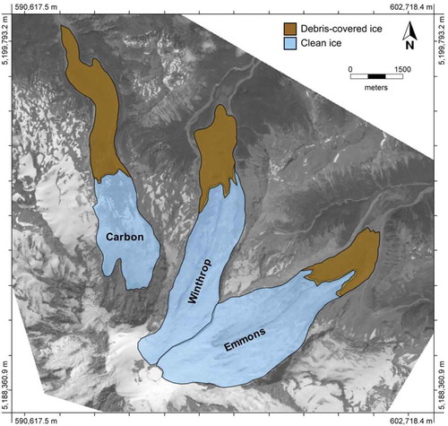
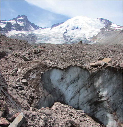
Figure 2. View across the debris-covered terminus of Emmons Glacier toward the summit of Mount Rainier (right) and Little Tahoma (left). Field measurements in 2014 took place just beyond the triangle-shaped boulder rising above the debris-covered ice in the middle ground.

Despite these similarities, Emmons, Winthrop, and Carbon glaciers differed in their response to late twentieth- and early twenty-first-century climate changes. From 1970 to 2008, Carbon Glacier lost $97.9\times {10}^6$ m³ of ice, mostly by terminus thinning, while Winthrop Glacier lost $24.3\times {10}^6$ m³ by thinning, despite modest thickening at the toe. Over the same period, Emmons Glacier added $13.8\times {10}^6$ m³ of ice marked by a slight terminal advance and thickening (Sisson, Robinson, and Swinney 2011). These differences may be attributed to some combination of topographic and microclimatic settings and differences in supraglacial debris distribution. Which of these factors accounts for most of the differences remains unknown. This study is aimed in part at evaluating whether differences in supraglacial debris distribution could explain some of the divergent mass balance trends.

Background

Supraglacial debris has a complex effect on ablation that causes debris-covered glaciers to interact with the atmosphere differently than debris-free glaciers (Anderson and Anderson, 2016; Nakawo and Young 1981; Nicholson and Benn 2013; Østrem 1959; Scherler, Bookhagen, and Strecker 2011). In alpine settings where many debris-covered glaciers are located, predicting the local response to climate change and glacial contributions to the water resources is of critical importance for water resource planning and hazard mitigation, among other things. As a result, the impacts of debris on energy budgets and mass balance have received increasing attention from geoscientists (e.g., Nicholson and Benn 2013; Reznichenko, Davies, and Alexander 2011; Richardson and Reynolds 2000; Scherler, Bookhagen, and Strecker 2011; Thompson et al. 2016).

A glacier’s response to supraglacial debris is sensitive to the debris thickness and spatial distribution, which vary according to debris sources and are subsequently affected by various transport processes at the glacier surface (Moore 2018). Moore (2018) showed that supraglacial debris could be destabilized not only on oversteepened slopes, but also where the ratio of ablation rate to debris hydraulic conductivity is large. Mapping of potential instability on the debris-covered margin of Emmons Glacier identified extensive areas that could be prone to debris destabilization and local gravitational transport (Moore 2018). Debris thicknesses can thus vary greatly over distances as little as a few meters, making the spatial pattern of mass balance on debris-covered glaciers highly complex (Nicholson et al. 2018). This poses a challenge for the study of debris impacts, as the local variability makes representative field-based study time- and resource-intensive, while conventional remote-sensing methods lack the spatial resolution needed to capture local variability. Developing technologies in high-resolution imaging from unmanned aircraft have the potential to foster great advances in the near future (e.g., Kraaijenbrink et al. 2018), but in the meantime, combined field and remote-sensing studies hold the most promise for understanding debris effects.

A functional relationship between debris thickness and ablation rates was established several decades ago (Østrem 1959) and has been corroborated in subsequent studies (e.g., Collier et al. 2015; Juen et al. 2014; Mihalcea et al. 2006; Nakawo and Young 1981; Takeuchi, Kayastha, and Nakawo 2000). Thin debris cover (less than a few centimeters) yields melt rates greater than those of clean ice due to the increased absorption of incoming shortwave radiation. However, a thicker debris cover greatly decreases ablation as the conductive thickness of the debris grows and greater fractions of received radiation are returned to the atmosphere. In principle, debris cover greater than a meter or two could make ablation negligible, although at this point other processes could contribute substantially to mass loss, including ice-cliff backwasting and migration of supraglacial ponds (Krüger and Kjær 2000; Brun et al. 2016; Miles et al. 2016).

If supraglacial debris is present in sufficient thickness on a significant portion of a glacier’s ablation zone, mass loss by surface ablation can be greatly suppressed, slowing terminal retreat under a warming climate (Scherler, Bookhagen, and Strecker 2011; Basnett, Kulkarni, and Bolch 2013; Dobhal, Mehta, and Srivastava 2013; Brun et al. 2016). In extreme cases, substantial supraglacial debris cover has been thought to promote anomalous terminus advance or thickening (Vacco, Alley, and Pollard 2010; Reznichenko, Davies, and Alexander 2011). Alternatively, some glaciers with extensive supraglacial debris maintain rates of mass loss comparable to debris-free ice, indicating that processes beyond simple downwasting could be important in governing debris-covered glacier balance in some settings (Gardelle, Berthier, and Arnaud 2012; Banerjee 2017). Thus, the presence and extent of debris cover make up only one of many variables that can impact the mass balance pattern of a glacier in time and space.

The dominant heat transfer processes that govern ablation of debris-covered glaciers scale directly or indirectly with the debris surface temperature (e.g., Nicholson and Benn 2006). Many researchers have included point measurements of debris surface temperature (e.g., Fyffe et al. 2014), but large spatial and temporal variations make it challenging to extrapolate surface temperature across and among glaciers. Fortunately, surface temperature can be retrieved from many modern satellite products, and various methods have been developed for combining satellite and in situ field measurements to permit spatially distributed modeling for ablation studies (Mihalcea et al. 2008; Zhang et al. 2011; Foster et al. 2012; Fyffe et al. 2014). The spatial resolution of most widely available satellite thermal imagery is limited by the pixel size of the image (typically 60 m on a side), and therefore cannot capture the small-scale variability in debris thickness and debris surface temperature. Nevertheless, this technology allows glacier researchers to identify spatial variations in debris properties in a way that is not practical in field studies.

Various aspects of the debris covered glaciers of Mount Rainier have been studied in the past. Burbank analyzed moraines to reconstruct the Holocene and twentieth-century mass balance and terminus fluctuations of several glaciers on Mount Rainier, including Carbon and Winthrop glaciers (Burbank 1981, 1982). Nylen (2004) analyzed historical aerial photos and digitized past extent of all of Rainier’s glaciers. More recently Rasmussen and Wenger (2009) estimated mass balance parameters for Emmons Glacier using atmospheric remote sensing methods, and Sisson, Robinson, and Swinney (2011) compared 2007/2008 LiDAR elevations with re-projected 1970 U.S. Geological Survey (USGS) topography to estimate ice volume change in the intervening period. Fountain and others mapped the current and historic extent of Carbon, Winthrop, and Emmons glaciers as part of the GLIMS program (Fountain et al. 2014). The National Park Service has maintained Emmons Glacier as a study site, periodically releasing public information on its mass balance (Riedel and Larrabee 2011, 2015). Park staff also continue to update maps of glacier and debris-cover extent, motivated in part by concern over debris-related hazards and impacts on park infrastructure (Beason 2017).

Debris properties and distribution have received less attention on Rainier’s glaciers, but some studies provide useful insights. Crandell and Fahnestock (1965) described the properties and extent of debris covering Emmons Glacier following the 1963 rockfall event. Mills described textural properties of several facies of glacial sediments on Mount Rainier, including supraglacial debris from each of our study glaciers (Mills 1978). Fickert, Friend, and Grüninger (2007) studied the microclimate and vascular plant assemblage atop and within the debris cover of Carbon Glacier, where they documented debris surface temperature and thickness. None of these studies has sought to reveal the impact of debris cover properties and distribution on observed and projected glacier extent and mass balance. However, the correlation in time between the 1963 Little Tahoma rockfall and the advance of Emmons Glacier has been noted by several authors (Beason 2017).

Methods

Field measurements

We conducted field measurements of debris properties and subdebris ablation in a small field site (60 m by 60 m) near the centerline of Emmons Glacier, at an elevation of approximately 1500 m. From 31 July to 10 August 2014, a grid of 16 ablation stakes (polyvinyl chloride [PVC] or crosslinked polyethylene [PEX]) was installed in the ice beneath the debris in this area using a Kovacs hand drill. The site was chosen to span several debris types (ranging from open-work boulders to well-sorted sand to sandy diamict) and thicknesses varying from a few centimeters to more than 0.5 m (Table 1). Debris texture and moisture content were noted at each stake site during installation. At each ablation stake, local slope and aspect were measured with a Brunton compass.

Table 1. Debris properties and observations at ablation stake sites, Emmons Glacier, August 2014.

Stake	$H$ (cm)	$\dot{m}$ (mm/d)	$\overline{T_s}$ (°C)	Site description
A1	21.5	26.6	19.0	Small boulders, large cobbles, gravel and sand
A2	11.5	26.9	16.4	Small cobbles and pebbles; moist gravel and sand at depth
A3	31	18.1	18.3	Large cobbles, gravel and sand
A4	44	19.4	17.9	Small boulders, large cobbles, gravel and sand
B1	12	30.5	13.2	Moist sand with pebbles and small cobbles
B2	24	26	17.4	Boulders and cobbles; uneven ice surface
B3	20	25.5	18.3	Large cobbles, moist sand and gravel
B4	22.5	13	16.3	Large cobbles and moist sand and gravel
C1	9	32.3	11.7	Small boulders, gravel and sand; site is partly shaded
C2	3	38.7	12.3	Boulders, small cobbles, gravel and sand
C3	10	27.7	14.0	Moist sand and gravel
C4	5.5	32.1	12.8	Large cobbles, moist gravel and sand; site shaded by boulder
D1	31	20.3	20.3	Small boulders and large cobbles, no matrix
D2	18	7.1	14.3	Small cobbles and moist gravel
D3	26.5	27.8	18.5	Small boulders, gravel and moist sand; fully saturated
D4	10	32.3	13.8	Cobbles and moist gravel

Ablation rates were determined by measuring the exposed height of each stake during early afternoon on alternate days. Debris surface temperature around each stake was measured with a hand-held noncontact infrared thermometer (Control Company Traceable MiniiiIR), and changes in the debris texture and weather conditions were noted. Additionally, Hobo pendant temperature loggers (Onset) were set on top of and within debris of varying thickness to measure debris temperature automatically at 15-minute intervals throughout the study period. Several thermistors (Honeywell 5 kΩ NTC) were placed on the debris surface or within debris near the Hobos to verify temperatures.

Meteorological data was recorded by an automated weather station (AWS) erected in the center of the field site. The AWS was equipped with a Campbell Scientific CR 1000 datalogger, a Campbell Scientific 107-L radiation-shielded temperature probe to measure 2-m air temperature, and a Huskeflux LP02 pyranometer with a 285- to 3000-nm waveband to measure incoming shortwave radiation. The AWS was powered by a gel-cell battery trickle charged with a 5-W solar panel. Air temperature and incoming shortwave radiation were recorded for the entire study period at 15-minute intervals.

Mean ablation rates measured over the full study period were used to estimate the effective thermal conductivity $K$ of the debris using a linear approximation to the heat conduction equation. Assuming that all heat used for melting conducted through the debris and is proportional to the mean daily surface temperature at each stake site, ablation rate $\dot{m}$ can be estimated as:

(1) $\dot{m}=\frac{\overline{T_s}K}{\rho LH}$(1)

where $\rho$ is the density of ice, $L$ is the latent heat of fusion, $H$ is debris thickness, and $\overline{T_s}$ is the daily mean debris surface temperature (Nakawo and Young 1981; Nicholson and Benn 2006). This formulation is a simplification of the linear heat conduction equation that takes advantage of the fact that the temperature gradient $\left(T_s-T_i\right)/H$ can be simplified to $T_s/H$ when the ice is at its melting temperature expressed in °C. Equation 1 can be rearranged to solve for $K$ when surface temperature, debris thickness, and ablation rate are measured directly. This approach has been used in the past to show that effective $K$ values vary with thickness, perhaps due in part to differences in thermal properties of different materials or different heat transfer processes (e.g., ventilation of open-work cobbles) transporting heat through the debris (Brock et al. 2010).

Remote sensing

A single Landsat 8 scene covering Mount Rainier and its surroundings was captured on 7 August 2014, coinciding with part of our field campaign on Emmons Glacier. This imagery was processed both to estimate the extent of clean and debris-covered ice and to retrieve land-surface temperature. Temperature was retrieved from thermal infrared Band 10 by conversion of image DN values to top-of-atmosphere radiance and subsequently to brightness temperature using recommended methods from the U.S. Geological Survey. An enhanced single-channel algorithm with atmospheric corrections was then used to determine land-surface temperature (Wang et al. 2016).

The ice margin was digitized from aerial photos and from the panchromatic band (Band 8) from the same Landsat scene. The approximate extent of continuous debris-covered ice was digitized manually but guided by a combination of thermal imagery and a k-means (k = 3: snow, ice, rock) image classification of the raster computed from band ratio panchromatic/short-wave infrared (SWIR) (B8/B6) (Paul et al. 2016). For this application, pixels with average temperatures less than or equal to the ice melting temperature were excluded, and this necessarily eliminated some areas of very thin or patchy debris cover. Thus, debris-covered areas and volumes derived from this approach should be considered minima.

Distributed energy balance

We describe the energy balance at the surface of a debris-covered glacier using the point model of Foster et al. (2012):

(2) $Q_s+Q_l+Q_h+Q_e-Q_c=0$(2)

where $Q_s$ is the net shortwave radiation (defined as incoming solar radiation minus the reflected solar radiation), $Q_l$ is the net long-wave radiation, $Q_h$ is the turbulent sensible heat flux, $Q_e$ is the evaporative heat exchange, and $Q_c$ is the conductive heat flux (upward or downward) through the debris. All terms are expressed in $\mathrm{W}/{\mathrm{m}}^2$ and averaged over 1 day.

For remote-sensing applications, some of the energy-balance terms in Equation 2 that cannot be measured directly can be omitted or parameterized when conditions on the ground permit. One important challenge, however, is that the surface temperatures retrieved from satellite imagery do not necessarily represent mean daily values. Debris-surface temperatures higher or lower than the local daily average reflect transient heating and cooling in response to the diurnal radiation cycle, producing nonlinear temperature profiles through supraglacial debris at the time of satellite image acquisition. These transients indicate changes in the heat stored within the debris and can be treated as a separate energy balance term. Brock et al. (2010) called this term $\mathrm{\Delta }D$ and, following Mattson and Gardner (1989), estimated its value by measuring the rate of change of the mean debris temperature within a debris mass. The rate of temperature change $d{T}_m/dt$ multiplied by the bulk density $\rho$, specific heat capacity $C_d$, and thickness $H$ of the debris yields an energy flux into or out of storage in the debris (Mattson and Gardner 1989). The approach of Brock et al. (2010) assumes that the mean debris temperature at any place and time is the average of the debris surface temperature and the temperature of the ice surface beneath. Foster et al. (2012) reasoned that because $\mathrm{\Delta }D$ represents the difference between heat conducted into the debris mass and the heat used for melting, it could be scaled with $Q_c$. These authors accordingly expressed the transient heat storage term $\mathrm{\Delta }D=-F{Q}_c$ (Foster et al. 2012, 680).

Thus, the energy balance can be modified to include a term $\left(1+F\right)$ multiplying the conductive heat flux, where $F$ is a dimensionless empirical constant that accounts for storage (Foster et al. 2012). $F$ is estimated here from debris-surface temperature measurements over a several-hour period surrounding satellite image acquisition following the method of Brock et al. (2010).

Evaporative heat transfer $Q_e$ is often assumed to be small on dry debris surfaces and may be safely neglected (Brock et al. 2010). Turbulent sensible heat flux $Q_h$ is difficult to measure directly, and estimates are notoriously sensitive to a scale parameter that constrains the vertical distribution of wind speed (Quincey et al. 2017). Turbulent heat transfer is, however, negligible when wind velocity is low and the temperature difference between the debris surface and the near-surface air is small. These conditions were met during the Landsat 8 OLI scene capture time on 7 August 2014. Therefore, we simplify the energy balance to include only radiation and conduction terms:

(3) $Q_s+Q_l-\left(1+F\right)Q_c=0.$(3)

Net shortwave flux ($Q_s=Q_{s0}\left(1-\alpha \right)$, where $Q_{s0}$ is incoming shortwave radiation and $\alpha$ is the surface albedo) can be measured directly or estimated from models and remotely sensed imagery under clear-sky conditions. The net longwave flux is normally given as

(4) $Q_l={\epsilon }_a\sigma T_a^4-{\epsilon }_s\sigma T_s^4,$(4)

where $\epsilon$ is emissivity, $\sigma$ is Boltzmann’s constant, $T$ is temperature, and the subscripts $a$ and $s$ refer to properties of air (commonly at 2 m above the surface; Hock 2005) and the debris surface, respectively. While $T_s$ is inherently spatially distributed when retrieved from satellite thermal imagery, it is more difficult to efficiently measure spatial variation in $T_a$ at the same time. Indeed, the distribution of air temperature over debris-covered glaciers has not been found to correlate well with altitude in a simple way. Rather, near-surface air temperature correlates better with debris surface temperature during the daytime (Steiner and Pellicciotti 2016). Here, we follow the method outlined in Foster et al. (2012) and tested by Steiner and Pellicciotti (2016), wherein $T_a$ is expressed as an empirical function of $T_s$ based on linear regression of the two variables measured during late morning. We therefore make a substitution of the form $T_a=c_1{T}_s+c_2$ in Equation 4, based on regression of measured 2-m air temperature and one of the Hobo temperature loggers located at a representative site on the debris surface.

For one-dimensional steady-state conduction, $Q_c$ may be defined as

(5) $Q_c=\frac{T_s}{R}$(5)

where $T_s$ is the debris surface temperature in °C and $R$ is the thermal resistance of the debris. Thermal resistance is defined as $R=H/K$, where $H$ is the thickness of the supraglacial debris and $K$ is its effective thermal conductivity. As mentioned earlier, satellite-retrieved debris surface temperature $T_s$ is not necessarily equal to its daily mean value $\overline{T_s}$ at a given point on the glacier surface.

To identify differences in debris distribution and properties within and among glaciers, Equations 3–5 were combined and solved for $R$, yielding

(6) $R=\frac{\left(1+F\right)T_s}{Q_{s0}\left(1-\alpha \right)+{\epsilon }_a\sigma {\left(c_1{T}_s+c_2\right)}^4-{\epsilon }_s\sigma T_s^4},$(6)

which now depends primarily upon satellite-retrieved debris-surface temperature.

In this analysis, we use the regression for air temperature, measurement of $Q_{s0}$, and the empirically derived value of $F$ determined from field measurements on Emmons Glacier to estimate $R$ for all three glaciers, even though Carbon and Winthrop glaciers have different topographic settings and elevation ranges and perhaps debris properties. The assumption that these variables ($c_1,c_2,Q_{s0},F$) are the same across all three glaciers is a potential limitation of this analysis, and its impact is addressed further in the Discussion section.

The area and distribution of $R$ values on each glacier were further used to estimate debris thickness and total debris volume for comparison among glaciers. Equation 1 was used with ablation stake measurements to estimate $K$. A best-fit function was then determined for $K$ as a function of $H$ and substituted for $K$ in the definition of thermal resistance, $R=H/K$. The resulting formula was used to estimate the mean debris thickness in each pixel in the $R$ rasters.

Results

Debris in our study area varied from boulder fields exceeding 0.5 m thick to isolated, steeply sloping ice cliffs maintained debris-free by mass wasting. Debris properties and descriptions are given in Table 1. The mean thickness measured during ablation stake installation (n = 16) was 18.7 cm. Textures ranged from boulders to silty sand and gravel. In debris cover containing material finer than gravel, there was some concentration of these fines toward the bottom of the profile. Debris was often moist up to a height of around 10 cm from the debris–ice interface at each site with gravel and finer material. Where the debris thickness was 10 cm or less, the debris surface was moist. Ablation stakes were installed in ice with debris cover ranging from 3 to 44 cm thickness and including much of the textural range observed.

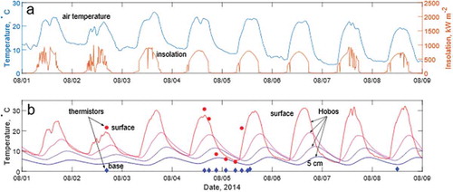
Weather conditions during the study period were calm and warm, with mostly clear skies and daytime highs near 20°C (Figure 3a). Conditions at the time of Landsat image acquisition on August 7 were clear and calm, with air temperature approximately 14°C at the Emmons Glacier field site. Debris temperature as measured with thermistors, infrared sensors, and Hobos was very warm during the daytime, with surface temperature reaching in excess of 30°C in areas of thick debris. Areas with thinner or wetter debris tended to be cooler (Table 1). Temperature fluctuations with depth at one site with 0.5-m-thick debris were consistent with conductive heat transfer from the debris surface to the ice (Figure 3b).

Figure 3. Data from the temporary meteorological station and wireless temperature sensors installed on Emmons Glacier during early August 2014. (a) Air temperature 2 m above the glacier surface (left axis) and incoming shortwave radiation (right axis). (b) Debris temperature measured by thermistors (points) and Hobo pendant loggers (lines) at uniform depth intervals throughout a 0.5-m debris layer.

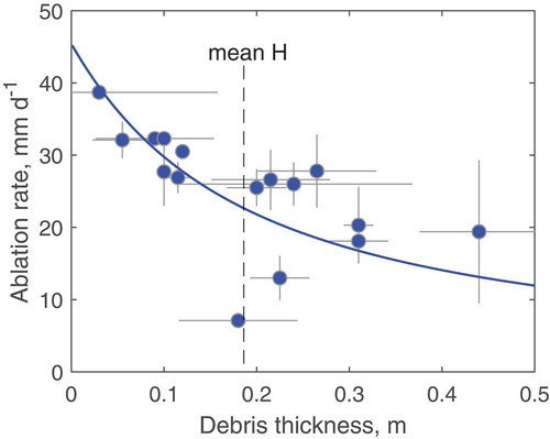
Ablation rates in the study area ranged from 39 mm/d beneath the thinnest debris cover to as low as 7 mm/d beneath thicker debris (Figure 4). While many studies have shown strongly developed exponential or geometric decay in ablation rates with increasing debris thickness, our data show substantial scatter. This may reflect a broader range of topographic and textural properties of the debris-covered surfaces we measured or alternatively some artifact of the small data set and the short study duration. Even so, there is a general trend of decreasing ablation rates beneath increasing debris thickness. The stake data are shown in Figure 4 along with a solution to Equation 2 following an energy-balance method modified from Nicholson and Benn (2006) and with parameter values given in Table 2.

Table 2. Values of variables and constants used in simplified energy balance model (Equation 2) and satellite retrieval of thermal resistance (Equation 6).

Variable, units	Value
$Q_{s0}$, W m^−2	231 (Equation 2); 470 (Equation 6)
$T_a$, K	288 (Equation 2)
$\alpha$, dimensionless	0.3
$F$, dimensionless	0.71
$\sigma$, W m^−2 K^−4	5.39 $\times$ 10^−8
${\epsilon }_a$, dimensionless	0.7 (Hock 2005)
${\epsilon }_r$, dimensionless	0.95
$c_1$, dimensionless	0.384
$c_2$, °C	11.5

Figure 4. Ablation rate, averaged over 8 days of measurement, plotted as a function of debris thickness. Dots are field measurements, while the line represents a numerical solution of the energy balance model of Nicholson and Benn (2006) driven with averaged in situ measurements of solar radiation and estimated thermal conductivity from the Emmons Glacier field site over the measurement interval. Horizontal error bars represent uncertainty in debris thickness determination, estimated as 0.25 times the largest particle diameter adjacent to the stake. Vertical error bars represent one standard deviation of the daily variation in melt rate at each stake.

Thermal conductivity estimated from Equation 1 with measured surface temperature, debris thickness, and ablation rate ranged from 0.33 to 1.66 W m⁻¹ °C⁻¹, with a mean value of 0.89 W m⁻¹ °C⁻¹. With the exception of the lowest values, these estimates of $K$ are within the range of values determined elsewhere (e.g., Nicholson and Benn 2006), and variations likely reflect differences in texture and moisture. Similar to Brock et al. (2010), we note an apparent increase in effective conductivity with increasing debris thickness. The data are best fit with the power function $K=1.98H^{0.48}$, although with a weak coefficient of determination ($r^2=0.5)$, suggesting that one or more variables unrelated to debris thickness also strongly govern effective conductivity.

Land surface temperature for the region during late morning of 7 August 2014 varies from below freezing to nearly 40°C on south-facing rock slopes beyond the ice margin. The warmest areas of debris-covered glacier are near the northern ice margin of Emmons Glacier, reaching about 28°C. Air temperatures computed from the empirical relationship described earlier ranged from 10°C to 23°C. The air temperature computed in this manner at the site of our direct temperature measurement is about 19°C, significantly higher than 14.1°C measured directly on site. This difference most likely reflects the fact that the regression used to relate $T_a$ and $T_s$ included data from earlier in the study period when late-morning air temperatures were much warmer.

Estimated areas of each glacier and their debris-covered portions are shown in Table 3 (see also Figure 1). Glacier areas are within 3% of those reported for 2015 in the National Park Service’s glacier inventory of Mount Rainier by Beason (2017). However, because we limited our debris delineations to contiguous areas with surface temperature greater than the ice melting temperature (273.15 K), debris-covered areas are significantly smaller in this estimate than in the National Park Service report (Beason 2017).

Table 3. Size and estimated debris extent of study glaciers from remote-sensing analysis.

Glacier	Total area (m^2)	Debris area (m^2)	Debris volume (m^3)	Percent covered	Mean debris H (cm)
Carbon	7,450,732	3,167,698	182,289	43%	5.6
Emmons	11,230,885	1,921,975	177,847	17%	9.0
Winthrop	8,763,390	2,218,931	191,272	25%	8.2

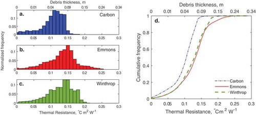
Figure 5 shows thermal resistance $R$ computed with Equation 6 for each debris-covered terminus. Table 2 gives constants and parameter values used in this computation. The color scale in Figure 5 remains fixed for all three glaciers, highlighting the presence of larger $R$ values across Emmons and Winthrop glaciers compared with Carbon Glacier. Mean values of $R$ estimated for Carbon, Emmons, and Winthrop glaciers are 0.105, 0.136, and 0.132°C m² W⁻¹, respectively. Frequency distributions and cumulative frequency curves for $R$ values for each glacier are shown in Figure 6. Note that more than 90% of the debris-covered area of Carbon Glacier has $R$ values less than the mean values for the other two glaciers (Figure 6d). The distributions for Emmons and Winthrop glaciers, however, are very similar.

Figure 5. Estimated thermal resistance [°C m² W⁻¹] of the Carbon, Winthrop, and Emmons (from upper left to lower right) debris-covered termini, overlain on a hillshade map. The color scale remains fixed over all three termini, and warmer colors indicate higher thermal resistance.

Figure 6. Normalized discrete (a–c) and cumulative (d) frequency distributions of thermal resistance on each debris-covered glacier terminus. Equivalent debris thickness, according to the best fit function given in the main text, is shown as an upper (nonlinear) horizontal axis for reference. The colors in the bar charts (a–c) match the color of the corresponding cumulative frequency curve (d).

Discussion

As expected from prior work on debris-covered glaciers, thicker debris on Emmons Glacier generally suppressed ablation more than thin debris. The substantial scatter around the general trend seen in Figure 4 could be caused by a number of variables. Because we made no effort to select ablation stake sites in uniformly textured debris, some of the scatter could be due to real differences in optical or thermal properties of different types of debris. Alternatively, it could reflect processes transporting heat to or from the debris surface that are not uniform across all stakes. Processes like convection and evaporation potentially affected some stake sites more than others due to ice-surface topography or debris texture variations. Indeed, our debris-surface temperature measurements made during measurements of ablation stakes do indicate that the stakes lying farthest below the model curve in Figure 4 had unusually low debris surface temperatures. Regardless of the cause of scatter, we observe a weaker development of the typical Östrem curve, but one that nevertheless captures the expected trend.

The key variable linking our field measurements to satellite measurements is thermal resistance, $R$. Since $R$ is not directly measured in the field, we must relate it to debris thickness through effective thermal conductivity, $K$. Estimates of $K$ from ablation stake measurements vary by a factor of 5, and, as discussed earlier, this could result from the implicit inclusion of nonconductive heat transfer in computing $K$. If $K$ were in reality 50% larger or smaller, this would primarily affect the transfer function $H=KR$ used to retrieve debris thickness from $R$ rasters. Recall, for example, that our measured debris thicknesses in the study area averaged approximately 18 cm or 0.18 m. Taking $K$ = 0.89 W m⁻¹ °C⁻¹ as a first estimate of conductivity and multiplying the $R$ value in the pixel closest to the study site (0.151°C m² W⁻¹) indicates that model-estimated debris thickness there would be 0.134 m. If we set $K$ = 1.20 W m⁻¹ °C⁻¹ instead (a 35% increase), the predicted debris thickness would match closely our measured thicknesses. However, there is no other basis for making this adjustment and assuming that $K$ is the cause of inconsistency between direct field measurements and satellite estimates of $H$. This example illustrates the sensitivity of these results to a key, imperfectly constrained effective $K$ that likely varies both in space and time.

Assuming that our measurements and functional representation of $K$ are valid across Emmons Glacier and do not systematically vary among glaciers, we may derive debris thickness and volume rasters across the debris-covered termini. Combining the empirical relationship between $K$ and $H$ with the definition of $R$ gives the formula $H=3.72R^{1.92}$. Thickness estimates (pixel averages) across the three glaciers range from zero to approximately 34 cm, with the largest values along the northern margin of Emmons Glacier. Multiplying mean pixel depth by pixel area and summing over each glacier provides a minimum (because of the expected underestimate of debris area) debris volume for each glacier. Surprisingly, this volume estimate is similar for all three glaciers, averaging around 184,000 m³ of debris. The authors are not aware of any other estimates of the current debris volume with which to compare these values. However, Crandell and Fahnestock (1965) estimated that “several million cubic yards” (1 yd³ = 0.765 m³) of rock debris covered an area of about 1.3 square miles (~3,367,000 m²) of Emmons Glacier following the 1963 rock avalanche from Little Tahoma Peak (Crandell and Fahnestock 1965, A18). While we estimate an area of debris cover on Emmons Glacier of just more than half of this, our volume estimate is almost an order of magnitude smaller than a conservative interpretation of Crandell and Fahnestock’s volume (2 million cubic yards ~ 1,530,000 m³) and is two orders of magnitude smaller than the volume estimated from a seismological analysis of the event (11,000,000 m³ [Norris 1994]). These published estimates include rockfall material that was deposited beyond the ice margin. In addition, glacier motion and ablation should have transported a portion of the debris to the terminus to be deposited in moraine or reworked by meltwater. Glacier flow velocity measurements by Allstadt et al. (2015) indicate that Emmons Glacier moves as fast as 1.5 m/d near the equilibrium line and less than 0.05 m/d in the debris-covered margin. If this range of short-term velocities is representative of Emmons Glacier over the 51-year period from 1963 to 2014, passive transport of material from mid-glacier to the terminus (currently a distance of ~3000 m) would have taken anywhere from 5 to 165 years. This suggests that some of the Little Tahoma debris that was deposited on Emmons Glacier in 1963 is likely beyond the ice margin, accounting for at least some of the discrepancy between our estimates and those of earlier studies. Since no major terminal moraine with debris volume of order 10⁶ m³ is present at or near the current ice margin, most of the debris released at the terminus has likely been moved by meltwater farther downstream through the White River drainage. Some Little Tahoma debris still remains atop the glacier, however, particularly near the southern edge of the terminus where ice motion is likely on the lower end of the range measured by Allstadt et al. (2015).

Extrapolation of debris properties and ablation trends from a field study site to larger areas requires knowledge of several other spatially variable quantities that are not well known. In particular, the near-surface (2-m) air temperature is important in the energy exchange between the atmosphere and the debris surface. As we have only one reliable measurement of air temperature over the debris-covered ice, obtaining spatially distributed temperature measurements requires parameterizing air temperature with another quantity for which we have spatially resolved information, such as elevation or surface temperature. Our analysis here has used a method discussed in the literature that assumes that daytime debris surface temperature is a better predictor of air temperature than elevation on a given valley glacier (Steiner and Pellicciotti 2016). However, we have made the further assumption that this relationship can be extended across adjacent valleys as well. If air temperature were adjusted to account for differences in air masses or elevations amounting to a few degrees of offset, the predicted longwave balance would increase (warm the debris surface) by around 3.6 W m⁻² per 1°C increase in air temperature, which would have only a minor impact (1.3% per 1°C) on computed thermal resistance.

A more significant source of uncertainty is the $F$ term introduced in the analysis of transient heat storage in the debris on time scales of minutes to hours. This numerical term was proposed to eliminate the need to measure subsurface debris temperature to account for changes in heat storage within debris. Following Foster et al. (2012), we estimated $F=0.71$ based on the average change in mean debris temperature over a 2-hour window surrounding satellite scene acquisition (following Brock et al. 2010, Equation 7). This value was determined using a temperature logger resting on 15-cm-thick debris, which is close to the average debris thickness at the study site. However, performing the same analysis with a second temperature logger on 49-cm-thick debris yielded $F=7.2$. This number probably overestimates energy storage in the debris, as the vertical temperature gradient during late morning heating is likely not linear for debris this thick.

Schauwecker et al. (2015) attempted to correct for some of these problems with the Foster approach by assuming that transient heat storage within debris involves a fraction (usually 0.5) of the full debris thickness, allowing for limited profile nonlinearity. They also used data from prior work to show that $F$ varies systematically with debris thickness, and described a method for iteratively solving for $F$ and $H$. However, their limited data suggested that $F$ varied minimally for debris thinner than 40 cm. Rounce and Mckinney (2014) used a similar approach to approximate the nonlinear nature of heat storage, yielding acceptable results but with the same limitations. Clearly, more data are needed to improve confidence in these parameterizations of stored heat.

Because we generally cannot retrieve in any satellite thermal image the mean daily debris surface temperature at every point on a debris-covered glacier, the use of daily-mean energy balance methods to retrieve debris properties and distribution requires care. A robust method for assessing either the transient debris heat storage or the departure of measured temperature from the daily mean is essential. More data on subsurface debris temperatures with high temporal resolution would be valuable in developing this foundation. In addition, physical modeling of heat transfer within a debris layer aimed at testing the assumptions of Brock et al. (2010) and Foster et al. (2012) would be valuable.

Many of these limitations and approximations affect estimates of all three of the debris-covered termini in this study in a similar way, provided that the assumptions are no worse on one glacier than on another. Consequently, while they affect the particular numerical results for debris thicknesses and volumes, the differences between glaciers are less sensitive to these limitations. Even if we are cautious with interpreting the $R$, $H$, or $V$ numerical values, comparisons across glaciers should remain robust. Therefore, the finding that Carbon Glacier’s debris cover has a significantly smaller mean and median $R$ value would likely not change with reasonable parameter adjustments.

Implications for mass balance

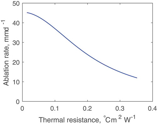
The extrapolated distributions of thermal resistance have important implications for the mass balance of the large debris-covered glaciers of Mount Rainier. Increasing thermal resistance leads to a reduction in melt rate for a given set of meteorological conditions, at least for debris thicknesses greater than a few centimeters. Figure 7 shows hypothetical ablation rates as a function of thermal resistance for meteorological conditions like those observed at Emmons Glacier during our field study. This curve was generated with daily mean values measured on the Emmons terminus during early August, including a functional representation of the dependence of $K$ on $R$. This curve (and our dataset) does not include an ablation rate for bare ice, but two different sources suggest that a degree-day factor for bare ice on Emmons Glacier could lie between 6 and 7 mm °C⁻¹ d⁻¹ (Rasmussen and Wenger 2009; Riedel and Larrabee 2011). If the daily mean air temperature during the same period is between 5 and 10°C over bare ice, we would expect bare-ice ablation to fall in the range 30–70 mm d⁻¹. Assuming that 45 mm d⁻¹ is therefore a reasonable point of comparison for bare ice with no thermal resistance during the same period, we would predict a reduction in melt by around 20% where $R$ averages 0.105°C m² W⁻¹ ($H=0.043$ m) and almost 30% where $R$ averages 0.136°C m² W⁻¹ ($H=0.072$ m). These figures represent averages for Carbon and Emmons glaciers, respectively, and illustrate how significant the difference in mass balance can be with relatively small differences in debris thermal resistance and hence debris thickness across glaciers.

Figure 7. Modeled relationship between thermal resistance and daily ablation rate for average weather conditions observed on Emmons Glacier during 1–10 August 2014, including the apparent increase in effective thermal conductivity on thermal resistance.

We return now to the broader question of whether debris cover differences can partially explain the divergence in apparent glacier health across the last decades of the twentieth and early twenty-first centuries. We are reasonably confident that although all three glaciers in the study have similar debris volumes, the debris is spread on average in a thinner blanket on Carbon Glacier than the other two. Thus, despite the greater debris-covered area, a given square meter of Carbon Glacier’s surface has less debris to attenuate ablation.

The differences in behavior between Winthrop and Emmons glaciers are not as clearly related to the current debris cover, as $R$ distributions are very similar between the two glaciers. A likely culprit for the difference in behavior is the abrupt change in 1963 in the extent of debris cover on Emmons Glacier, which had a smaller area than Carbon Glacier at the beginning of the twentieth century (Nylen 2004). The rapid increase in thermal resistance over a large fraction of a glacier that previously had adjusted its volume and extent to less extensive debris cover would be expected to cause a transient increase in ice volume and terminus extent. Indeed, deposition of extensive rockfall debris is thought to have caused Franz Josef Glacier in New Zealand to undergo anomalous advance several kilometers downvalley and deposit the distinct Waiho Loop moraine (Vacco, Alley, and Pollard 2010; Reznichenko, Davies, and Alexander 2011). It is likely that the post-1963 advance and thickening of Emmons Glacier’s terminus have been in part an adjustment to the Little Tahoma rockfall. If this is the case, the adjustment of Emmons Glacier is tied to the persistence of the rockfall debris on the terminus. If the discrepancy between our estimate of Emmons Glacier’s 2014 supraglacial debris volume and the volume thought to have been present shortly after 1963 is real, this implies that a large fraction of the Little Tahoma rockfall debris has been moved to and beyond the ice margin, and no longer affects Emmons Glacier’s mass balance.

An alternative hypothesis for the different behaviors of the debris-covered ice margins is that basin-scale accumulation or ablation regimes differ significantly among glaciers. Observations of volume change between 1970 and 2007/2008 across Mount Rainier as a whole indicated that glaciers with easterly aspects (particularly Emmons and neighboring high-elevation Fryingpan Glacier) grew modestly over that period while most other glaciers lost volume (Sisson, Robinson, and Swinney 2011). Because Fryingpan Glacier lacks significant debris cover, this argues for some spatial variation in another mass balance variable independent of debris cover. Differences in slope and aspect among glaciers may also account for some difference in solar energy available for debris warming. However, solar radiation modeling by Nylen (2004) suggests that midsummer insolation at the three glaciers differs by less than 10%. Moreover, Emmons Glacier is modeled to receive the most solar energy of the three while Winthrop Glacier receives the least. This therefore could not explain both Emmons and Winthrop glaciers’ more positive mass balance.

Conclusions

Field measurements and remotely sensed thermal image analysis were combined to investigate the impact of supraglacial debris on the ablation of three adjacent glaciers on the north and east slopes of Mount Rainier. Our results in the field were consistent with the expectation that the debris cover atop Carbon, Winthrop, and Emmons glaciers suppresses ablation there. However, significantly smaller debris thermal resistance on Carbon Glacier compared to the other two suggest that some of the observed differences in recent ice margin change can be explained by debris thickness or thermal conductivity differences. The more substantial advance and thickening in Emmons Glacier’s terminus compared with Winthrop Glacier cannot be easily explained by systematic differences in debris distribution. Instead, the difference likely reflects the adjustment of Emmons Glacier to vastly increased debris cover following the 1963 Little Tahoma rockfall. A reconstruction of the impact of this event on the mass balance of Emmons Glacier would be a valuable future modeling exercise.

While the numerical results presented here should be considered low-end estimates for thermal resistance, thickness, and volume of debris, the qualitative relationships across glaciers are reliable. Thus, even if the numerical values used, for example, in the retrieval of debris thickness distributions are in error, this should not significantly impact the differences observed between glaciers. With this in mind, we identified air temperature and transient debris heat storage as variables that require further investigation to be used confidently in distributed energy balance modeling. In particular, because the energy delivered to the ice for melting is so sensitive to the transient heat storage term in the energy balance ($\mathrm{\Delta }D$ or $F$), a more thorough theoretical and empirical analysis of this approach is warranted. Advances in measurement or parameterization of these variables will significantly improve the quality and repeatability of satellite-derived supraglacial debris distributions.

Acknowledgments

We thank Andrew Fountain for the use of his Kovacs hand drill, and Justin Ohlschlager, Mariah Radue, and Jayne Pasternak for field assistance. We are grateful to Barbara Samora and Scott Beason for helping to coordinate the logistics of our work at Mount Rainier National Park. This article benefitted from thoughtful reviews by John Andrews and Bob Anderson.

Disclosure statement

No potential conflict of interest was reported by the authors.

Additional information

Funding

This work was supported by NSF-EAR 1225880 to P.L.M., and Carleton College Fund for Environmental Research to L.I.N.

References

- Allstadt, K., D. Shean, A. Campbell, M. Fahnestock, and S. Malone. 2015. Observations of seasonal and diurnal glacier velocities at Mount Rainier, Washington using terrestrial radar interferometry. The Cryosphere 9:2219–35. doi:10.5194/tc-9-2219-2015.
- Anderson, L., and R. Anderson. 2016. Modeling debris-covered glaciers: Response to steady debris deposition. The Cryosphere 10:1105–24. doi:10.5194/tc-10-1105-2016.
- Banerjee, A. 2017. Brief communication: Thinning of debris-covered and debris-free glaciers in a warming climate. The Cryosphere 11:133–38. doi:10.5194/tc-11-133-2017.
- Basnett, S., A. V. Kulkarni, and T. Bolch. 2013. The influence of debris cover and glacial lakes on the recession of glaciers in Sikkim Himalaya, India. Journal of Glaciology 59:1035–46. doi:10.3189/2013JoG12J184.
- Beason, S. 2017. Change in Glacial Extent at Mount Rainier National Park from 1896 to 2015. Natural Resource Report NPS/MORA/NRR-2017/1472, 98.
- Brock, B. W., C. Mihalcea, M. P. Kirkbride, G. Diolaiuti, M. E. J. Cutler, and C. Smiraglia. 2010. Meteorology and surface energy fluxes in the 2005–2007 ablation seasons at the Miage debris-covered glacier, Mont Blanc Massif, Italian Alps. Journal of Geophysical Research 115:D09106. doi:10.1029/2009JD013224.
- Brun, F., P. Buri, E. S. Miles, P. Wagnon, J. Steiner, E. Berthier, P. Kraaijenbrink, W. W. Immerzeel, and F. Pellicciotti. 2016. Quantifying volume loss from ice cliffs on debris-covered glaciers using high-resolution terrestrial and aerial photogrammetry. Journal of Glaciology 62:684–95. doi:10.1017/jog.2016.54.
- Burbank, D. W. 1981. A chronology of late Holocene glacier fluctuations on Mount Rainier, Washington. Arctic and Alpine Research 13:369–86. doi:10.2307/1551049.
- Burbank, D. W. 1982. Correlations of climate, mass balances, and glacial fluctuations at Mount Rainier, Washington, U.S.A., since 1850. Arctic and Alpine Research 14:137–48. doi:10.2307/1551112.
- Collier, E., F. Maussion, L. I. Nicholson, T. Mölg, W. W. Immerzeel, and A. B. G. Bush. 2015. Impact of debris cover on glacier ablation and atmosphere-glacier feedbacks in the Karakoram. The Cryosphere 9:1617–32. doi:10.5194/tc-9-1617-2015.
- Crandell, D. R., and R. K. Fahnestock. 1965. Rockfalls and avalanches from Little Tahoma Peak on Mount Rainier, Washington. In Geological Survey Bulletin 1221-A, 37. Washington, DC: Government Printing Office.
- Dobhal, D. P., M. Mehta, and D. Srivastava. 2013. Influence of debris cover on terminus retreat and mass changes of Chorabari Glacier, Garhwal region, central Himalaya, India. Journal of Glaciology 59:961–71. doi:10.3189/2013JoG12J180.
- Fickert, T., D. Friend, and F. Grüninger. 2007. Did debris-covered glaciers serve as Pleistocene refugia for plants? A new hypothesis derived from observations of recent plant growth on glacier surfaces. Arctic, Antarctic, and Alpine Research 39:245–57. doi:10.1657/1523-0430(2007)39[245:DDGSAP]2.0.CO;2.
- Foster, L. A., B. W. Brock, M. E. J. Cutler, and F. Diotri. 2012. A physically based method for estimating supraglacial debris thickness from thermal band remote-sensing data. Journal of Glaciology 58:677–91. doi:10.3189/2012JoG11J194.
- Fountain, A., H. Basagic, C. Cannon, M. Devisser, M. Hoffman, J. Kargel, G. J. Leonard, K. Thornekroft, and S. Wilson. 2014. Glaciers and perennial snowfields of the US Cordillera. In Global land ice measurements from space, ed. J. Kargel, G. Leonard, M. Bishop, A. Kaab, and B. Raup, 385–408. Berlin: Springer.
- Fyffe, C. L., T. D. Reid, B. W. Brock, M. P. Kirkbride, G. Diolaiuti, C. Smiraglia, and F. Diotri. 2014. A distributed energy-balance melt model of an alpine debris-covered glacier. Journal of Glaciology 60:587–602. doi:10.3189/2014JoG13J148.
- Gardelle, J., E. Berthier, and Y. Arnaud. 2012. Slight mass gain of Karakoram glaciers in the early twenty-first century. Nature Geoscience 5:1–4. doi:10.1038/ngeo1450.
- Hock, R. 2005. Glacier melt: A review of processes and their modelling. Progress in Physical Geography 29:362–91. doi:10.1191/0309133305pp453ra.
- Juen, M., C. Mayer, A. Lambrecht, H. Han, and S. L.-T. Liu. 2014. Impact of varying debris cover thickness on ablation: A case study for Koxkar Glacier in the Tien Shan. The Cryosphere 8:377–86. doi:10.5194/tc-8-377-2014.
- Kraaijenbrink, P., J. Shea, M. Litt, J. Steiner, D. Treichler, and W. W. Immerzeel. 2018. Mapping surface temperatures on a debris-covered glacier with an unmanned aerial vehicle. Frontiers in Earth Science 6. doi:10.3389/feart.2018.00064.
- Krüger, J., and K. H. Kjær. 2000. De-icing progression of ice-cored moraines in a humid, subpolar climate, Kotlujokull, Iceland. Holocene 6:737–47. doi:10.1191/09596830094980.
- Mattson, L. E., and J. S. Gardner. 1989. Energy exchanges and ablation rates on the debris-covered Rakhiot Glacier, Pakistan. Zeitschrift Fur Gletscherkunde Und Glazialgeologie 25:17–32.
- Mihalcea, C., C. Mayer, G. Diolaiuti, C. D. Agata, C. Smiraglia, A. Lambrecht, E. Vuillermoz, and G. Tartari. 2008. Spatial distribution of debris thickness and melting from remote-sensing and meteorological data, at debris-covered Baltoro glacier, Karakoram, Pakistan. Annals of Glaciology 48:49–57. doi:10.3189/172756408784700680.
- Mihalcea, C., C. Mayer, G. Diolaiuti, A. Lambrecht, C. Smiraglia, and G. Tartari. 2006. Ice ablation and meteorological conditions on the debris-covered area of Baltoro glacier, Karakoram, Pakistan. Annals of Glaciology 43:292–300. doi:10.3189/172756406781812104.
- Miles, E., F. Pellicciotti, I. Willis, and J. Steiner. 2016. Refined energy-balance modelling of a supraglacial pond, Langtang Khola, Nepal. Annals of Glaciology 57:29–40. doi:10.3189/2016AoG71A421.
- Mills, H. H. 1978. Some characteristics of glacial sediments of Mount Rainier, Washington. Journal of Sedimentary Research 48:1345–56. doi:10.1306/212F7685-2B24-11D7-8648000102C1865D.
- Moore, P. L. 2018. Stability of supraglacial debris. Earth Surface Processes and Landforms 43:285–97. doi:10.1002/esp.4244.
- Nakawo, M., and G. Young. 1981. Field experiments to determine the effect of a debris layer on ablation of glacier ice. Annals of Glaciology 2:85–91. doi:10.3189/172756481794352432.
- Nicholson, L., and D. I. Benn. 2013. Properties of natural supraglacial debris in relation to modelling sub-debris ice ablation. Earth Surface Processes and Landforms 38:490–501. doi:10.1002/esp.3299.
- Nicholson, L., M. McCarthy, H. Pritchard, and I. Willis. 2018. Supraglacial debris thickness variability: Impact on ablation and relation to terrain properties. The Cryosphere Discussions 1–30. doi:10.5194/tc-2018-83.
- Nicholson, L. I., and D. I. Benn. 2006. Calculating ice melt beneath a debris layer using meteorological data. Journal of Glaciology 52:463–70. doi:10.3189/172756506781828584.
- Norris, R. 1994. Seismicity of rockfalls and avalanches at three Cascade Range volcanoes: Implications for seismic detection of hazardous mass movements. Bulletin of the Seismological Society of America 84:1925–39.
- Nylen, T. H. 2004. Spatial and temporal variations of glaciers (1913-1994) on Mt. Rainier and the relation with climate. M.S. Thesis, Portland State University.
- Østrem, G. 1959. Ice melting under a thin layer of moraine, and the existence of ice cores in moraine ridges. Geografiska Annaler 41:228–30. doi:10.1080/20014422.1959.11907953.
- Paul, F., S. Winsvold, A. Kääb, T. Nagler, and G. Schwaizer. 2016. Glacier remote sensing using Sentinel-2. Part II: Mapping glacier extents and surface facies, and comparison to Landsat 8. Remote Sensing 8:575. doi:10.3390/rs8070575.
- Quincey, D., M. Smith, D. Rounce, A. Ross, O. King, and C. Watson. 2017. Evaluating morphological estimates of the aerodynamic roughness of debris covered glacier ice. Earth Surface Processes and Landforms 42:2541–53. doi:10.1002/esp.4198.
- Rasmussen, L., and J. Wenger. 2009. Upper-air model of summer balance on Mount Rainier, USA. Journal of Glaciology 55:619–24. doi:10.3189/002214309789471012.
- Reznichenko, N. V., T. R. H. Davies, and D. J. Alexander. 2011. Effects of rock avalanches on glacier behaviour and moraine formation. Geomorphology 132:327–38. doi:10.1016/j.geomorph.2011.05.019.
- Richardson, S. D., and J. M. Reynolds. 2000. An overview of glacial hazards in the Himalayas. Quaternary International 65:31–47. doi:10.1016/S1040-6182(99)00035-X.
- Riedel, J. L., and M. A. Larrabee. 2011. Mt. Rainier National Park Glacier Mass Balance Monitoring Annual Report, Water Year 2009. North Coast and Cascades Network, National Park Service. Natural Resource Stewardship and Science, Natural Resource Technical Report NPS/NCCN/NRTR-2011/484, Fort Collins, Colorado.
- Riedel, J., and M. Larrabee. 2015. Mount Rainier National Park Glacier mass balance monitoring annual report, water year 2011 North Coast and Cascades Network Natural resource data series NPS/NCCN/NRDS-2015/752. Fort Collins, CO: National Park Service.
- Rounce, D. R., and D. C. Mckinney. 2014. Debris thickness of glaciers in the Everest area (Nepal Himalaya) derived from satellite imagery using a nonlinear energy balance model. The Cryosphere 8:1317–29. doi:10.5194/tc-8-1317-2014.
- Schauwecker, S., M. Rohrer, C. Huggel, A. Kulkarni, A. Ramanathan, N. Salzmann, M. Stoffel, and B. Brock. 2015. Remotely sensed debris thickness mapping of Bara Shigri Glacier, Indian Himalaya. Journal of Glaciology 61:675–88. doi:10.3189/2015JoG14J102.
- Scherler, D., B. Bookhagen, and M. R. Strecker. 2011. Spatially variable response of Himalayan glaciers to climate change affected by debris cover. Nature Geoscience 4:156–59. doi:10.1038/ngeo1068.
- Sisson, T., J. Robinson, and D. Swinney. 2011. Whole-edifice ice volume change AD 1970 to 2007/2008 at Mount Rainier, Washington, based on LiDAR surveying. Geology 39:639–42. doi:10.1130/G31902.1.
- Steiner, J. F., and F. Pellicciotti. 2016. Variability of air temperature over a debris-covered glacier in the Nepalese Himalaya. Annals of Glaciology 57:295–307. doi:10.3189/2016AoG71A066.
- Takeuchi, Y., R. Kayastha, and M. Nakawo. 2000. Characteristics of ablation and heat balance in debris-free and debris-covered areas on Khumbu Glacier, Nepal Himalayas, in the pre-monsoon season. In Debris-covered glaciers, 264. ed. A. G. Fountain, M. Nakawo, and C. F. Raymond, 53–61. Wallingford, UK: IAHS Publ.
- Thompson, S., D. I. Benn, J. Mertes, and A. Luckman. 2016. Stagnation and mass loss on a Himalayan debris-covered glacier: Processes, patterns and rates. Journal of Glaciology 62:467–85. doi:10.1017/jog.2016.37.
- Vacco, D. A., R. B. Alley, and D. Pollard. 2010. Glacial advance and stagnation caused by rock avalanches. Earth and Planetary Science Letters 294:123–30. doi:10.1016/j.epsl.2010.03.019.
- Wang, M., Z. Zhang, G. He, G. Wang, T. Long, and Y. Peng. 2016. An enhanced single-channel algorithm for retrieving land surface temperature from Landsat series data. Journal of Geophysical Research: Atmospheres 121:11,712–11,722. doi:10.1002/2016JD025270.
- Zhang, Y., K. Fujita, S. Liu, Q. Liu, and T. Nuimura. 2011. Distribution of debris thickness and its effect on ice melt at Hailuogou glacier, southeastern Tibetan Plateau, using in situ surveys and ASTER imagery. Journal of Glaciology 57:1147–57. doi:10.3189/002214311798843331.