Glacier inventory and recent variations of Santa Inés Icefield, Southern Patagonia

ABSTRACT

The study of glaciers in remote regions improves our understanding of global glacier change. With an area of 149.31 ± 1.84 km², the Santa Inés Icefield constitutes one of the largest and least studied and explored glaciated areas of Southern Patagonia. We study the extent and glacier variations of the Santa Inés Icefield over the last 75 years, and we generate the most detailed glacier inventory to date of its 24 constituting glaciers. We estimate surface elevation changes between 2000 and 2014 using Shuttle Radar Topography Mission (SRTM) and TanDEM-X digital elevation models. Our results show a generalized trend of retreat, with a glacier area loss of −9.78 ± 1.52 km² between 1998 and 2020, with annual rate increase from −0.15 ± 0.01 km² a⁻¹ (1998–2005) to −0.58 ± 0.10 km² a⁻¹ (2005–2020), and an average thinning of 0.60 ± 0.26 m a⁻¹ (2σ) between 2000 and 2014. No clear correlation was found between retreat or thinning rates and Accumulation Area Ratio (AAR), terminus slope, aspect, or glacier type. While ERA5 reanalysis data shows no significant climatic trends in temperature or precipitation, a small warming trend below our detection record is the most likely cause of the observed retreat and thinning of the Santa Inés Icefield.

KEYWORDS:

• Glacier inventory
• recent variations
• Patagonia

Introduction

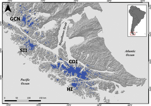
Santa Inés Island is located southwest of the Strait of Magellan, close to its entrance to the Pacific Ocean, and is one of the largest islands of the Magallanes Region in Chile (Figure 1). The central area of the island hosts a significant icefield (Shipton 1963), the Santa Inés Icefield (53° 47ʹS, 72° 35ʹW), one of the main glacier areas of the region, with 168 ± 5 km² in accordance to the Fuego-Patagonian Andes glacier inventory of 2017 (Meier, Hochreuther, and Braun 2018), who also described the other glacier areas in Southern Patagonia: Gran Campo Nevado (189 ± 5 km²), Cordillera Darwin Icefield (2,931 ± 155 km²), and Cloue Icefield on Hoste Island (203 ± 6 km²). Bown et al. (2014) compiled the first detailed glacier inventory south of the Strait of Magellan using satellite images from 2011 and before. This inventory includes 1,681 glaciers, distributed on the Isla Grande de Tierra del Fuego (2,606.2 km²), Hoste Island (409.5 km² including adjacent islands), and Santa Inés Island (273.8 km² including adjacent islands). Masiokas et al. (2009) reported that the Santa Inés Icefield is one of the least studied glacier areas in the region, a shortcoming that we address in this work. Although temperatures in the Southern Andes are relatively temperate, particularly at the elevations of Santa Inés Icefield (maximum 1,500 m a.s.l.), glaciers here persist mainly due to the heavy precipitation caused by the westerlies, although available precipitation estimates vary considerably (Sauter 2020).

Figure 1. Glacier areas in Southern Patagonia: Gran Campo Nevado (GCN), Santa Inés Icefield (SII), Cordillera Darwin Icefield (CDI), and Cloue Icefield on Hoste Island (HI).

Few expeditions and explorations have been carried out at Santa Inés Island, and only a handful have accessed its interior (i.e., Saint-Loup 1952; Bruchhausen 1966; Mortensen 1965; Miller 1967; Peters 1987). This lack of exploratory and field research activity is mainly due to the access difficulties and the harsh climatic conditions characteristic of the area. During the aerial Trimetrogon survey of Chile by the U.S. Photographic Squadron in 1944 and 1945, the dense and persistent cloud cover left Santa Inés as the only area in Chile without complete photographic coverage (Miller 1965; Lliboutry 1999). In 2001, Veijo Pohjola (unpublished, personal communication) performed measurements on Hooke Glacier, and Aravena (2007) studied the frontal moraines of two outlet glaciers: Hooke (which he refers to as Alejandro) and Beatriz. Finally, in January 2019, Isaac Gurdiel and Paulo Rodríguez explored and surveyed parts of the outlet glacier between Hooke/Alejandro and Beatriz, which they refer to as Glaciar Nati (Figure 2).

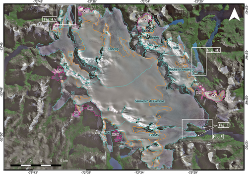
Figure 2. Glacier inventory (2020) displayed over a Sentinel-2 image from 31/03/2017 using a real color composition with the saturation enhanced using the near-infrared band. The turquoise outlines represent the 12 glaciers selected for the analysis of area changes (1945–2020) and thickness changes (2000–2014); the purple outlines correspond to the remaining glaciers of the Santa Inés Icefield; and orange lines are the 2017 ELA of each glacier.

This work builds upon the MSc thesis by Gurdiel (2019) and aims to improve our limited knowledge of one of the least studied icefields in Southern Patagonia. For this purpose, we have compiled a detailed glacier inventory of the Santa Inés Icefield by manual digitization of glacier outlines using high-resolution satellite images and aerial photographs. Although our glacier inventory is not the first on Santa Inés Island and the last published, from 2017, is quite recent (Meier, Hochreuther, and Braun 2018), ours is the first of the icefield only (Santa Inés Icefield), which is very important for comparing with other icefields or continuous ice masses of the region (Figure 1). In addition, we have determined the area changes of several glaciers of the Santa Inés Icefield between 1945 and 2020. The TanDEM-X (2014) data from Braun et al. (2019) have been integrated into this analysis for calculating changes in glacier surface elevation compared to the SRTM (2000) data set. Finally, we have investigated possible climatic drivers of these changes using ERA5 reanalysis data of surface and 850 mb fields (temperature, precipitation), since there are no weather stations on Santa Inés Island and only a few in Southern Patagonia, which are mainly located to the east of the Andes. The great west-east climatic variability in the Southern Andes hampers the use of the existing weather station data to infer the conditions on the Santa Inés Icefield (Carrasco, Casassa, and Rivera 2002; Aravena and Luckman 2009; Aguirre et al. 2018; Weidemann et al. 2018). Our results have been compared with the recently published glacier inventory of the Fuego-Patagonian Andes of Meier, Hochreuther, and Braun (2018), obtained by semi-automated methods, allowing a comparison with our manually-obtained results. The recent variations of Santa Inés Icefield have been compared with other glacier surfaces in Southern Patagonia (Figure 1) to verify if Santa Inés Icefield glaciers are following the continuous glacier retreat and shrinking published by several authors (Lopez et al. 2010; Meier, Hochreuther, and Braun 2018; Braun et al. 2019; Masiokas et al. 2020; Hugonnet et al. 2021).

Data and methods

Cartographic method for glacier inventory

We have updated previous inventories of the Santa Inés Icefield (Bown et al. 2014; Dirección General de Aguas de Chile – DGA 2014; Randolph Glacier Inventory (RGI) Consortium 2017; Meier, Hochreuther, and Braun 2018) based on the analysis of Sentinel-2 optical satellite imagery, which was launched in 2017 and acquires images with 10 m ground resolution (Gascon et al. 2014). While Sentinel-2 has five-day revisit time, cloud cover or high surface snow cover renders most available images unusable for glacier delineation. The best image found to optically delineate glacier outlines was acquired on 31st of March 2017; having been acquired at the end of the austral summer with minimum cloud and snow cover, it allowed us to map the entire icefield. RGI inventory 6.0 data over Santa Inés used Advanced Spaceborne Thermal Emission and Reflection Radiometer (ASTER) images from 2000 and 2003. Bown et al. (2014) inventoried Santa Inés Island and adjacent islands (273.8 km²) using an ASTER image from 2005. Meier, Hochreuther, and Braun (2018) published Santa Inés Island (168 ± 5 km²); however, none of these inventories determined Santa Inés Icefield as a continuous ice mass that constitutes an icefield. For all glaciers in the Santa Inés Icefield we have also updated the lower glacier areas and terminus positions using two Sentinel-2 images from 04/02/2019 and 07/02/2020, acquired in mid-summer but which present more snow cover than the 31/03/2017 image (Table 1).

Table 1. Aerial photographs and satellite images used for the glacier inventory and area changes of Santa Inés Icefield. Imagery sources are United States Aerial Force (USAF); United States Geological Survey (USGS); European Space Agency (ESA).

Aerial photographs
Sensor Date and Photo	Sensor	Source
09/03/1945 (91PC 5 M 4028 461.R.44)	USAF Trimetrogon survey	University of Magallanes
09/03/1945 (91PC 5 M 4028 461.R.45)
09/03/1945 (91PC 5 M 4028 461.R.46)
Satellite images
Date	Sensor	Source
04/05/1978	Landsat-3 MSS	USGS
06/10/1986	Landsat-5 TM	USGS
02/02/1998	Landsat-5 TM	USGS
28/02/1999	Landsat-5 TM	USGS
19/03/2000	Landsat-7 ETM+	USGS
25/03/2002	Landsat-7 ETM+	USGS
03/10/2005	Landsat-5 TM	USGS
23/01/2009	Landsat-7 ETM+	USGS
15/12/2011	Landsat-7 ETM+	USGS
23/01/2015	Landsat-8 OLI	USGS
31/03/2017	Sentinel-2	ESA
04/02/2019	Sentinel-2	ESA
07/02/2020	Sentinel-2	ESA

Image processing was customized to improve visualization and highlight the differences between the terrain types found in western Patagonia. This processing consists of a real color RGB composite (bands 4-3-2), where saturation is adjusted using the saturation values of a near-infrared RGB combination (bands 8-4-3). This process highlights the vegetation and recovers detail in shadow areas. In particular, this processing made glacier boundaries perfectly clear in our images, also allowing the identification of other land types. Therefore, it was not necessary to enhance ice/snow contrast using the normalized difference snow index (NDSI), which is commonly used for outlining glaciers. Nunataks from recently deglaciated areas or not detected in previous inventories have been accounted for to obtain the real ice surface of Santa Inés Icefield. During the manual digitization of each glacier, we assumed a horizontal error of ± 1 pixel (Williams et al. 1997; Meier, Hochreuther, and Braun 2018) corresponding to ± 10 m (spatial resolution of used Sentinel-2 bands). The use of cloud-free images with minimal snow cover allowed us to accurately identify and digitize the glacier boundary. Therefore, we assume the error in the glacier boundary digitization to be equal to the spatial resolution of the satellite imagery used. Thus, the absolute error in the area estimation of a glacier increases with the perimeter of the glacier. Following the buffer method proposed by Granshaw and Fountain (2006), we assume the error is equal to the area of a buffer band around the perimeter of the glacier of width equal to the pixel-by-pixel root-mean-square error (RMSE). Therefore, if the spatial resolution of the imagery is R and P the perimeter of the glacier, we consider the area to be defined by a polygon made of P/R vertices, each with a position error of R. This defines a root-mean-square error of

(1) $RMSE=\frac{\sqrt{R^2\frac{P}{R}}}{\frac{P}{R}}\left[m\right]=\frac{\sqrt{RP}\times R}{P}\left[m\right]$(1)

The total area error is then calculated as the area of a buffer band of width RMSE and length P, which for simplicity and without introducing significant differences, is calculated as the area of a rectangle of sides P and RMSE. In this way, the total area error E is assumed to be equal to

(2) $E=\sqrt{RP}\times R\left[m^2\right]$(2)

To aid in the determination of the divide between the upper areas of the different outlet glaciers of the Santa Inés Icefield, we have used aspect and slope maps generated from a TanDEM-X (2014) digital elevation model, with 30 m spatial resolution.

We have compiled a glacier inventory database for the Santa Inés Icefield with 15 attributes (Table 2), of which 12 (RGIId, Date, CenLon, CenLat, 01Region, Area, GlacType, Exposition, Name, Z_min, Z_max, L_max) correspond to RGI 6.0 attributes (RGI Consortium 2017). We have included the following three additional attributes that we consider relevant: Equilibrium Line Altitude (ELA), mean surface elevation (Z_ave), and Accumulation Area Ratio (AAR). The snow line at the end of the summer for temperate glaciers in the Southern Hemisphere is a proxy to determine the ELA (Rivera et al. 2007; Barcaza et al. 2009). Using this approach, we digitized the ELA on the Sentinel-2 image from 31/03/2017 (Figure 2) using a near-infrared false color composite (bands 8A-4-3), and we calculated the average altitude of the digitized line for each glacier based on the TanDEM-X (2014) digital elevation model. Z_ave corresponds to the mean elevation of each glacier that is not provided explicitly in the RGI (RGI Consortium 2017). From the ELA, we have the ablation (Aa) and accumulation areas (Ac), and we calculated the AAR based on the function AAR = Ac/(Ac+Aa) (Cogley et al. 2010). Although we recognize the limitation of extracting the ELA from a single date, it provides a reasonable way of evaluating the AAR, which has been linked to glacier behavior (De Angelis 2014). The database fields (Table 2) corresponding to the topographic information (Z_min, Z_max, Zmed) have also been calculated from the TanDEM-X (2014) digital elevation model. The band composition and image adjustment have been done using Adobe Photoshop CC 2018 software, due to its image manipulation tools and its capacity to recover appropriate detail in both shaded and bright areas within a 16-bit image. The digitization of the glacier outlines and the database development was done with Quantum GIS (Geographic Information Systems) 3.10.1.

Table 2. Glacier inventory. Randolph Glacier Inventory ID (RGIID); (01Region) first order region number; (GlacType) land-terminating (0), freshwater (1), tidewater (2); (L_max) length of the longest surface flowline of each glacier; (Z) minimum, maximum, and average elevation of each glacier; Accumulation-Area Ratio (AAR).

	Name	RGIID	CenLat	CenLon	O1Region	Date	GlacType	Exposition	Area (km^2)	ELA (m)a	Lmax (m)	Zmin(m)	Zmax(m)	Zave (m)	AAR*
	I	RGI60-17.03489	−53.734038°	−72.674493°	17	07/02/2020	1	N	1.70 ± 0.40	544	3,381	129	847	460	0.37
	II	RGI60-17.03465	−53.740517°	−72.692491°	17	07/02/2020	0	N	0.30 ± 0.19	701	1,390	636	1,025	809	0.84
	III	RGI60-17.03457	−53.765598°	−72.669590°	17	07/02/2020	0	W	13.64 ± 0.71	710	8,787	144	1,243	671	0.35
	IV	RGI60-17.03428	−53.779341°	−72.685694°	17	07/02/2020	0	NW	0.41 ± 0.21	931	1,421	701	1,139	937	0.72
	V	-	−53.785661°	−72.682414°	17	07/02/2020	0	SW	0.99 ± 0.26	890	1,987	558	1,123	877	0.97
	VI	RGI60-17.03412	−53.799193°	−72.663868°	17	07/02/2020	1	SW	6.20 ± 0.40	995	5,088	38	1,284	834	0.80
	VII	-	−53.816669°	−72.656997°	17	07/02/2020	0	S	0.35 ± 0.22	-	1,654	383	1,030	720	0
	VIII	-	−53.812180°	−72.637540°	17	07/02/2020	0	SE	1.66 ± 0.31	-	3,711	154	1,122	908	0
	IX	RGI60-17.03368	−53.833483°	−72.608952°	17	07/02/2020	1	S	2.79 ± 0.38	1,063	3,844	344	1,287	849	0.73
	X	RGI60-17.03362	−53.842179°	−72.573888°	17	07/02/2020	1	SW	2.41 ± 0.35	946	2,994	390	1,271	889	0.21
	XI	RGI60-17.03348	−53.854233°	−72.532419°	17	07/02/2020	0	S	4.98 ± 0.36	752	3,835	315	1,065	686	0.41
	Helado	RGI60-17.03379	−53.833911°	−72.539906°	17	07/02/2020	0	E	10.63 ± 0.49	773	7,035	6	1,272	756	0.53
	Sarmiento de Gamboa	RGI60-17.03438	−53.804113°	−72.548263°	17	07/02/2020	0	SE	46.96 ± 0.75	691	13,542	4	1,293	742	0.60
	XIV	-	−53.793313°	−72.472648°	17	07/02/2020	0	SW	0.38 ± 0.23	779	1,975	615	830	762	0.23
	XV	-	−53.796917°	−72.451491°	17	07/02/2020	0	N	1.57 ± 0.31	873	3,233	521	1,188	847	0.77
	Hooke or Alejandro	RGI60-17.03446	−53.774875°	−72.501246°	17	07/02/2020	1	NE	7.60 ± 0.44	716	5,421	74	1,164	766	0.73
	Nati	RGI60-17.03449	−53.756219°	−72.511011°	17	07/02/2020	0	NE	2.27 ± 0.33	578	3,484	195	1,123	770	0.82
	Beatriz	RGI60-17.03467	−53.747485°	−72.543935°	17	07/02/2020	1	NE	5.51 ± 0.57	723	4,770	55	1,134	716	0.51
	XIX	-	−53.739551°	−72.567660°	17	07/02/2020	0	S	0.17 ± 0.15	-	819	822	972	911	0
	XX	RGI60-17.03472	−53.731745°	−72.559754°	17	07/02/2020	0	N	0.98 ± 0.23	807	1,707	477	1,032	865	0.87
	Snoring	RGI60-17.03474	−53.758820°	−72.605105°	17	07/02/2020	2	N	36.65 ± 0.70	619	12,148	21	1,220	703	0.67
	XXII	RGI60-17.03475	−53.726745°	−72.649777°	17	07/02/2020	0	N	0.87 ± 0.28	772	2,344	484	797	729	0.84
	XXIII	-	−53.740117°	−72.662650°	17	07/02/2020	0	N	0.29 ± 0.17	-	1,085	492	778	723	0
	XXIV	-	−53.836520°	−72.590473°	17	07/02/2020	0	SW	0.48 ± 0.29	-	1,713	585	1,240	948	0
Santa Inés Icefield			−53.783333°	−72.583333°	17	07/02/2020	-		149.31 ± 1.84	782	-	4	1,293	787	0.50

* Glaciers VII, VIII, XIX, XXIII, and XXIV do not have an ELA value because their snow line at the end of the summer (31/03/2017) was above the maximum elevation of the glacier, and therefore, their AAR is equal to 0. The ELA and AAR of the Santa Inés Icefield (782 m and 0.50) correspond to the average for the entire inventory.

Optical satellite images, aerial photographs, and digital elevation models for assessing glacier changes

Based on our glacier inventory, we have determined frontal variations between 1945 and 2020 using multiple optical satellite images and aerial photographs (Table 1). Due to the scarcity of cloud-free summer images, we have used winter satellite images as well, in order to increase the spatial and temporal coverage of the frontal variations record. With the available imagery, we were able to determine the variations of 12 of the 24 glaciers included in our inventory. These 12 glaciers cover an area of 141.34 ± 5.6 km² (94.7 percent of the Santa Inés Icefield 2020 total area of 149.31 ± 5.8 km²), including all 3 types of glacier fronts present in the area (freshwater, tidewater, and land-terminating) and covering all slope aspects (north, south, east, and west). Therefore, we consider that these 12 glaciers are representative of the Santa Inés Icefield evolution during the analyzed period. Due to cloud cover in some photographs and satellite images, not all glaciers have their frontal positions delimited within the study period (Table 3).

Table 3. For the 12 selected glaciers: Surface area (km²), area change (km²; %), and annual change (km² a⁻¹) for the longest period available; thickness changes (ma⁻¹; 2000–2014) obtained from SRTM (2000) and TanDEM-X (2014) digital elevation models.

Glacier	1945	1978	1986	1998	1999	2000	2002	2005	2009
I	-	-	3.69 ± 0.80	3.17 ± 0.77	-	-	3.11 ± 0.53	2.95 ± 0.76	-
III	-	-	-	16.04 ± 1.22	15.60 ± 1.22	-	-	15.46 ± 1.25	-
VI	-	-	-	6.83 ± 0.75	6.83 ± 0.75	6.83 ± 0.47	6.83 ± 0.47	6.83 ± 0.75	6.21 ± 0.46
IX	-	5.19 ± 1.14	-	5.07 ± 0.69	5.03 ± 0.68	-	5.03 ± 0.50	5.03 ± 0.68	-
X	-	2.98 ± 1.20	-	2.87 ± 0.74	2.82 ± 0.73	2.82 ± 0.53	2.82 ± 0.53	2.83 ± 0.73	-
XI	-	6.08 ± 1.15	-	-	5.88 ± 0.70	-	5.99 ± 0.49	5.84 ± 0.68	-
Helado	10.71 ± 0.60	-	-	-	10.68 ± 1.00	-	-	10.68 ± 1.00	-
Sarmiento de Gamboa^+	46.77 ± 0.60	-	-	-	46.73 ± 1.41	-	46.73 ± 1.02	46.72 ± 1.41	-
Hooke or Alejandro	-	-	8.82 ± 0.88	8.60 ± 0.86	-	-	8.40 ± 0.70	8.44 ± 0.84	7.89 ± 0.62
Nati	-	-	2.88 ± 0.63	2.60 ± 0.64	-	-	2.62 ± 0.49	2.76 ± 0.61	-
Beatriz	-	-	6.45 ± 1.02	5.98 ± 0.99	-	5.96 ± 0.82	-	5.89 ± 0.97	-
Snoring	-	-	37.05 ± 1.33	36.67 ± 1.33	-	36.64 ± 0.84	36.45 ± 0.84	36.65 ± 1.33	-
Santa Inés Icefield		-	-	151.12 ± 3.29		-	-	150.08 ± 3.30	-
Glacier	2011	2015	2017	2019	2020	Area change (km^2)	Area change (%)	Annual Change (km^2 a^−1)	Mean elevation change dh/dt ± 0.26 (ma^−1) 2000–2014
I	-	2.58 ± 0.51	2.32 ± 0.42	1.80 ± 0.39	1.70 ± 0.40	−1.99 ± 0.40	−53.9	−0.06 ± 0.01	−2.90
III	-	-	13.97 ± 0.68	13.88 ± 0.67	13.64 ± 0.71	−2.40 ± 0.51	−15.0	−0.11 ± 0.02	−0.75
VI	-	6.27 ± 0.46	6.26 ± 0.38	6.22 ± 0.37	6.20 ± 0.40	−0.63 ± 0.35	−9.2	−0.03 ± 0.02	0.06
IX	4.91 ± 0.49	-	2.85 ± 0.36	2.83 ± 0.36	2.79 ± 0.38	−2.40 ± 0.76	−46.2	−0.06 ± 0.02	−0.59
X	2.82 ± 0.55	2.44 ± 0.48	2.45 ± 0.35	2.44 ± 0.34	2.41 ± 0.35	−0.57 ± 0.85	−19.1	−0.01 ± 0.02	−0.17
XI	5.60 ± 0.48	5.34 ± 0.49	5.10 ± 0.35	5.08 ± 0.34	4.98 ± 0.36	−1.10 ± 0.69	−18.1	−0.03 ± 0.02	−0.92
Helado	10.67 ± 0.70	-	10.61 ± 0.48	10.62 ± 0.48	10.63 ± 0.49	−0.08 ± 0.11	−0.8	−0.00 ± 0.00	−0.60
Sarmiento de Gamboa^+	46.77 ± 0.60	-	46.97 ± 0.70	46.92 ± 0.72	46.96 ± 0.75	0.19 ± 0.15	0.3	0.00 ± 0.00	−0.09
Hooke or Alejandro	-	-	7.68 ± 0.44	7.60 ± 0.44	7.60 ± 0.44	−1.22 ± 0.44	−13.8	−0.04 ± 0.01	−0.54
Nati	-	-	2.30 ± 0.30	2.30 ± 0.30	2.27 ± 0.33	−0.61 ± 0.30	−21.2	−0.02 ± 0.01	−0.38
Beatriz	-	5.81 ± 0.68	5.60 ± 0.52	5.56 ± 0.52	5.51 ± 0.57	−0.94 ± 0.45	−14.6	−0.03 ± 0.01	−0.44
Snoring	-	-	36.95 ± 0.68	36.63 ± 0.68	35.65 ± 0.70	−1.40 ± 0.63	−3.8	−0.04 ± 0.01	0.16
Santa Inés Icefield		-	142.76 ± 1.70	141.88 ± 1.70	141.34 ± 1.77	−9.78 ± 1.53	−6.5	−0.45 ± 0.07	−0.60

⁺Glaciers XI, Helado, and Sarmiento de Gamboa do not have available surface area in 1998, so we have taken their positions in 1999 for estimating the Santa Inés Icefield surface area in 1998.

The aerial photographs, taken during the austral summer, are three oblique images mostly cloud covered but clear at the front of two of the main and biggest glaciers of Santa Inés Icefield (Helado and Sarmiento de Gamboa, Table 2), that end at Seno Helado (Figure 2; Table 3). Because of the cloud cover, we could only digitize manually the frontal and the lower parts of the glacier tongue, by visual comparison of old and recent imagery using as reference all the unchanged features in the surrounding landscape. For estimating the error we have digitized multiple (3) times each glacier following the method of Tielidze and Wheate (2018), obtaining an uncertainty of 5.5 percent corresponding to an error of ± 0.60 km². In the case of satellite images, we have estimated the error using the same method described in Section 2.1, following the method proposed by Granshaw and Fountain (2006).

To measure the Santa Inés Icefield surface elevation changes, we have compared the altitude differences between SRTM (year 2000) and TanDEM-X (year 2014) digital elevation models, both at 30 m spatial resolution. We applied the methodology described by Malz et al. (2018) and Braun et al. (2019), which first corrects both Digital Elevation Measurements (DEMs) vertically and horizontally by applying systematic offsets in stable off-glacier areas following the method developed by Nuth and Kääb (2011). Subsequently, differences on glaciated areas are attributed to surface elevation change (Δh). Assuming that ice-free areas have not changed their altitude between 2000 and 2014, we have calculated the average standard deviation of the differences for the ice-free zones, obtaining a value of σ = 0.13 m/a, which we assume to be representative of the error in Δh over glaciers. The thickness changes have been analyzed on the same 12 glaciers for which we have computed frontal variations. In our analysis, we consider glacier thickening or thinning are statistically significant if Δh is equal or greater than 2σ; therefore, glaciers that show rates of elevation change between +0.26 and −0.26 m/a (2σ) have not been assigned a thinning/thickening trend. This estimated statistical significance of glacier thickening or thinning is quite conservative according to Rolstad, Haug, and Denby (2009), and this error estimate is likely to be an overestimation. While we rather overestimate than underestimate errors, we might be overlooking the significance of some of the smaller thinning trends.

Climatic data

To explore the relationships between the observed changes in the Santa Ines Icefield during the study period and climatic variables, we have used ERA5 reanalysis data (Copernicus Climate Change Service 2019). This dataset spans from 1978 to 2018, covering the whole Earth surface with a grid cell size of approximately 30 × 30 km and with 137 atmospheric levels from the surface to 80 km of altitude. The four ERA5 grid cells closest to Santa Inés Icefield are as follows: NW (−53.75°S, −72.75°W), NE (−53.75°S, −72.50°W), SW (−54.00°S, −72.75°W), and SE (−54.00°S, −72.50°W). At these locations, we have analyzed the following five climatic variables: Surface temperature (monthly average in °C), surface positive degree days (PDD) (accumulated annually in °C day), temperature at 850 mb (monthly average in °C), and precipitation (accumulated annually in mm). The 850 mb isobar corresponds to approximately 1,400 m of elevation, which is the closest atmospheric level of ERA5 to the maximum elevation of the Santa Inés Icefield (1399 m; Miller 1969). The PDD corresponds to the number of positive degrees per day and constitutes a standard proxy to estimate melting rates (Braithwaite and Olesen 1989; Wake and Marshall 2015).

To analyze the robustness of the trends shown by linear regression of the observations of climatic variables, we have applied a significance test with t-statistic using a p-value of 5 percent. Additionally, for validation purposes, we have compared the ERA5 reanalysis temperature data at 850 mb in Punta Arenas with radiosonde data in the period 2000–2016.

Response time to climate forcing

To properly understand the relationship between climate and glacier variations, we need to consider the response time of the different glaciers to climate forcing. A first approximation to the response time T according to Jóhannesson et al. (1989) is given by

(3) $T=\frac{H}{-Ab}{}_{[years]}$(3)

where H is the average thickness of the glacier and Ab the rate of the ablation along its terminus. Although we do not know the value of these parameters for the Santa Inés Icefield glaciers, we calculated a rough order-of-magnitude estimation using the ablation rate at the terminus of the nearby Glaciar Schiaparelli in the Mount Sarmiento Massif (Cordillera Darwin Icefield, Figure 1) and an area-volume scaling relationship. Weidemann et al. (2020) measured the ablation rate near the terminus of Glaciar Schiaparelli using ablation stakes and resulting in approximately −6 m w.e. per year. We have estimated the average thickness H, simply as the ratio between estimated volume V and the surface area A:

(4) $H={\frac{V}{A}}_{[m]}$(4)

The volume of a glacier can be estimated by using scaling relationships (Radic and Hock 2010; Bahr et al. 2015) of the form

(5) $V=c\times A^y[k{m}^3]$(5)

where c is a glacier-dependent scaling parameter and y a scaling exponent that can be derived analytically. Bahr et al. (2015) recommends fixing the scaling exponent to its theoretical value of y = 1.375, and adjusting the value of c to fit specific datasets. Given that we do not have data to derive an experimental value of the scaling parameter c tailored to glaciers similar to the Santa Inés Icefield, and that this value has relatively small variations between glaciers, spanning only one order of magnitude (Bahr et al. 2015). We will adopt the value used globally by Radic and Hock (2010) corresponding to c = 0.2055 m^3−2y.

Results

Glacier inventory

The glacier inventory is presented in Table 2 and Figure 2, with the terminus position of all glaciers being updated to the most recent image (February 2020). In the absence of official names for these glaciers, we have used names coined by previous researchers or by us, none of which are officially recognized yet by the Chilean mapping agency (Instituto Geográfico Militar). Glaciar Helado was named as such because it terminates in Seno Helado. Glaciar Snoring was named by Miller (1967), Glaciar Beatriz by Aravena (2007), and Glaciar Hooke or Alejandro by Pohjola (2001, unpublished, personal communication) and Aravena (2007), respectively. Glaciar Nati was named by Isaac Gurdiel and Paulo Rodríguez during their January 2019 fieldwork campaign (Gurdiel 2019); Glaciar Sarmiento de Gamboa was named after the Spanish navigator who named Santa Inés Island and is used by visitors to the area. We have used roman numerals for unnamed glaciers. The glacier inventory has 24 glaciers and 15 associated fields in the database (Table 2), with a total area of 149.31 ± 1.84 km² (07/02/2020).

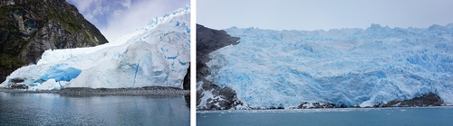
The inventory we present here, as well as the previous ones, are based on remote sensing techniques, which constitute a valuable tool to study remote areas. However, these techniques require field observations for validation and to observe details not visible in the imagery due to resolution or perspective. During our field campaign between December 2018 and January 2019 to Santa Inés Island, we observed that Helado and Sarmiento de Gamboa glaciers are land-terminating, with their terminus fully underlaid by bedrock in the case of Sarmiento de Gamboa, and exhibiting a small 1 m high frontal moraine in the case of Helado (Figure 3). This detail escaped from satellite image observations due to the short distance (less than 10 m) that separated the respective glacier fronts from the fjord waters. While they may have recently ceased to calve, the lack of available imagery with resolution high enough to appreciate such details, and the fact that their frontal positions do not show significant changes since 1945, suggest that they probably became land-terminated glaciers a long time ago. The inventories of Bown et al. (2014), DGA (2014), RGI Consortium (2017), and Meier, Hochreuther, and Braun (2018) classify both of these glaciers as tidewater.

Figure 3. Fronts of Helado (left) and Sarmiento de Gamboa (right) glaciers in December 2018. Photographs by Paulo Rodríguez.

Area and surface elevation changes

Area changes for different periods between 1945 and 2020 and surface elevation changes (2000–2014) have been determined for 12 of the 24 glaciers of the Santa Inés Icefield (Figure 2, Table 3). The time series of area changes for the 12 selected glaciers cover the time period between 1945 and 2020, although with multiple data gaps prior to 2005, the first year in which Santa Inés Icefield is completely covered in the same date due to lack of cloud-free imagery (Table 3). Surface area estimations are available for all 12 glaciers simultaneously for years 2005, 2017, 2019, and 2020. For year 1998, Santa Inés Icefield area has been estimated with the surface area available for 9 glaciers in 1998, and adding the surface area available next year (1999) of the other three glaciers (XI, Helado, and Sarmiento de Gamboa), being 151.12 ± 3.29 km² (Table 3), assuming that these three glaciers have not changed a lot in only one year. Due to the lack of photographs available and the cloud cover of the three aerial photographs that we have, we could only estimate for 1945 the frontal position of two of the twelve glaciers analyzed (Helado and Sarmiento de Gamboa; Table 3).

Table 4 shows the total surface area of the studied glaciers in all available dates, as well as the annual changes for the longest period available at each glacier. The total surface area estimates of the Santa Inés Icefield is presented for years on which we have surface data for all its twelve main constituting glaciers. Note that the earlier estimate combines images from 1998 and 1999. Due to the irregular data availability, the time intervals used for the total surface area change on each glacier is different and not suitable for direct comparison. Instead, the rate of change (km² a⁻¹) offers a clearer picture of the spatial patterns of glacial changes. However, these values are also affected by the different time intervals covered, in particular for the glaciers with surface data available on earlier imagery dated between 1945 and 1986. In the earliest period with surface data for the whole Santa Inés Icefield (1998–2005) the surface area was changing at an annual rate of −0.15 ± 0.01 km² a⁻¹, which increased significantly in the most recent period (2005–2020) to −0.58 ± 0.10 km² a⁻¹ for 2005–2020. This increase in the rate of area change of Santa Inés Icefield strongly suggests a significant acceleration in the glacier retreat, especially during the last 15 years (2005–2020), with a rate of change almost four times larger than in the previous 7 years. Between 1998 and 2020, the Santa Inés Icefield has −9.78 ± 1.52 km², at an annual rate of −0.45 ± 0.22 km² a⁻¹. Unfortunately, the two glaciers with area values for 1945 (Table 3, Figure 5), which account for 38.6% of the Santa Inés Icefield surface in 2020, are not representative of the whole icefield; instead, they are the ones displaying the smallest changes. However, we estimate the lower limit to the Santa Inés Icefield surface area loss to be approximately −13 km² between 1945 and 2020 (75 years). Given that we do not have data for 1945 in ten out of the twelve glaciers analyzed, we have estimated this lower limit of area change by adding the area change of each glacier between the first year with data available and 2020 (Table 3). In other words, we have assumed that glaciers with no data had a constant surface area between 1945 and our first area estimation of each. Therefore, in the context of a long-term glacier reduction, this area change estimation is most likely a lower limit, and a longer area might have been lost. We have refrained from adding an error figure to this estimation. While the error in our determination of the measured area is ±1.5 km², we have no means to constrain the error associated with the period without data. Consistent with this glacier area reduction of the Santa Inés Icefield, our results show an average surface lowering of −0.60 ± 0.26 m a⁻¹ between 2000 and 2014 (Table 3).

Table 4. Surface area variation and annual change for the periods with the whole Santa Inés Icefield surface area estimated.

Period	Years	Area change (km^2)	Area change (%)	Annual change (km^2 a^−1)	Annual change (% a^−1)
1998–2005	7	−1.04 ± 0.11	−0.7	−0.15 ± 0.01	−0.1
1998–2020	22	−9.78 ± 1.52	−6.5	−0.45 ± 0.22	−0.3
2005–2020	15	−8.74 ± 1.53	−5.8	−0.58 ± 0.10	−0.4

An individual analysis of the studied glaciers shows that three glaciers remained stable (area change <4 percent), and these are Snoring (−3.8 percent, −1.40 ± 0.63 km², 1986–2020), Helado (−0.8 percent, −0.08 ± 0.11 km², 1945–2020), and Sarmiento de Gamboa (an increase of +0.4 percent, +0.19 ± 0.15 km², 1945–2020) (Table 3, Figure 5). These glaciers are some of the largest glaciers of Santa Inés Icefield (first, second, and fourth; Table 2) with an area of 93.24 km², which means the 66 percent of Santa Inés Icefield area in 2020. The other nine glaciers display significant area losses ranging from 9.2 percent to 53.9 percent (Table 3). Most of these nine glaciers have lost between 9 percent to 20 percent of their surface area, and only three glaciers have lost more than 20 percent: Glaciar Nati lost 21.2 percent (−0.61 ± 0.30 km²), Glaciar IX lost 46.2 percent (−2.40 ± 0.76 km²), and Glaciar I shows the largest retreat with the loss of more than half of its initial surface area (53.9 percent; −1.99 ± 0.40 km²; Table 3, Figure 4a).

Figure 4. Area changes (1986–2020) and thickness changes (2000–2014) of Glaciar I (Figure 4a) and Glaciar Hooke or Alejandro (Figure 4b). Thickness changes reflect an average for the whole glacier, including ablation and accumulation areas. Background image Sentinel-2 of 31/03/2017. Note that Glaciar Hooke or Alejandro (Figure 4b) shows an increase in the area in the upper zone between 1998 and 2005. However, this change most likely corresponds to the presence of seasonal snow, as the only image available for 2005 was from the beginning of austral spring (03/10/2005) when seasonal snow was still present at high elevations.

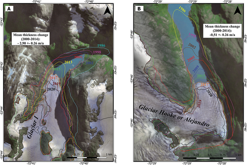
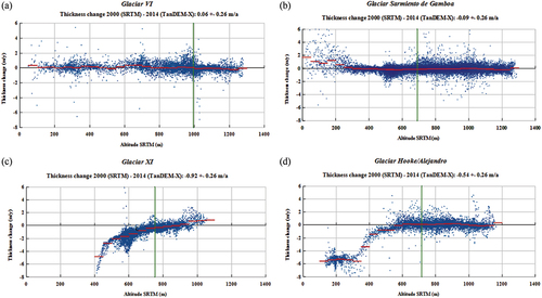
Scatter plots of thickness changes as a function of surface elevation (SRTM) are shown in Figure 6 for four of the twelve glaciers, of which two are stable in terms of surface area change and two have shown an important surface area retreat (Table 3). The thickness changes of VI, X, Sarmiento de Gamboa, and Snoring glaciers do not show significant thickening or thinning (Table 3). This result is consistent with their recent frontal variations in the same period (2000–2014), showing stable surface areas (VI, Sarmiento de Gamboa; Figure 6a,b) and frontal positions (Figure 5; Table 3). I, III, IX, XI, Helado, Hooke/Alejandro, Nati, and Beatriz glaciers show significant loss rates (Table 3), which coincide with their area changes in the same period (2000–2014) as Figure 6c,d shows for XI and Hooke/Alejandro glaciers, characterized by a marked terminus retreat (Table 3, Figure 4b). The zone where the thinning is more pronounced in XI and Hooke/Alejandro glaciers (Figure 6c,d) is below 600 meters of altitude, but in the case of XI glacier it started at 400 meters, while in Hooke/Alejandro glacier it is from 150 meters, which coincides with the longer retreat in the tongue of the Hooke/Alejandro glacier (Figure 4b).

Figure 5. Area changes (1945–2020) and thickness changes (2000–2014) of Helado and Sarmiento de Gamboa glaciers. Thickness changes reflect an average for the whole glacier, including ablation and accumulation areas.

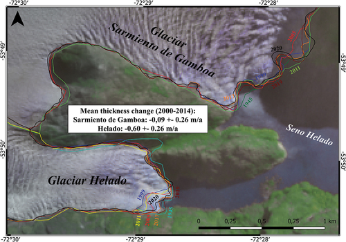
Figure 6. Thickness changes between the years 2000 (SRTM) and 2014 (TanDEM-X). The green line represents the 2017 ELA, and the red lines represent the median values in 50 meters bins to visualize the trends without the influence of outliers.

ERA5 reanalysis and ground station climatic data in 1978–2018

The annual average surface temperature analysis shows differences between the 2 grid cells located west of the Santa Inés Icefield (NW and SW) and those located east (NE and SE). The west side shows a very small warming trend of +0.016°C/y (NW) and +0.017°C/y (SW), while the east shows no trend at all in the period 1978–2018. A similar behavior applies to the accumulated annual PDD (°C day/y), showing different trends between grid cells located to the west, with an increase of +4.54°C day/y (NW) and +4.07°C day/y (SW), while those located on the east show no trend in the 40-year period. The mean PDD over the period 1978–2018 are 1718.6°C day (NW), 1596.4°C day (SW), 1963.0°C day (NE), and 1822.4°C day (SE). For the average annual temperature at 850 mb, there is no trend for any of the four grid cells surrounding the Santa Inés Icefield. This is consistent with the results of Aguirre et al. (2018) that found no trend in temperature in the period 1976–2016 for the 850 mb isobar at Punta Arenas airport. The trend differences for the annual average surface and 850 mb temperature between grid cells located east and west of the Santa Inés Icefield are non-significant (applying a test using a p-value of 5 percent) and are not consistent with the glacier evolution at Santa Inés Icefield during the study period. However, the small, although non-significant values of the accumulated annual surface PDD on the west leave open the possibility that glacier wasting may be forced by atmospheric warming.

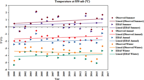
The analysis of annual accumulated surface precipitation in the period 1978–2018 shows different trends between the northern and the southern grid cells. Northern grid cells show an increased rainfall trend of +4.97 mm/y (NW) and +4.93 mm/y (NE), while southern grid cells show a trend of −2.7 mm/y (SW) and −2.6 mm/y (SE), but all four are non-significant trends (applying a p-value of 5 percent). Considering that the total annual rainfall is approximately 3,500 mm, the precipitation change during the study period is not a significant driver for the observed surface and thickness changes. The comparison between ERA5 reanalysis data of annual temperature at 850 mb in the period 2000–2016, with meteorological data observed with radiosonde at 850 mb in Punta Arenas (Figure 7), shows a similar trend of increasing temperature of +0.02°C/y (radiosonde) and +0.02°C/y (ERA5), but both are non-significant (applying a p-value of 5 percent). ERA5 data shows a mean annual temperature 0.48°C, lower than those observed with the radiosonde. Arguably, annual trends might conceal seasonal trends driving glacier change. However, in the Santa Inés Icefield, the seasonal trends present a similar outlook (Figure 7): the summer trend shows an increasing temperature of +0.04°C/y (radiosonde) and +0.02°C/y (ERA5), and while in winter the trend shows a cooling of −0.02°C/y (radiosonde) and a warming trend of +0.02°C/y(ERA5), neither is significant (applying a p-value of 5 percent). This bias is probably due to limitations associated with the lack of upper atmosphere data measurements in the area, with Punta Arenas being the only station in southwestern Patagonia. A recent analysis of surface climate data from ground stations in Patagonia shows significant warming, especially during winter, of up to 0.4°C/decade in the period 1990–2017 (Vilches 2020). This finding confirms the warming reported earlier (Rosenblüth, Fuenzalida, and Aceituno 1997; Carrasco, Casassa, and Rivera 2002; Rasmussen, Conway, and Raymond 2007), being the probable forcing of glacier retreat and thinning in general in glacier surfaces of Southern Patagonia

Figure 7. Average temperature at 850 mb for radiosonde observed data (garnet: summer; red: annual; orange: winter) and for ERA5 reanalysis data (purple: summer; blue: annual; turquoise: winter) at Punta Arenas between 2000 and 2016.

Glacier response time to climate forcing

We estimated the response time to climate forcing of the twelve glaciers selected in the Santa Inés Icefield for the study of the area and surface elevation changes (Table 3). Table 5 shows the surface area, volume, average thickness, and response time of these glaciers. We acknowledge the large uncertainties of this approach, which have been highlighted by many authors (Raper and Braithwaite 2009; Bahr et al. 2015); therefore, the values in Table 5 should be taken only as order-of-magnitude estimates.

Table 5. Surface area, volume, average thickness, and response time of the twelve glaciers analyzed.

Glacier	Surface Area (km^2)	Area change 1998–2020 (m^2 a^−1)	Zmin (m)	Volume V (km^3)	Average thickness H (m)	Response time T (years)
I	1.70	−0.07	129	75.80	44.59	7
III	13.64	−0.11	144	1,327.95	97.36	16
VI	6.20	−0.03	38	449.11	72.44	12
IX	2.79	−0.10	344	149.80	53.69	9
X	2.41	−0.02	390	122.49	50.82	8
XI	4.98	−0.04	315	332.28	66.72	11
Helado	10.63	0.00	6	942.53	88.67	15
Sarmiento de Gamboa	46.96	+0.01	4	7,268.39	154.78	26
Hooke ó Alejandro	7.60	−0.06	74	594.20	78.18	13
Nati	2.27	−0.03	195	112.81	49.70	8
Beatriz	5.51	−0.04	55	381.85	69.30	12
Snoring	35.65	−0.06	21	4,976.15	139.58	23

Discussion

Comparison with previous inventories

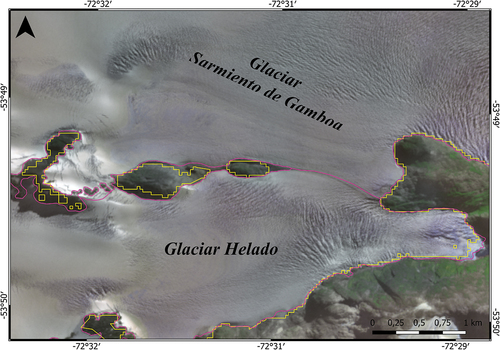
Santa Inés Island glaciers have been inventoried in four studies during the last years (Bown et al. 2014; DGA 2014; RGI Consortium 2017; Meier, Hochreuther, and Braun 2018), but none of these inventories have singularized the Santa Inés Icefield as a continuous ice mass and considered the extension and processes of the icefield as we have done in this study. Meier, Hochreuther, and Braun (2018) used the same Sentinel-2 image as us (31/03/2017), along with a more recent Landsat-8 image (05/11/2017). However, we consider that the latter image is not suited for inventorying purposes, since it shows significant snow cover, probably as a result of early autumn snowfall. We use a more recent image (07/02/2020) to update the areas and terminus positions to February 2020, which shows minimal snow cover. We have compiled the most up to date glacier inventory of the Santa Inés Icefield, and the first considering it as a continuous icefield composed by 24 glaciers (149.31 ± 1,84 km²). We have compared our manual-derived inventory with the semi-automatic version of Meier, Hochreuther, and Braun (2018). Figure 8 shows how the glacier outlines of our inventory present a better fit to the real extent of the glacier surface. This increased accuracy is a direct advantage of the manual method, with the downside of requiring more time. In contrast, the semi-automatic method of Meier, Hochreuther, and Braun (2018) is ideal to perform rapid and effective inventories of larger glacier surfaces, with a lower level of detail. We compared both inventories based on the same image from 2017. Meier, Hochreuther, and Braun (2018) determines an area of 156.51 ± 5 km² and our result shows 151.15 ± 1.70 km², which corresponds to a difference of 3 percent (5.36 ± 3.30 km²) which is compatible with the estimated errors. For large glacier surfaces the semi-automatic method (Meier, Hochreuther, and Braun 2018) is arguably better; however, for increased accuracy on smaller areas our manual method might be a better choice despite being more labor intensive. The difference remains small when comparing individual glaciers; in the case of Glaciar I, we measure 2.32 ± 0.42 km² (Table 3) versus 2.62 km². measured by Meier, Hochreuther, and Braun (2018). The large differences between automated and manually delineated outlines in Figure 8 corresponds to areas in the shadows. This suggests that the advantage of manual delineation is related to the commonalty of conditions challenging for automatic algorithms, such as shaded areas or pack ice, sea ice, or ice melanges in contact with glacier fronts.

Figure 8. Glacier inventory comparison displayed on the Sentinel-2 image of 31/03/2017 using a real color composition with enhanced saturation using the near-infrared band. The staggered yellow line indicates the inventory of Meier, Hochreuther, and Braun (2018), while the pink line shows our glacier inventory.

Glacier change and potential climate forcing

Helado, Sarmiento de Gamboa, and Snoring glaciers are the most stable of the Santa Inés Icefield in terms of frontal position. This could be related with topographic controls, because the Helado and Sarmiento de Gamboa glaciers might benefit from the pinning point provided by the nunatak that separates them, and also from the narrow glacier tongues which favor sidewall drag. In the case of Glaciar Snoring, it is attached to the nunatak that divides its front in two, where it may also be pinned to an underwater anchor point (Koppes, Hallet, and Anderson 2009). However, it is necessary to obtain bathymetry data of Seno Ballena to properly determine the submarine geometry of the area and possible submarine pinning points. For Helado and Sarmiento de Gamboa glaciers, we were able to establish that they had become land-terminating, and the same could be true for Glaciar Snoring, at least on part of its front, which had become increasingly confined in a narrowing fjord. All these factors suggest that small changes observed in these three glaciers could be the result of the stabilizing factor experiencing a reduction or elimination of mass loss due to calving and submarine melting. Further in-depth field studies of the morphology of these glaciers and the bathymetry of their fjords are needed to study the relationship between the morphology of the most stable glaciers and the ground or wall topography. However, the changes in calving previously described suggest that their stability could be mainly associated to internal dynamic processes, in contrast to climatic forcings. These three stable glaciers account for approximately 40 percent of the Santa Inés Icefield surface area.

Despite the relative stability of the three out of the four largest glaciers in the Santa Inés Icefield, we found a generalized surface retreat, with an overall area loss of about 13.19 ± 1.53 km² between 1945 and 2020. This is an approximate figure and most likely an underestimation of the area reduction in this period, as we have assumed negligible change in the period between 1945 and our earlier area estimation for each glacier. We applied this assumption in the ten (out of twelve) glaciers that lack coverage in the 1945 imagery. Additionally, this total area loss estimation only considers 12 of the 24 Santa Inés Icefield glaciers, although these glaciers cover 94.7 percent of the 2020 glaciated area of the icefield. Among the twelve glaciers for which we have analyzed area changes, eight have lost more than 10 percent of their initial surface, with a maximum loss of 53.9 percent for Glaciar I. This glacier has shown a continuous retreat and has split into two different tongues (I, and a new one we refer to as XXIII) between 2017 and 2019.

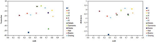
In spite of the general retreat of the Santa Inés Icefield glaciers, the rate of change of its individual glaciers varies significantly, and we were not able to associate this difference to any of their basic characteristics such as the type of glacier front (tidewater, freshwater, land-terminating), minimum elevation (Z_min) or their aspect. We have calculated the AAR for these 12 glaciers and compared it with their area and mean elevation changes (Figure 9), but no clear relationship between these variables was found. Similarly, non-significant correlation was found between area change and terminus slope. In fact, terminus slope values similar to those of the most stable glaciers were found in several of the ones displaying the faster retreats. Moreover, among the glaciers with the largest area loss, we found both steep and shallow terminus slope.

Figure 9. Accumulation Area Ratio (AAR) vs area loss (%) and mean elevation change (ma⁻¹) for the 12 glaciers.

To analyze the total surface area variations of the Santa Inés Icefield, we have selected two periods in which there is available data for all glaciers: 1998–2005 and 2005–2020. Note that for the 1998 area estimation we have used both imagery from 1998 and 1999, surveying nine and three glaciers respectively (Table 3), which might result in an uncertainty larger than represented by our errors. However, this factor is unlikely to significantly modify the calculated area change rates, which are averages over 7 and 15 years, respectively. The annual area changes in the two periods vary from −0.15 ± 0.01 km² a⁻¹ in 1998–2005 to −0.45 ± 0.22 km² a⁻¹ in 2005–2020, in terms of annual percetange change the figures are −0.1% and −0.4 percent, respectively (Table 4). These results are consistent to those of Meier, Hochreuther, and Braun (2018), who published an annual rate from −0.31 percent a⁻¹ (1986–2005) to −0.4 percent a⁻¹ (2005–2016) in the glaciers of Gran Campo Nevado and Santa Inés Island (Figure 1). These results are also in accordance with the accelerated global glacier mass loss in the early twenty first century for the Southern Andes (extended data Table 1 in Hugonnet et al. 2021).

The comparison of the glacier evolution with the available climatic variables at Santa Inés Icefield yields no clear relationship, except for the small increase in the accumulated annual PDD on the western side. The large climatic variability of Southern Patagonia from the Pacific coast to the eastern slope of the Southern Andes (Carrasco, Casassa, and Rivera 2002; Aravena and Luckman 2009; Aguirre et al. 2018; Weidemann et al. 2018), together with the great distance between the Santa Inés Icefield and the nearest weather stations with continuous climatic records, renders reanalysis data as the only suitable source of meteorological information over the Santa Inés Icefield. However, except for the small PDD signal on the west of Santa Inés Icefield and the small warming at 850 mb at Punta Arenas, it has not been possible to find any significant trend using ERA5 reanalysis that could explain the observed area and thickness changes in the Santa Inés Icefield.

The warming recorded in Southern Patagonia during the twentieth century (Rosenblüth, Fuenzalida, and Aceituno 1997; Carrasco, Casassa, and Rivera 2002; Rasmussen, Conway, and Raymond 2007), and more recently (1990–2017) by Vilches (2020), is therefore not clearly reproduced by the ERA5 reanalysis data (1978–2018) of average surface temperature and accumulated annual PDD. The same happens for the temperature at the 850 mb level, where the four grid cells around the Santa Inés Icefield show no significant trends. This is consistent with the absence of significant trends found between 1976 and 2016 at the 850 mb level radiosonde data of Punta Arenas airport (Aguirre et al. 2018).

Regarding precipitation trends, reanalysis data is again our only available data for the Santa Inés Icefield, especially given the great spatial variability of precipitation across Southern Patagonia, the absence of significant trends between stations, and the overall lack of meteorological stations in the region (Carrasco, Casassa, and Rivera 2002; Aravena and Luckman 2009; Aguirre et al. 2018; Weidemann et al. 2018). The most complete precipitation record in the area corresponds to Punta Arenas, showing a notable decrease in accumulated annual precipitation, particularly during the period 1990–2014 (González-Reyes et al. 2017). However, it is not possible to extrapolate these results to the Santa Inés Icefield due to the large west-east precipitation gradient existing in the area (Carrasco, Casassa, and Rivera 2002; Aravena and Luckman 2009; Aguirre et al. 2018; Weidemann et al. 2018). On the other hand, ERA5 reanalysis precipitation data over the Santa Inés Icefield shows no significant trend, suggesting that precipitation is not the driver of the observed changes in the Santa Inés Icefield during the studied period. In the most recent decades, Hugonnet et al. (2021) reports a small increase in precipitation between periods 2000–2009 and 2010–2019; however, we hesitate to take this as supporting evidence because they do not specify if this increase is statistically significant or not.

In the absence of a clear climate forcing in the period 1978–2018 capable of explaining the changes observed in the Santa Inés Icefield as a whole, and considering the wide range of responses observed within its constituting glaciers, we explored other factors in addition to climate forcing. In particular, the magnitude and differences in the response time of these glaciers to such climatic variations. The estimated volume, average thickness and response time of each analyzed glacier are shown in Table 5. Despite the large uncertainties associated (Raper and Braithwaite 2009; Bahr et al. 2015), these estimates are informative about the order of magnitude and the expected differences between glaciers. The comparison between glaciers is especially straightforward for those with their terminus at similar altitudes, and in particular with terminus elevations close to sea level, as is the case of Glaciar Schiaparelli (Cordillera Darwin Icefield, Figure 1), the source of our frontal ablation rate (Weidemann et al. 2020). Therefore, for glaciers with their terminus at higher elevations, we might be underestimating response times, as these glaciers are expected to have smaller ablation rates. Nonetheless, the comparison of response times between glaciers with their terminus at similar altitudes will still be meaningful. Minimum elevations at the Santa Inés Icefield roughly range from 0 to 800 meters (Table 2), and between 0 to 400 meters for the twelve glaciers we have studied in detail (Table 5).

The estimated response time of the twelve analyzed glaciers to climate forcing vary from 7 to 26 years (Table 5), these are relatively short periods compared to the 40 year span of our climatic time series. Therefore, we cannot attribute the observed area thickness changes to climatic trends acting before the start of our analysis in 1978. If such trends existed, the glaciers in the Santa Inés Icefield should have already reached equilibrium. In the light of this conclusion, the changes observed in the Santa Inés Icefield and the different behaviors of its glaciers are most likely related to the combination of internal dynamic processes and climatic trends below our detection threshold. Note that the lack of statistical significance of the observed warming trend does not allow us to discard the existence of such trend; it only prevents us from verifying its existence.

If such climate forcing exists, the aforementioned warming observed in Southern Patagonia (Rosenblüth, Fuenzalida, and Aceituno 1997; Carrasco, Casassa, and Rivera 2002; Rasmussen, Conway, and Raymond 2007; Vilches 2020) stands as the most likely climatic driver behind the observed area reduction and thinning at the Santa Inés Icefield.

Conclusions

Despite the amount of satellite images currently available, the almost constant cloud cover of this region remains a significant obstacle to find useful images to delineate glacier margins. Nonetheless, we have completed the most detailed glacier inventory of the Santa Inés Icefield (Table 2, Figure 8) compiled to date. The findings of our limited field work in the area regarding glacier terminus types (Figure 3), highlights the lack and importance of field data in isolated places, like the remote Santa Inés Icefield in southwestern Patagonia. With a glacier area of 149.31 ± 1.84 km² (07/02/2020), the Santa Inés Icefield presents a generalized retreat trend, although some glaciers show relatively stable terminus positions. The lack of cloud-free imagery or aerial photographs does not allow the frontal positions of many of the glaciers to be obtained during the whole period 1945–2020 especially before the late 1990s. Combining 1998 and 1999 data, we made the earliest estimation of the Santa Inés Icefield area, corresponding to 151.12 ± 3.29 km². After 2000, the availability of cloud-free imagery increased, and we were able to determine the area of the Santa Inés Icefield for the years 2005, 2017, 2019, and 2020. There is room for improvement of the temporal resolution of the area changes by using other satellite images or aerial photographs, such as Satellite Pour l'Observation de la Terre (SPOT) satellite images (1986 onwards) or the Chile60 aerial survey by the Chilean government that imaged the area in 1984. However, we did not have access to these.

The Santa Inés Icefield surface area reduced between 1945 and 2020 by approximately 13 km²; however, this estimate is more likely an underestimation, as we do not have data going back to 1945 for all glaciers, and this figure does not include area losses in periods with no data. Starting from our earlier area estimation of the whole icefield for the years 1998–1999, the total area loss by 2020 was −9.78 ± 1.53 km². In terms of ice thickness change, we found an average thinning of 0.60 ± 0.26 ma⁻¹ (2σ) between 2000 and 2014. It is difficult to compare these results with previous studies on Santa Inés Island because none of the other studies have treated it as an independent continuous glaciaer unit, and it was instead aggregated to other glaciers in Santa Inés and adjacent islands. However, we observe an acceleration of the area loss in the last 15 years in accordance to the results by Meier, Hochreuther, and Braun (2018).

Using the ERA5 reanalysis data, we found no statistically significant warming or precipitation change, that could explain the thinning and area reduction observed on the Santa Inés Icefield. Furthermore, response time estimates suggest that Santa Inés Icefield glaciers are not responding to climatic forcing happening before the period covered by ERA5 reanalysis data. In other locations of western Patagonia, a significant warming signal has been detected by other authors using, especially during winter (Rosenblüth, Fuenzalida, and Aceituno 1997; Carrasco, Casassa, and Rivera 2002; Rasmussen, Conway, and Raymond 2007; Vilches 2020). Therefore, we propose that a slow surface warming trend of magnitude below the detection threshold of ERA5 reanalysis data is the most likely cause of both the glacier retreat and thinning observed on Santa Inés Icefield. This highlights the importance of ground-based weather data in western Patagonia, as well as field observations. In addition to climatic forcing, internal glacier dynamic processes and topographic controls are probably playing a significant role in reducing the rate of change of three of the largest glaciers in the Santa Inés Icefield, which show stable frontal positions and thickness. Therefore, if these factors stop or reduce their influence in the glacier mass balance, further acceleration of glacier retreat could be expected even under stable future climatic conditions.

Author contributions

IG designed the study, visited the Santa Inés Icefield, processed the satellite imagery, compiled the glacier inventory, analyzed the TanDEM-X and SRTM data, and wrote the manuscript. CR contributed with the glacier inventory and satellite imagery processing. PM and MB processed the TanDEM-X data. GC co-designed the study. All the authors revised the manuscript and provided feedback throughout the study.

Acknowledgments

I.G. would like to thank for the support of David Farías during an internship at the Friedrich Alexander Universität Erlangen-Nürnberg (Germany), where the original elevation data (DEMs) and differences (Δh) were obtained; the generous help of Wolfang Meier providing his data for the glacier inventories comparison; and the assistance of Francisco Aguirre and Alejandro Martínez de Ilarduya in climatic data processing. The ERA5 reanalysis data were obtained from the European Center for Medium-Range Weather Forecasts (ECMWF). In addition, I.G. would like to thank for the support during the fieldwork by Paulo Rodríguez, Rodrigo Gómez, Marcelo Llancalahuén, and Fitz Roy Expeditions, together with the Uncharted Project help. The support of the University of Magallanes and the help of Eñaut Izagirre and Joanna Baginska are also acknowledged, as well as the work of three anonymous reviewers, whose comments and suggestions helped us to improve this work.

Disclosure statement

No potential conflict of interest was reported by the author(s).

Additional information

Funding

This study was funded by the CONICYT-BMBF 20140052 research project GABY-VASA: “Response of Glaciers, Biosphere and Hydrology to Climate Variability Across the Southern Andes,” performed by University of Magallanes (Chile), the Chilean Antarctic Institute (INACH), and the Humboldt and Erlangen-Nürnberg Universities (Germany). Field work funding was partially provided by the University of Magallanes.

References

- Aguirre, F., J. Carrasco, T. Sauter, C. Schneider, K. Gaete, E. Garin, R. Adaros, N. Butorovic, R. Jaña, and G. Casassa. 2018. Snow cover change as climate indicator in Brunswick Peninsula, Patagonia. Frontiers in Earth Science 6:130. doi:10.3389/feart.2018.00130.
- Aravena, J. C. 2007. Reconstructing climate variability using tree rings and glacier fluctuations in the Southern Chilean Andes. PhD thesis, University of Western Ontario, London, Canada, 220.
- Aravena, J. C., and B. H. Luckman. 2009. Spatio-temporal rainfall patterns in Southern South America. International Journal of Climatology 29:2106–20. doi:10.1002/joc.1761.
- Bahr, D. B., W. T. Pfeffer, and G. Kaser. 2014. A review of volume-area scaling of glaciers. Reviews of Geophysics 53:95–140. doi:10.1002/2014RG000470.
- Barcaza, G., M. Aniya, T. Matsumoto, and T. Aoki. 2009. Satellite-derived equilibrium lines in Northern Patagonia Icefield, Chile, and their implications to glacier variations. Arctic, Antarctic, and Alpine Research 41 (2):174–82. doi:10.1657/1938-4246-41.2.174.
- Bown, F., A. Rivera, P. Zenteno, C. Bravo, and F. Cawkwell. 2014. First glacier inventory and recent glacier variations on Isla Grande de Tierra del Fuego and adjacent islands in Southern Chile. In Global land ice measurements from space, ed. J. S. Kargel, G. J. Leonard, M. P. Bishop, and B. Raup, 661–73. Heidelberg; Berlin: Springer.
- Braithwaite, R. J., and O. B. Olesen. 1989. Calculation of glacier ablation from air temperature, West Greenland. In Glacier fluctuations and climate change, ed. J. Oerlemans, 219–33. Dordrecht: Kluwer Academic. doi:10.1007/978-94-015-7823-3_15.
- Braun, M. H., P. Malz, C. Sommer, D. Farías-Barahona, T. Sauter, G. Casassa, A. Soruco, P. Skvarca, and T. C. Seehaus. 2019. Constraining glacier elevation and mass changes in South America. Nature Climate Change 9:130–36. doi:10.1038/s41558-018-0375-7.
- Bruchhausen, P. 1966. Isla Santa Inés, Patagonia. American Alpine Journal 15 (1):185.
- Carrasco, J., G. Casassa, and A. Rivera. 2002. Meteorological and climatological aspects of the Southern Patagonia Icefield. In The Patagonian Icefields: A unique natural laboratory for environmental and climate change studies, ed. G. Casassa, F. V. Sepulveda, and R. M. Sinclair, 29–41. New York, NY: Kluwer Academic; Plenum Publishers. doi:10.1007/978-1-4615-0645-4_4.
- Cogley, J. G., A. A. Arendt, A. Bauder, R. J. Braithwaite, R. Hock, P. Jansson, G. Kaser, M. Moller, R. Nicholson, L. A. Rasmussen, et al. 2010. Glossary of glacier mass balance and related terms. IHP-VII Technical Documents in Hydrology No. 86, IACS Contribution No. 2, UNESCO-IHP, Paris.
- Copernicus Climate Change Service (C3S). 2019. C3S ERA5-land reanalysis. Copernicus climate change service. https://cds.climate.copernicus.eu/cdsapp#!/home
- De Angelis, H. 2014. Hypsometry and sensitivity of the mass balance to changes in equilibrium-line altitude: The case of the Southern Patagonia Icefield. Journal of Glaciology 60 (219):14–28. doi:10.3189/2014JoG13J127.
- Gascon, F., E. Cadau, O. Colin, B. Hoersch, C. Isola, B. López Fernández, and P. Martimort. 2014. Copernicus Sentinel-2 mission: Products, algorithms and Cal/Val. Proceedings of SPIE. doi:10.1117/12.2062260.
- González-Reyes, A., J. C. Aravena, A. Muñoz, P. Soto-Rogel, I. Aguilera-Betti, and I. Toledo-Guerrero. 2017. Variabilidad de la precipitación en la ciudad de Punta Arenas, Chile, desde principios del siglo XX. Anales Instituto de la Patagonia 45 (1):31–44. doi:10.4067/S0718-686X2017000100031.
- Granshaw, F. D., and A. G. Fountain. 2006. Glacier change (1958-1998) in the North Cascades National Park Complex, Washington, USA. Journal of Glaciology 52 (177):251–56. doi:10.3189/172756506781828782.
- Gurdiel, I. 2019. Inventario glaciar y variaciones recientes del Campo de Hielo Santa Inés, Patagonia Austral. MSc thesis, Universidad de Magallanes, Punta Arenas, Chile, 108.
- Hugonnet, R., R. McNabb, E. Berthier, B. Menounos, C. Nuth, L. Girod, D. Farinotti, M. Huss, I. Dussaillant, F. Brun, et al. 2021. Accelerated global glacier mass loss in the early twenty-first century. Nature 592:726–31. doi:10.1038/s41586-021-03436-z.
- Inventario Público de Glaciares. 2014. Dirección General de Aguas (DGA). Santiago, Chile: Ministerio de Obras Públicas.
- Jóhannesson, T., C. F. Raymond, and E. D. Waddington. 1989. A simple method for determining the response time of glaciers. In Glacier fluctuations and climate change, ed. J. Oerlemans, 407–17. Kluwer Academic. doi:10.1007/978-94-015-7823-3_22.
- Koopes, M., B. Hallet, and J. Anderson. 2009. Synchronous acceleration of ice loss and glacial erosion, Glaciar Marinelli, Chilean Tierra del Fuego. Journal of Glaciology 55 (190):207–20. doi:10.3189/002214309788608796.
- Lliboutry, L. 1999. Glaciers of the Wet Andes. U.S. Geological Professional Paper, 1148–49.
- Lopez, P., P. Chevallier, V. Favier, B. Pouyaud, F. Ordenes, and J. Oerlemans. 2010. A regional view of fluctuations in glacier length in Southern South America. Global and Planetary Change 71:85–108. doi:10.1016/J.GLOPLACHA.2009.12.009.
- Malz, P., W. Meier, G. Casassa, R. Jaña, P. Skvarca, and M. H. Braun. 2018. Elevation and mass changes of the Southern Patagonia Icefield derived from TanDEM-X and SRTM data. Remote Sensing 10:188. doi:10.3390/rs10020188.
- Masiokas, M. H., A. Rivera, L. E. Espizúa, R. Villalba, S. Delgado, and J. C. Aravena. 2009. Glacier fluctuations in extratropical South America during the past 1000 years. Palaeogeography, Palaeoclimatology, Palaeoecology 281:242–68. doi:10.1916/j.paleo.2009.08-006.
- Masiokas, M. H., A. Rabatel, A. Rivera, L. Ruiz, P. Pitte, J. L. Ceballos, G. Barcaza, A. Soruco, F. Bown, E. Berthier, et al. 2020. A review of the current state and recent changes of the Andean cryosphere. Frontiers in Earth Science 8 (99). doi: 10.3389/feart.2020.00099.
- Meier, W. J.-H., P. Hochreuther, and M. H. Braun. 2018. An updated multi-temporal glacier inventory for the Patagonian Andes with changes between the Little Ice Age and 2016. Frontiers in Earth Science 6 (62). doi: 10.3389/feart.2018.00062.
- Miller, J. 1965. Isla Santa Inéz, terra incognita. Explorers Journal 43 (1):23–26. illus.
- Miller, J. 1967. Exploring America’s Southern tip. American Alpine Journal 15 (2):326–33. illus.
- Miller, J. 1969. Fuegian Archipielago expedition. Explorers Journal 47 (2):128–41. illus.
- Mortensen, V. P. 1965. Expedición Dinamarquesa Tierra del Fuego. 1 Edición. Sin Ed ed., 49. Buenos Aires.
- Nuth, C., and A. Kääb. 2011. Co-registration and bias corrections of satellite elevation data sets for quantifying glacier thickness change. Cryosphere 5:271–90. doi:10.5194/tc-5-271.
- Peters, I. 1987. Beyond Patagonia. A personal account of the nature, general history and potential for mountaineering of the Cordillera Darwin of Tierra del Fuego and the islands of the Beagle Channel and Magellan Strait, South Chile. Alpine Journal 2:54–60.
- Radic, V., and R. Hock. 2010. Regional and global volumes of glaciers derived from statistical upscaling of glacier inventory data. Journal of Geophysical Research 115:F01010. doi:10.1029/2009JF001373.
- Raper, S. C. B., and R. J. Braithwaite. 2009. Glacier volume response time and its links to climate and topography based on a conceptual model of glacier hyosometry. The Cryosphere 3:183–94. doi:10.5194/tc-3-183-2009.
- Rasmussen, L. A., H. Conway, and C. F. Raymond. 2007. Influence of upper air conditions on the Patagonia Icefields. Global and Planetary Change 59:203–2016. doi:10.1016/j.gloplacha.2006.11.025.
- RGI Consortium. 2017. Randolph glacier inventory – A dataset of global glacier outlines: Version 6.0: Technical report. In Global land ice measurements from space. Colorado, USA: Digital Media.
- Rivera, A., T. Benham, G. Casassa, J. Bamber, and J. Dowdeswell. 2007. Ice elevation and areal changes of glaciers from the Northern Patagonian Icefield, Chile. Global and Planetary Change 59:126–37. doi:10.1016/j.gloplacha.2006.11.037.
- Rolstad, C., T. Haug, and B. Denby. 2009. Spatially integrated geodetic glacier mass balance and its uncertainty based on geostatistical analysis: Application to the western Svartisen ice cap, Norway. Journal of Glaciology 55 (192):666–80. doi:10.3189/002214309789470950.
- Rosenblüth, B., H. A. Fuenzalida, and P. Aceituno. 1997. Recent temperature variations in Southern South America. International Journal of Climatology 17 (1):67–85. doi:10.1002/(Sici)1097-0088(199701)17:1<67::Aid-Joc120>3.0.Co;2-G.
- Saint-Loup. 1952. Montañas del Pacífico. Del Aconcagua al Cabo de Hornos. 1st ed, 200. Barcelona, España: Juventud.
- Sauter, T. 2020. Revisiting extreme precipitation amounts over Southern South America and implications for the Patagonian Icefields. Hydrology and Earth System Sciences 24 (4):2003–16. doi:10.5194/hess-24-2003-2020.
- Shipton, E. 1963. Land of tempest. Travels in Patagonia 1958-1962, 222. 1st ed. UK: Hodder & Stoughton Ltd.
- Tielidze, L. G., and R. D. Wheate. 2018. The Greater Caucasus Glacier Inventory (Russia, Georgia, Azerbaijan). The Cryosphere 12:81–94. doi:10.5194/tc-12-81-2018.
- Vilches, C. 2020. Impacto del cambio climático en el FIR Austral-Chile. Informe, Oficina de Cambio Climático, Sección Climatología, Dirección Meteorológica de Chile, 35.
- Wake, L. M., and S. J. Marshall. 2015. Assessment of current methods of positive degree-day calculation using in situ observations from glaciated regions. Journal of Glaciology 61 (226):329–44. doi:10.3189/2015JoG14J116.
- Weidemann, S. S., T. Sauter, R. Kilian, D. Steger, N. Butorovic, and C. Schneider. 2018. A 17-year record of meteorological observations across the Gran Campo Nevado Ice Cap in Southern Patagonia, Chile, related to synoptic weather types and climate modes. Frontiers in Earth Science 6:53. doi:10.3389/feart.2018.00053.
- Weidemann, S. S., J. Arigony-Neto, R. Jaña, G. Netto, I. González, G. Casassa, and C. Schneider. 2020. Recent climatic mass balance of the Schiaparelli Glacier at the Monte Sarmiento Massif and reconstruction of Little Ice Age climate by simulating steady-state glacier conditions. Geosciences 10 (7):272. doi:10.3390/geosciences10070272.
- Williams, R., D. Hall, O. Singurosson, and Y. Chien. 1997. Comparison of satellite-derived with ground-based measurements of the fluctuations of the margins of Vatnajökull, Iceland, 1973-92. Annals of Glaciology 24:72–80. doi:10.3189/S0260305500011964.