An assessment of spatial models for daily minimum and maximum air temperature

Abstract

This article explores spatial modeling of daily minimum and maximum air temperatures using data from both ground-based, embedded sensors and remote sensors. Eleven models of min/max air temperature were developed ranging from simple proximity-based models to more complicated models that combine spatial similarity, temporal trends, and remotely sensed observations. These models are compared based on their accuracy, using a case study comprising data from the state of New Jersey. The results show that nearest neighbor and inverse distance weighted models based solely on land-based measurements are superior to models that include remotely sensed land surface temperature even when the gauge network is very sparse.

Keywords:

• daily air temperature
• spatial interpolation
• environmental sensing
• remote sensing

Introduction

Recent attention to the subject of climate change has produced a rapidly rising demand for gridded climate data sets that provide detailed information on the spatial variability of air temperature and precipitation at regional scales. These data sets provide opportunities to better understand the complex interactions between near-surface and atmospheric processes that drive regional hydrology. Additionally, these data can be used to explore the environmental impacts of urbanization and other types of human-mediated environmental change on the sustainability of development. Finally, these data can provide needed inputs for spatially distributed environmental models used for management. This study focuses specifically on the generation of spatial data sets of minimum and maximum air temperature (T_A ), a key input parameter for many types of environmental models including hydrologic (Funk et al. 2003; Vallet-Coulomb et al. 2001), phenologic (Piper et al. 1996), and ecologic models (Lin et al. 2012).

Air temperature can be measured directly using thermometers attached to land-based (i.e., embedded) weather stations. Given the long service history of thermometers for measuring T_A , much prior research has focused on investigating how best to compute gridded T_A data sets from networks of weather stations using proximity-based interpolation models, including nearest neighbor (NN) and inverse distance weighting (IDW) (Willmott and Rowe 1985; Dodson and Marks 1997); partial thin-plate splines (Jarvis and Stuart 2000a, 2000b); truncated Gaussian filtering (Thornton, Running, and White 1997; Hasenauer et al. 2003); and geostatistical methods, such as kriging (Garen and Marks 2005; Jarvis and Stuart 2000a, 2000b). Comparative studies of these interpolation methods have concluded that the level of complication of the interpolation scheme is much less important than the location and representativeness of stations from which to interpolate (Jarvis and Stuart 2000b; Stahl et al. 2006; Lundquist, Pepin, and Rochford 2008).

NN and IDW interpolators, however, are not capable of capturing the spatial variability of T_A (Stahl et al. 2006). Since these methods are purely data-driven, this shortcoming can be directly attributed to the density of the weather station networks whose data are used in the interpolation. Since weather station networks are often too sparse to characterize the spatial variability of air temperature (Serbin and Kucharik 2008), several researchers have suggested mechanistic models of air temperature that relate temperature to local features such as topography (Lundquist, Pepin, and Rochford 2008), proximity to deep water bodies (e.g., oceans) (Jarvis and Stuart 2000a), and proximity to high-thermal-capacity materials (e.g., urbanized landscapes) (Lundquist, Pepin, and Rochford 2008; Jarvis and Stuart 2000a, 2000b). However, these models are not easily transferable between regions and require careful parameterization for each new spatial context.

Recently, noting a strong correlation between ground-based T_A measurements and remotely sensed observations of land surface temperature (T_LS ), several researchers have explored spatial models for daily min/max T_A based on gridded data sets of remotely sensed T_LS (Lin et al. 2012; Shen and Leptoukh 2011; Miliaresis and Tsatsaris 2011; Vancutsem et al. 2010; Mostovoy et al. 2006; Strathopoulou, Cartalis, and Chrysoulakis 2006; Vogt, Viau, and Paquet 1997). Miliaresis and Tsatsaris (2011) showed that elevation and proximity to large water bodies both had a significant influence on the relationship between T_A and T_LS . Strathopoulou, Cartalis, and Chrysoulakis (2006) and Vogt, Viau, and Paquet (1997) applied linear regression to between T_A and T_LS to develop a model to predict daily temperature at ungauged locations using collocated T_LS measurements. Shen and Leptoukh (2011) investigated the influence of land-cover types on the linear relationship between T_LS and daily min/max T_A and found that land cover had significant influence on the relationship between T_LS and max T_A , with the largest deviation noted over barren soil in the summer. Overall, Shen and Leptoukh reported that the mean absolute error (MAE) of their method was 3°C for min T_A and 2–3°C for max T_A .

Lin et al. (2012) and Vancutsem et al. (2010) examined several multiple regression models to predict T_A based on multivariate correlations that had been suggested in the literature. The models explored used permutations of the following predictive variables as input: T_LS , elevation (e), solar zenith angle (Cresswell et al. 1999), and land cover (Shen and Leptoukh 2011; Nieto et al. 2010, 2011). Their results indicated that once elevation was accounted for, including the solar zenith angle and/or the land cover resulted in little to no increase in the model's predictive ability. Using models of T_A using gridded data sets of T_LS and e, Lin reported an MAE of 1.9°C for both minimum and maximum daily T_A prediction, while Vancutsem et al. (2010) reported an MAE of 2.2 and 2.6°C for minimum and maximum daily T_A , respectively.

A temporal relationship between T_A and T_LS has also been noted in the literature. Vancutsem et al. (2010) noted that the relationship between max air temperature and LST varied seasonally. Hill (forthcoming) explored this temporal relationship and showed that the temporal trend in the linear relationship between T_A and T_LS can be attributed to a phase shift in the annual oscillation of these variables and that a multiple regression model of T_A predicted by T_LS, e, and land use that addressed the phase shift in the annual oscillation of T_A and T_LS was more accurate (by about 0.7°C) than a similar model that did not address the phase shift. Overall, this model exhibited an MAE prediction of 2.77°C and 2.57°C for minimum and maximum daily T_A , respectively.

Study objectives

The objective of this study is to provide guidance on the best modeling strategy for spatial prediction of min/max T_A . Many regions of the world lack dense meteorological station networks, and thus remote sensing is often used in lieu of ground-based station data. However, although sparse ground-based gauge networks suffer from the inability to represent the spatial variability of min/max T_A , the increased complication of models based on T_LS , coupled with an unavailability of satellite-based measurements due to cloud cover, may reduce the accuracy of spatial models of min/max T_A based on remotely sensed measurements. Thus, it is unclear whether or not min/max T_A predictions based on spatial remote-sensed T_LS observations are preferable to proximity models based solely on ground-based observations, especially in the case of very sparse ground-based observations. This study investigates proximity models based solely on ground-based sensor measurements, namely, NN and IDW interpolation, and linear models (LMs) of min/max T_A as a function of remotely sensed T_LS that account for elevation, seasonality, and land cover, three ancillary variables noted by previous researchers as being most significant for predicting T_A from T_LS .

In all 11 models, each for minimum and maximum daily T_A will be compared. The following section describes the suite of models in detail. Next, the models will be evaluated based on their prediction accuracy, measured by MAE, as a function of the ground-based gauge network size. This evaluation will be performed using data from the state of New Jersey (NJ). The ground-based measurements are made by meteorological stations that make up the US National Oceanographic and Atmospheric Administration's (NOAA's) Global Historical Climatology Network (GHCN), while the remotely sensed T_LS measurements come from the US National Aeronautics and Space Administration (NASA) moderate-resolution imaging spectroradiometer (MODIS) instruments. The results of this case study are then discussed, and the key findings of this work are emphasized.

Models

The spatial models of daily min/max T_A compared in this research use observational data from ground-based and/or remote sensors to produce a gridded map of the daily min/max T_A throughout a region of interest. These models combine models of correlations of the min/max T_A with external variables with proximity-based trends to predict the value of the daily min/max temperature at ungauged locations. The remainder of this section describes these models in detail.

Nearest neighbor (NN)

This group of four models is based on NN interpolation to compute the min/max air temperature at ungauged locations. NN interpolation relies on the assumption that spatially proximal locations will have similar process variable values. Thus, a good estimate of a process variable at an ungauged location is given by the process variable observed at the nearest gauged location. The NN model can be expressed mathematically as

(1)

where y is the process variable of interest, is the predicted value of the process variable y at the ungauged location , and is the value of the process variable ymeasured at the nearest gauge location . Proximity is based on two-dimensional Euclidean distance. NN will be used along with models of external correlations to create four spatial models each for min/max T_A .

In the NN-base model, the NN interpolator is used to directly interpolate the min/max daily temperature ( or ) at ungauged locations using a list of values measured by an observation network.

(2a)

(2b)

The NN-elev model is designed to increase the representativeness of the nearest neighboring measurement used in the interpolation by using a model to describe how the daily min/max air temperature changes with elevation. In this model, a LM will be created to describe the elevation trend in the min/max T_A . This model will take the following form:

(3a)

(3b)

where is the value of the elevation trend in min/max T_A at location j, e_j is the elevation of location j, and a and b are model parameters. NN interpolation is then used to predict the difference between the elevation trend and the measured min/max T_A at the ungauged location. The resulting spatial model can be expressed as

(4a)

(4b)

where is the difference between the daily min/max air temperature and the elevation trend, which is referred to as the elevation detrended daily min/max air temperature.

The NN-urb model is designed to increase the representativeness of the nearest neighboring measurement used in the interpolation by limiting the search for the NN to only those gauge locations that share the same level of urbanization as the ungauged point. Thus, in this model, only gauged locations with the same urbanization context as the ungauged location will be used for prediction:

(5a)

(5b)

where is the urbanization context of the ungauged location , and is the nearest gauged location that shares the urbanization context of the ungauged location of interest.

Finally, the NN-elur combines the elevation trend with the level of urbanization to increase the representativeness of the nearest neighboring measurement in both the elevation and urbanization levels:

(6a)

(6b)

Inverse distance weighting (IDW)

This group of four models is based on IDW interpolation to compute the min/max air temperature at ungauged locations. IDW calculates the value at an ungauged location to be a weighted average of all of the surrounding measurements:

(7)

where is the predicted value of the process variable y at the ungauged location , is the value of the process variable y measured at the jth gauge location, is a weight applied to the measurement at the jth gauge location that is equal to , and is the Euclidean distance between locations and .

In the IDW-base model, the IDW interpolator is used to directly interpolate the min/max daily temperature ( or ) at ungauged locations using a list of values measured by an observation network.

(8a)

(8b)

The IDW-elev model is designed to increase the representativeness of the proximal measurements used in the interpolation by using a model to describe how the daily min/max air temperature changes with elevation. In this model, a LM will be created to describe the elevation trend in the min/max T_A (Equation (3)(2b)), and IDW will be used to interpolate the difference between the elevation trend and the measured min/max air temperature. The resulting spatial model can be expressed as

(9a)

(9b)

The IDW-urb model is designed to increase the representativeness of the proximal measurements used in the interpolation by limiting the spatial averaging to only those gauge locations that share the same level of urbanization as the ungauged point. Thus, in this model, only gauged locations with the same urbanization context as the ungauged location will be used for prediction:

(10a)

(10b)

where is the urbanization context of the ungauged location , is the jth gauge location that shares the urbanization context of the ungauged location of interest, and n_uj is the number of gauge locations that share the urbanization context of the ungauged location.

Finally, the IDW-elur combines the elevation trend with the urban context:

(11a)

(11b)

Linear models (LM)

This group of two models is based on identifying a linear relationship between min/max T_A and T_LS .

In the LM-base model, linear regression is used to fit a model to the observed data:

(12a)

(12b)

where c and d are the coefficients of the LMs, and is the remotely sensed measurement of the land surface temperature collocated with the ungauged point of interest.

The LM-urb model is designed to increase the representativeness of the measurements used in the regression by separating the observations by their level of urbanization and creating one model for each subset of measurements. Thus, the LM-urb model uses a combination of two LMs (one for urbanized and one for nonurbanized land-use contexts) to predict the detrended min/max air temperature from the detrended land surface temperature:

(13a)

(13b)

Time-detrended linear model (TLM)

This model is also based on identifying a linear relationship between min/max T_A and T_LS ; however, it addresses both the effect of elevation (Lin et al. 2012; Vancutsem et al. 2010) and the temporal behavior of the relationship (Vancutsem et al. 2010; Hill forthcoming).

To address the effect of elevation on this relationship, LMs of the covariation of the min/max T_A and T_LS with elevation, of the form shown in Equation (3)(2b), are created. The equation for T_LS is not explicitly shown. By subtracting these models from the appropriate temperature measurement, elevation detrended min/max T_A and T_LS can be obtained:

(14a)

(14b)

(14c)

where , and , are the detrended min daily air temperature, the max daily air temperature, and the land surface temperature at location . Removing the elevation-based trend generates a set of detrended values that can be thought of as representing values associated with a constant elevation.

The annual oscillation in these detrended values is then modeled as a Fourier series of the form shown next:

(15)

where represents the seasonal trend; , t is the day of the year the measurement was made; represents the data set; represents the urbanization context at the location of interest; and and are coefficients. This harmonic model can be used to remove the seasonal oscillation present in the air and land surface temperature data:

(16a)

(16b)

(16c)

Removing the elevation-based and temporal trends generates a set of detrended values that can be thought of as representing values associated with a constant elevation and a constant time of year.

Linear regression is then used to fit a model to the detrended data:

(17a)

(17b)

where c and d are the coefficients of the LMs. Equations (3), (14)–(17) can be combined to create a mathematical expression for the TLM prediction of the min/max T_A . Hill (forthcoming) demonstrates that this model achieves a lower error than the LM group of models when applied to a set of data collected in the state of NJ.

Model comparison

In creating a gridded daily min/max air temperature data set, a grid resolution must first be selected. In this research, a 1-km resolution grid will be used. This grid resolution was selected because it is of similar size to the grid size of the remotely sensed land surface temperature data required as an input to the LM and TLM models. This grid can then be filled by invoking any of the 11 models specified above at the grid cell centroid. In the NN and IDW models, population of the grid proceeds by using the proximity-based model to interpolate ground-based gauge measurements to ungauged locations, whereas in the LM and TLM models the grid cells are aligned with the T_LS grid, and the model is used to predict the min or max T_A value from the collocated T_LS measurement. When there is cloud cover, and the land surface temperature cannot be measured by the satellite, then the LM and TLM models are unable to predict a T_A value for that grid cell.

The accuracy of NN and IDW interpolators is expected to degrade as the measurement locations become sparser. This is because the spatial representativeness of the measurement locations nearest to the ungauged point of interest decreases as these neighboring locations become more distant. Thus, for very sparse sensor networks, it is expected that NN and IDW will not perform well for creating a gridded data set. On the other hand, the denseness of the remotely sensed data provides a single T_LS measurement for each location where a daily min/max T_A estimate is desired. Thus, spatial interpolation is not necessary; however, a thematic conversion from land surface temperature measured at the over-flight time of the satellite to daily min/max temperature is needed. This thematic conversion is provided by the LM and TLM models. As evidenced by Equations (12)–(17), these models are generally more complicated than the NN and IDW models. For these reasons, it is expected that for dense sensor networks, proximity-based methods will provide more accurate gridded spatial data sets, whereas for sparse sensor networks, remote sensing-based methods will provide more accurate gridded spatial data sets, which leads to the question central to this study: At what level of ground-based sensor sparseness is it better to use a remote sensing-based method?

To answer this question, leave-one-out cross-validation (Duda, Hart, and Stork 2001) was used to quantify the accuracy of each model for predicting the minimum and maximum daily T_A at ungauged locations using measurements from a given sensor network. In leave-one-out cross-validation, a set of n sensor locations is partitioned into n unique subsets (called folds) containing (n −1) sensors each. Thus, each sensor location is left out of exactly one fold. The model is then run on each fold to predict the value at the sensor location that was left out of the fold, and the error is computed. The error statistics are aggregated over all of the folds; thus, leave-one-out cross-validation computes the error over all of the spatial locations where measurements are available to compare the predictions to.

To investigate the model performance as a function of sensor density, the full gauge network will be partitioned into subnetworks containing p sensors (where ). Each subnetwork is identified by its average sensor density:

(18)

where A is the area (in km²) of the study region. The number of unique combinations of p items in a set of n items is

(19)

As can be seen from this equation, for networks with more than a trivial number of sensors, the number of subnetworks with p < n can be quite large. For this reason, when the number of combinations is less than 100, all of the combinations are evaluated; otherwise, a random sample of 100 combinations is evaluated, and the absolute error is aggregated over each subnetwork size. After aggregation, the absolute error is averaged to compute the MAE over all sensor locations, over the 100 sensor network geometries considered. Thus, the MAE statistics presented in the rest of the study represent the average error over space and potential network configurations of p sensors. Although the LM and TLM models do not require ground-based measurements to evaluate, they do require ground-based measurements to identify the coefficients of the models that relate T_LS to T_A . Thus, even these remote sensing-based models depend on some ground-based measurements.

Data

Comparison of the spatial models of daily min/max T_A was performed using data from 30 meteorological stations in the state of NJ during the period of January 2006 to July 2012. Data from January 2006 to December 2009 were used to determine the model coefficients, and data from January 2010 to July 2012 were used for evaluating the performance of the models. The metrological sensors are part of the NOAA's GHCN, and the locations of these stations are presented in Table 1. Land surface temperature observations for these station locations are taken from the 11A1 land surface temperature data product generated from the MODIS instruments on board the NASA's Terra and Aqua satellites. Although a cloud-mask is applied in the creation of the 11A1 LST data product, there is the possibility of cloud contamination (Shen and Leptoukh 2011; Neteler 2005) that would result in very small magnitude T_LS values. For this reason, a filter was applied to the daily T_LS images from both satellites, and it removed pixels having anomalously low T_LS values. Following Neteler (2005), the threshold value for removing pixel values was defined to be the lower inner fence of the T_LS distribution of each image. Following Burt, Barber, and Rigby (2009), this value is defined to be the value of the image's 25th percentile minus 1.5 times the interquartile range of the image.

Table 1. Elevations, latitude, longitude, and land cover classifications of GHCN stations utilized in this study

GHCN ID	Latitude(°N)	Longitude(°W)	Elevation(m)	Sensor land cover	MODIS pixel land cover
USC00287936	39.4872	75.2200	27.4	NU	NU
USC00281582	41.0347	74.4233	231.6	NU	NU
USW00013735	39.3667	75.0667	21.3	NU	NU
USW00013724	39.3792	74.4243	3.0	U	NU
USC00288173	39.8372	75.0442	16.8	U	U
USW00093730	39.4494	74.5672	18.3	U	NU
USC00283662	39.6442	74.8072	27.4	NU	NU
USC00288816	39.9500	74.2167	2.0	NU	NU
USW00094741	40.8500	74.0614	2.7	U	NU
USW00093780	39.9492	74.8417	16.2	NU	NU
USC00286055	40.4719	74.4364	26.2	U	U
USC00283704	40.7514	74.1567	7.3	U	U
USC00283029	40.5631	74.8831	79.2	NU	NU
USC00288644	41.2257	74.5708	184.4	NU	NU
USC00285728	39.9511	74.9697	13.7	U	U
USW00054793	41.2003	74.6231	128.3	NU	NU
USW00014792	40.2767	74.8139	64.9	U	NU
USC00283951	40.2650	74.5642	30.5	NU	U
USW00054779	41.0089	74.7367	177.7	NU	NU
USW00054743	40.8764	74.2831	52.7	NU	NU
USC00289363	40.4528	74.8081	73.2	NU	NU
USC00281335	40.7436	74.3539	54.9	U	NU
USC00287865	40.4633	74.0056	3.0	NU	NU
USW00054785	40.6239	74.6694	32.0	U	U
USC00281351	38.9536	74.9359	6.1	U	NU
USC00284229	39.8144	74.7883	30.5	NU	NU
USC00283181	40.3142	74.2511	59.1	U	NU
USC00282805	39.3831	74.8289	25.9	NU	NU
USW00014734	40.6825	74.1694	2.1	U	U
USC00282023	40.6500	74.3000	22.9	U	U
Note: Land-cover types are urbanized (U) and nonurbanized (NU) and are reported both for sensor location and corresponding MODIS pixel.

After removing suspected cloud contamination, a pairwise correlation analysis was performed to determine which satellite (Terra or Aqua) produced T_LS measurements that were most highly correlated with min and max T_A . The results of this analysis are shown in Table 2 and reveal that min/max T_A is highly correlated with T_LS and that both min and max T_A are more strongly correlated with T_LS observations from the MODIS instrument on the Terra satellite. For this reason, the analysis focused on the Terra-based T_LS measurements.

Table 2. R ² correlation coefficient between MODIS LST from Terra and Aqua satellites and minimum and maximum air temperature measured in study region

	Min Ta	Max Ta
MODIS/Terra	0.77	0.84
MODIS/Aqua	0.69	0.78

Since NJ is the most heavily urbanized state in the United States (Hasse and Lathrop 2010), it was expected that urbanized versus nonurbanized land-cover types could impact on the relationship between min/max Ta and LST. Classification of the gauge sites into either nonurbanized () or urbanized () classes was performed using data from the 2006 US National Land Cover Dataset (NLCD). Within NJ, the NLCD resolves land cover into 22 different types at 30-m resolution. Of these 22 types, “low intensity residential,” “high intensity residential,” and “commercial, industrial, transportation” were considered to represent urbanized conditions, whereas all other land-cover types were considered to be nonurbanized. The land-cover type for the meteorological station data was assigned to be that of the 30-m pixel in which the station resides, whereas the land-cover type for the MODIS T_LS observation was specified to be the majority land-cover type represented by the approximately thirty 30-m land-cover pixels contained within each 1-km MODIS pixel. The land-cover classes for the station locations and their corresponding MODIS T_LS pixel are shown in Table 1.

Results

Minimum daily air temperature

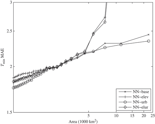
Figure 1 illustrates the performance of the group of models based on the NN interpolator for predicting the minimum daily air temperature. This figure shows that for very dense (density less than one gauge per 1000-km²) networks, these models perform well with an MAE of around 1.8°C and that the accuracy degrades as the sensor network becomes more sparse. For networks with an average gauge density between one gauge per 750 km² and one gauge per 2000 km², the NN-urb model provided the best performance (MAE = 1.8°C), while the NN-elev provided the worst (MAE = 1.9°C). This difference is quite small, so effectively the models exhibited similar accuracy. For gauge networks with moderate density (one gauge per 2000 km² to 1 gauge per 4000 km²), all four models provided similar accuracy with an MAE of around 2°C. For sparse networks (less than one gauge per 4000 km²), the accuracy of the NN-elev and NN-elur models rapidly degrades as the network becomes more sparse, while the accuracy of the NN-base and NN-urb models plateaus to an MAE of approximately 2.3°C at a density of one gauge per 23,000 km² (which represents a single gauge in the entire state of NJ). For this group of models, the NN-urb model provided the lowest MAE over all network densities.

Figure 1. Mean absolute error of the NN spatial models for forecasting minimum daily air temperature (. The x-axis represents the average area represented by each sensor measurement.

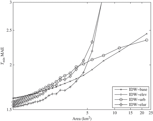
Figure 2 illustrates the performance of the group of models based on the IDW interpolator for predicting the minimum daily air temperature. This figure shows that, for dense networks (density less than one gauge per 1000 km²), all of these models perform well with an MAE of around 1.5°C and that the accuracy degrades as the sensor network becomes sparser. For networks with an average gauge density between one gauge per 750 km² and one gauge per 1000 km², the IDW-base model performs the worst (MAE = 1.6), while the IDW-elev model performs the best (MAE = 1.5). As the gauge density continues to decrease, the IDW-urb model returns slightly less accuracy than the IDW-base model, although the MAE values of the models still remain clustered, with error difference of only 0.1°C. However, for densities less than one gauge per 4000 km², the accuracy of the IDW-elev and IDW-elur models rapidly degrades as the network becomes sparser, while the accuracy of the IDW-base and IDW-urb models continues to rise slowly to an MAE of approximately 2.4°C at a density of one gauge per 23,000 km². For this group of models, the IDW-base model exhibits the best performance for all network densities.

Figure 2. Mean absolute error of the IDW spatial models for forecasting minimum daily air temperature (. The x-axis represents the average area represented by each sensor measurement.

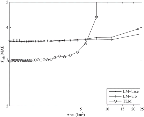
Figure 3 illustrates the performance of the LM and TLM models, which are based on remotely sensed T_LS . This figure shows that for gauge networks with a density less than about one gauge per 4000 km², the LM-base and LM-cs models exhibit an MAE of 3.6°C, whereas the TLM model exhibits an MAE of 3.0. However, as the gauge density decreases further, the accuracy of the TLM model rapidly degrades, whereas the MAE of the LM models rises only slightly, to about 3.7°C, with a slight advantage to the LM-urb model. Thus, for this group of models, the TLM model exhibits the best performance for moderate-to-dense networks, while the LM-urb model exhibits the best performance for sparse networks.

Figure 3. Mean absolute error of the remote sensing-based spatial models for forecasting minimum daily air temperature (. The x-axis represents the average area represented by each sensor measurement.

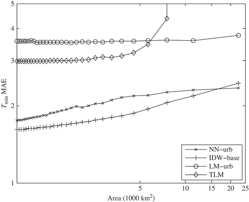
Figure 4 illustrates the performance of the best performing models from each model group. From this figure, it can be clearly seen that the models based on NN and IDW interpolation perform much better over all of the sensor networks examined in this study, with a maximal MAE of 2.4°C for both the NN-urb and IDW-base models. On the other hand, the remote sensing-based spatial models returned an MAE between 3°C and 3.8°C under the best conditions.

Figure 4. Mean absolute error of best performing models for minimum daily air temperature ( from each model group. The x-axis represents the average area represented by each sensor measurement.

Maximum daily air temperature

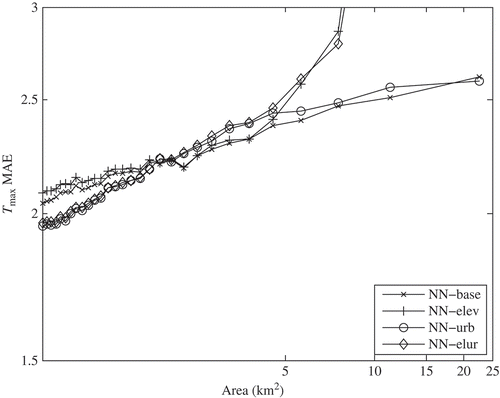
Figure 5 illustrates the performance of the group of models based on the NN interpolator for predicting the maximum daily air temperature. This figure shows that for very dense (density less than one gauge per 1000 km²) networks, these models perform well with an MAE of around 1.8°C and that the accuracy degrades as the sensor network becomes sparser. For networks with an average gauge density between one gauge per 750 km² and one gauge per 2000 km², the NN-urb and NN-elur models provide the best performance (MAE = 1.8°C), while the NN-elev provides the worst (MAE = 1.9°C); again, the difference in MAE is small (0.1°C). For gauge networks with moderate density (one gauge per 2000 km² to one gauge per 4000 km²), all four models provide similar accuracy, with an MAE of about 2.3°C, although NN-base and NN-elev perform slightly better than NN-urb and NN-elur. For sparse networks (less than one gauge per 4000 km²), the accuracy of the NN-elev and NN-elur models rapidly degrades as the network becomes sparser, while the accuracy of the NN-base and NN-urb models rises gently to an MAE of approximately 2.6°C at a density of one gauge per 23,000 km². For this group of models, the NN-urb model provides the lowest MAE over all network densities.

Figure 5. Mean absolute error of the NN spatial models for forecasting maximum daily air temperature (. The x-axis represents the average area represented by each sensor measurement.

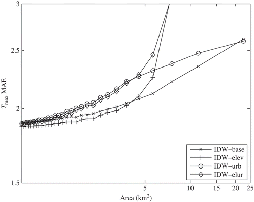
Figure 6 illustrates the performance of the group of models based on the IDW interpolator for predicting the maximum daily air temperature. This figure shows that for dense networks (density less than one gauge per 1000 km²), all of these models perform well, with an MAE of around 1.8°C and that the accuracy degrades as the sensor network becomes sparser. For networks with an average gauge density less than one gauge per 4000 km², the IDW-elev and IDW-base models perform the best (MAE = 1.9°C), although the IDW-elev model is slightly better. In this same range, the IDW-urb model exhibits the largest MAE, 2.0°C; however, the difference in MAE for all four models is within 0.1°C. For gauge networks with a density greater than one gauge per 4000 km², the performance of the two models relying on the environmental lapse rate (IDW-elev and IDW-elur) degrades rapidly, while the MAE of the IDW-base and IDW-urb models continues to rise steadily to 2.6°C for networks of one gauge per 24,000 km². Of the IDW models, the IDW-base exhibits the best performance over the networks explored in this study.

Figure 6. Mean absolute error of the IDW spatial models for forecasting maximum daily air temperature (. The x-axis represents the average area represented by each sensor measurement.

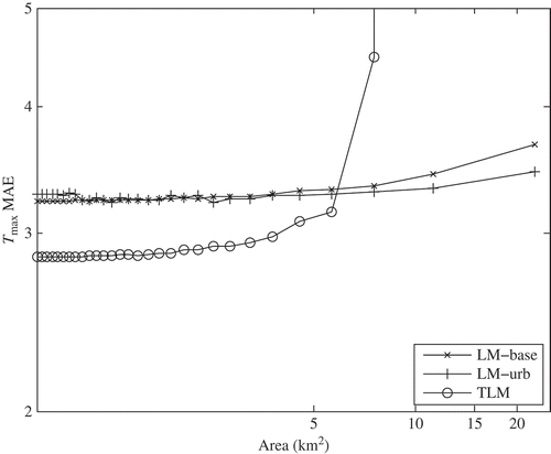
Figure 7 illustrates the performance of the LM and TLM models, which are based on remotely sensed T_LS . This figure shows that for gauge networks with a density less than about one gauge per 4000 km², the LM-base and LM-cs models exhibit an MAE of 3.2°C, whereas the TLM model exhibits an MAE of 2.8. However, as the gauge density decreases further, the accuracy of the TLM model rapidly degrades, whereas the MAE of the LM models rises only slightly, to about 3.7°C, with a slight advantage to the LM-urb model. Thus, for this group of models, the TLM model exhibits the best performance for moderate-to-dense networks, while the LM-urb model exhibits the best performance for sparse networks.

Figure 7. Mean absolute error of the remote sensing–based spatial models for forecasting maximum daily air temperature (. The x-axis represents the average area represented by each sensor measurement.

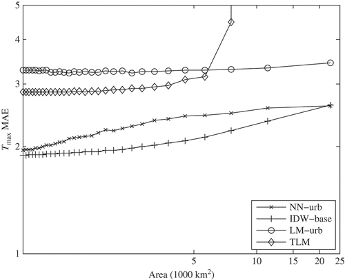
Figure 8 illustrates the performance of the best performing models from each model group. From this figure, it can be clearly seen that the models based on NN and IDW interpolation perform much better over all of the sensor networks examined in this study, with a maximal MAE of 2.6°C for both the NN-urb and IDW-base models. On the other hand, the remote sensing-based spatial models returned an MAE between 2.8°C and 3.4°C under the best conditions.

Figure 8. Mean absolute error of best performing models for maximum daily air temperature ( from each model group. The x-axis represents the average area represented by each sensor measurement.

Discussion

The performance of the 11 models explored in this study was similar for both the minimum and maximum T_A . The NN- and IDW-based models exhibited a lower MAE on the minimum daily T_A data than they did on the maximum daily T_A data. This pattern was reversed for the LM and TLM models, where a lower MAE was observed for the maximum daily T_A predictions. However, in both the min and max T_A cases, it was observed that the models based only on proximity models of ground-based measurements (i.e., the NN- and IDW-based models) had a significantly lower (∼1°C) MAE than did the models based on a thematic transformation of remotely sensed measurements (i.e., LM and TLM) for all gauge network densities.

This is a surprising result, since it was expected that, for very sparse networks, the methods based on proximity models would be outperformed by the methods based on remotely sensed measurements. This expectation was based on the logic that, as the gauge network became sparser, the distance between an ungauged location and its nearest neighboring gauge location would increase. Since spatial proximity is often equated with representativeness, in sparse networks, the nearest gauged locations would not represent the ungauged locations well. This pattern was indeed observed, since the NN and IDW methods' MAEs monotonically increased as the gauge density decreased. However, at the limit of the study region size (22,600 km²), a network consisting of one randomly placed gauge measured a min and max air temperature that is more similar to the min and max air temperature experienced throughout the 22,600 km² study region than is the prediction of the min/max air temperature made using remotely sensed land surface temperature.

Using a proximity-based interpolation model that accounts for land-use similarity (i.e., urbanization) appears to be beneficial for very dense networks. However, since these models use only the measurements from similar urbanization contexts for prediction of an ungauged location, each prediction is based on a subnetwork with a gauge density less than the density of the full network. As the gauge network becomes less dense in general, the benefit gained from using measurements more representative of the urbanization level of the ungauged site is overwhelmed by the detriment of having to go further away to find those gauges. This point occurs at a density of about one gauge per 1000 km² in the NJ study region, and it represents the tradeoff point at which land-use similarity becomes less important to the prediction than proximity. This same tradeoff occurs with the IDW methods as well; however, the proximity benefit appears to be more important for moderately sparse gauge densities (one gauge per 1000 km² to one gauge per 10,000 km²), since the IDW-urb model exhibits a higher MAE than the IDW-base model in this regime by about 0.2°C.

Using an elevation correction improved the IDW models of dense networks, but not the NN models for similarly dense networks. This is probably because the IDW model incorporates measurements from the entire gauge network, whereas the NN model only uses the most proximal measurement. Since gauges located far from the location being estimated may differ greatly in elevation, normalizing all measurements to a constant elevation is more important to the model that includes these distant gauge locations in its prediction than it is to the model that excludes these distant gauge locations. Again, as proximity of the NN decreases, the benefit gained from using an elevation correction increases. However, the elevation-corrected NN and IDW models begin to deteriorate rapidly for gauge networks of approximately one gauge per 4000 km². In the study area, this equates to five gauges in the entire region, a sample size insufficient to produce a representative model (Equation (3)(2b)) of the elevation trend by regression. The TLM model is also plagued by this problem, since it too relies on a regression model of the temperature as a function of the elevation. If the relationship between T_A and elevation could be estimated in a way that was not dependent on the sensor network being representative of the elevation variation in the study region, then these methods might become useful for sparse networks.

Conclusion

This study investigated the performance of several models suggested in the literature for the creation of gridded spatial data sets of minimum and maximum air temperature. The models investigated ranged from simple proximity-based interpolation models to more complicated models based on relationships between remotely sensed land surface temperature and daily min/max air temperature. The proximity-based interpolation models included four variations of a NN interpolator that included land-use and/or elevation corrections and four variations of an IDW interpolator that included land-use and/or elevation corrections. The remote sensing-based models included two variations of a LM relating min/max T_A to T_LS , one of which included a land-use correction, and a LM of T_A based on T_LS , elevation, and seasonality.

A ground-based network of meteorological stations within the state of NJ was used to create approximately 3000 subnetworks representing a random sample of all of the possible networks of size that could exist within the state. These subnetworks were categorized by the average area associated with each gauge, which is the inverse of the average gauge density. Leave-one-out cross-validation was then used to evaluate the error associated with each of the models for predicting the minimum and maximum daily air temperature at ungauged locations using each of the 3000 subnetworks. The MAE was aggregated across the spatial location of the prediction and network geometry, resulting in a curve illustrating the trend in the MAE associated with each model as the gauge network became sparser. These trends were analyzed to reveal that, as the network becomes sparser, the simpler models such as NN or IDW interpolation of the gauge observations (NN-urb and IDW-base) are more reliable than the more complicated models, particularly those models that relied on elevation correction. This result was caused by insufficient representation of the variety of elevations that are present in the study region by the sample of gauges comprising the network. More surprising, however, was the result that, even for very sparse gauge networks consisting of a single ground-based gauge located randomly within the study region of 22,600 km², NN and IDW approaches had significantly (∼1°C) lower MAEs than any of the remote sensing-based models (LM and TLM) – a result that suggests that error inherent in the conversion of land surface temperature to minimum or maximum daily air temperature is more significant than the error inherent in extrapolating minimum or maximum daily air temperature to distances in excess of 80 km in all directions.

To investigate the point at which the LM and TLM models become more appropriate for spatial modeling of min/max T_A than NN or IDW, a much larger study region would need to be investigated. Since a gauge density of one gauge per 22,600 km² is equivalent to a gauge network where the inter-gauge spacing is 84 km, it appears from this study that NN or IDW should be used to created gridded data sets of min/max T_A in cases where the gauges are separated by 84 km or less, though no conclusions can be drawn for networks of gauges with larger separation distances. Additionally, it should also be noted that this study explored a geographical region that is heavily urbanized and that elevations in the study region vary from sea level to 550 m above mean sea level. Thus, the results observed here may not be applicable to regions with lower levels of urbanization or greater elevation variations.

References

- Burt , J. E. , Barber , G. M. and Rigby , D. L. 2009 . Elementary Statistics for Geographers , 3rd ed. , New York : Guilford Press .
- Cresswell , M. P. , Morse , A. P. , Thompson , M. C. and Connor , S. J. 1999 . Estimating Surface Air Temperatures, from Meteosat Land Surface Temperatures, Using an Empirical Solar Zenith Angle Model.” . International Journal of Remote Sensing , 20 ( 6 ) : 1125 – 1132 .
- Dodson , R. and Marks , D. 1997 . Daily Air Temperature Interpolated at High Spatial Resolution over a Large Mountainous Region.” . Climate Research , 8 : 1 – 20 . doi: 10.3354/cr008001.
- Duda , R. O. , Hart , P. E. and Stork , D. G. 2001 . Pattern Classification , New York : Wiley-Interscience .
- Funk , C. , Michaelsen , J. , Verdin , J. , Artan , G. , Husak , G. , Senay , G. , Gadain , H. and Magadazire , T. 2003 . The Collaborative Historical African Rainfall Models: Description and Evaluation.” . International Journal of Climatology , 23 ( 1 ) : 47 – 66 .
- Garen , D. C. and Marks , D. 2005 . Spatially Distributed Energy Balance Snowmelt Modeling in a Mountainous River Basin: Estimation of Meteorological Inputs and Verification of Model Results.” . Journal of Hydrology , 315 ( 1–4 ) : 126 – 153 . doi: 10.1016/j.jhydrol.2005.03.026.
- Hasenauer , H. , Merganicova , K. , Petritsch , R. , Pietsch , S. and Thornton , P. 2003 . Validating Daily Climate Interpolation over Complex Terrain in Austria.” . Agricultural and Forest Meteorology , 119 : 87 – 107 .
- Hasse, J. E., and R. G. Lathrop. 2010. Changing Landscapes in the Garden State: Urban Growth and Open Space Loss in New Jersey from 1986 to 2007. Report published by the Rowan Geolab http://gis.rowan.edu/projects/luc/ (http://gis.rowan.edu/projects/luc/) (Accessed: 11 April 2013 ).
- Hill , D. J. “ Evaluation of the Temporal Relationship between Daily Min/Max Air and Land Surface Temperature ” . In International Journal of Remote Sensing forthcoming
- Jarvis , C. H. and Stuart , N. 2000a . A Comparison among Strategies for Interpolating Maximum and Minimum Daily Air Temperatures. The Selection of ‘Guiding’ Topographic and Land Cover Variables.” . Journal of Applied Meteorology , 40 ( 1 ) : 1060 – 1074 .
- Jarvis , C. H. and Stuart , N. 2000b . A Comparison among Strategies for Interpolating Maximum and Minimum Daily Air Temperatures. The Interaction between Number of Guiding Variables and the Type of Interpolation Method.” . Journal of Applied Meteorology , 40 ( 2 ) : 1075 – 1081 .
- Lin , S. , Moore , N. J. , Messina , J. P. , DeVisser , M. H. and Wu , J. 2012 . Evaluation of Estimating Daily Maximum and Minimum Air Temperature with MODIS in East Africa.” . International Journal of Applied Earth Observation and Geoinformation , 18 : 128 – 140 .
- Lundquist , J. D. , Pepin , N. and Rochford , C. 2008 . Automated Algorithm for Mapping Regions of Cold-Air Pooling in 3 Complex Terrains.” . Journal of Geophysical Research , 113 : 1 – 15 .
- Miliaresis , G. and Tsatsaris , A. 2011 . Mapping the Spatial and Temporal Pattern of Day-Night Temperature Difference in Greece from MODIS Imagery.” . GIScience and Remote Sensing , 48 ( 2 ) : 210 – 224 . doi: 10.2747/1548-1603.2.210.
- Mostovoy , G. V. , King , R. L. , Reddy , K. R. , Kakani , V. G. and Filippova , M. G. 2006 . Statistical Estimation of Daily Maximum and Minimum Air Temperatures from MODIS LST Data over the State of Mississippi.” . GIScience and Remote Sensing , 43 ( 1 ) : 78 – 110 .
- Neteler , M. 2005 . Time Series Processing of MODIS Satellite Data for Landscape Epidemiological Applications.” . International Journal of Geoinformatics , 1 ( 1 ) : 133 – 138 .
- Nieto , H. , Aguado , I. , Chuvieco , E. and Sandholt , I. 2010 . Dead Fuel Moisture Estimation with MSG-SEVIRI Data: Retrieval of Meteorological Data for the Calculation of the Equilibrium Moisture Content.” . Agricultural and Forestry Meteorology , 150 ( 7–8 ) : 861 – 870 .
- Nieto , H. , Sandholt , I. , Aguado , I. , Cuvieco , E. and Stisen , S. 2011 . Air Temperature Estimation with MSG-SEVIRI Data: Calibration and Validation of the TVX Algorithm for the Iperian Peninsula.” . Remote Sensing of the Environment , 115 ( 1 ) : 107 – 116 .
- Piper , E. L. , Smit , M. A. , Boote , K. J. and Jones , J. W. 1996 . The Role of Daily Minimum Temperature in Modulating the Development Rate to Flowering in Soybean.” . Field Crop Research , 47 ( 2–3 ) : 211 – 220 .
- Serbin , S. and Kucharik , C. J. 2008 . Spatiotemporal Mapping of Temperature and Precipitation for the Development of a Multidecal Climatic Dataset for Wisconsin.” . Journal of Applied Meteorological and Climatology , 48 : 742 – 757 .
- Shen , S. and Leptoukh , G. G. 2011 . Estimation of Surface Air Temperature over Central and Eastern Eurasia from MODIS Land Surface Temperature.” . Environmental Research Letters , 6 : 045206 doi: 10.1088/1748-9326/6/4/045206.
- Stahl , K. , Moore , R. D. , Floyer , J. A. , Asplin , M. G. and Mckendry , I. G. 2006 . Comparison of Approaches for Spatial Interpolation of Daily Air Temperature in a Large Region with Complex Topography and Highly Variable Station Density.” . Agricultural and Forest Meteorology , 139 : 224 – 236 .
- Strathopoulou , M. , Cartalis , C. and Chrysoulakis , N. 2006 . Using Midday Surface Temperature to Estimate Cooling Degree-Days from NOAA-AVHRR Thermal Infrared Data: An Application for Athens, Greece.” . Solar Energy , 80 ( 4 ) : 414 – 422 .
- Thornton , P. E. , Running , S. E. and White , M. A. 1997 . Generating Surfaces of Daily Meteorological Variables over Large Regions with Complex Terrain.” . Journal of Hydrology , 190 : 214 – 251 .
- Vallet-Coulomb , C. , Legesse , D. , Gasse , F. , Travi , Y. and Chernet , T. 2001 . Lake Evaporation Estimates in Tropical Africa (Lake Ziway, Ethiopia).” . Journal of Hydrology , 245 ( 1–4 ) : 1 – 18 .
- Vancutsem , C. , Ceccato , P. , Dinku , T. and Connor , S. J. 2010 . Evaluation of MODIS Land Surface Temperature Data to Estimate Air Temperature in Different Ecosystems over Africa.” . Remote Sensing of Environment , 114 : 449 – 465 . doi: 10.1016/j.rse.2009.10.002.
- Vogt , J. V. , Viau , A. A. and Paquet , F. 1997 . Mapping Regional Air Temperature Fields Using Satellite-Derived Surface Skin Temperatures.” . International Journal of Climatology , 17 ( 14 ) : 1559 – 1579 .
- Willmott , C. J. and Rowe , C. M. 1985 . Climatology of the Terrestrial Seasonal Water Cycle.” . Journal of Climatology , 5 : 589 – 606 .