Studying urban development and change in the contiguous United States using two scaled measures derived from nighttime lights data and population census

Abstract

We investigated urban development trend in contiguous United States based on metropolitan areas (MAs), using two scaled measurements for 1990, 2000 and 2010. Linear population density (LPD) was used to compare the same MA over time. Population area growth index (PAGI) was adopted to compare different MAs at the same time. We found that (1) DMSP-OLS nighttime stable lights data are effective for delineating extent of developed areas; (2) both measurements show the growth of developed land have slowed from 1990 to 2010; (3) both measurements show clear regional pattern in urban development in contiguous United States.

Keywords:

• contiguous United States
• urban development
• DMSP-OLS nighttime lights
• population census

1. Introduction

Urban population growth and social–economic change have pushed urban areas to expand at a fast rate worldwide in recent decades. Urban areas in the United States have experienced vast transformation since the end of World War II. Over 80% of the United States population is classified as urban (U.S. Census Bureau 2012). The expansion of developed areas results in the loss of prime farmland and forests, increased energy consumption, increased cost of public services and increased threat to public health (Bhatta 2010; Hasse and Lathrop 2003). It is important to understand the urban growth process for better planning and policy decisions.

Remote sensing has been widely used to capture the extent and track the rapid growth of developed areas, for individual cities (Deng et al. 2009; Masek, Lindsay, and Goward 2000; Yang and Lo 2002; Zhang et al. 2002), regions (Li and Yeh 2004; Martinuzzi, Gould, and Gonzalez 2007), and at national and global scales (Imhoff et al. 1997; Small, Pozzi, and Elvidge 2005; Vogelmann et al. 2001). Accurate and detailed mapping of developed areas requires spatial resolution of 5-m pixels or finer (Forster 1985; Jensen and Cowen 1999). However, it is only practical to use moderate- to coarse-resolution data for regional and continental studies. For the contiguous United States, the National Land Cover Database (NLCD, circa 1992, 2001, 2006) is a reliable product that characterizes land cover conditions including developed areas (Fry et al. 2011; Homer et al. 2004; Vogelmann et al. 2001). The NLCD was derived from 30-m pixel Landsat imagery and ancillary data. Each NLCD product was the result of a multi-year project that involved large amount of resources and manpower. Each NLCD data set is about 16 G in size; manipulation and further analysis of the data set is very time consuming - a simple focal statistics can take an hour on an average computer.

For mapping developed areas at continental or global scale, coarse-resolution nighttime lights data of approximately 2.7 km resolution acquired by the Optical Linescan System of the Defense Metrological Satellite Program (DMSP-OLS) (Elvidge et al. 1997a) have become a good alternative. The reported studies involved global investigations of relationship between DMSP-OLS data and developed area (Small, Pozzi, and Elvidge 2005), comparison of urban growth among world regions (Zhang and Seto 2011), urban growth investigation/urban extraction within the United States (Gallo et al. 2004; Imhoff et al. 1997; Sutton 2003) and dynamics of urban expansion in China (Liu et al. 2012). Researchers have also found strong relationship between DMSP-OLS data and urban population or population density (Sutton et al. 1997, 2001), energy consumption (Amaral et al. 2005; Elvidge et al. 1997b; He et al. 2013), GDP and other social–economic parameters (Forbes 2013; Levin and Duke 2012; Ma et al. 2012; Propastin and Kappas 2012). With less than 5 M in size for each annual composite to cover the entire contiguous United States, the DMSP-OLS data set is much more manageable than any effort to investigate developed areas at the continental scale based on 30-m pixel Landsat imagery and its derivatives.

The relationship between urban population and area has been a perennial topic in urban and economic geography. Change in urban population density over time is frequently used to quantify the changing nature of land consumption in urban areas. There is no consensus in a universal definition or measurement of “urban sprawl”; many identify “low density” as one dimension of sprawl (Bhatta, Saraswati, and Bandyopadhyay 2010; Schneider and Woodcock 2008; Wilson et al. 2003). Stewart and Warntz (1958) presented a consistent log-log linear relationship between population and area using census data for the United States and European cities. Sutton (2003) derived a scale-adjusted sprawl index based on a linear relationship between Ln(population) and Ln(area). Because of the natural log (Ln) transformation, the index allowed for a fair comparison between metropolitan areas (MAs) of different sizes (Sutton 2003). Marshall (2007) developed the linear population density (LPD) to describe urban expansion over time. He demonstrated that the LPD has been relatively stable from 1950 to 2000 for urban areas in the United States, while urban population density has changed by more than a factor of two.

It is interesting to note the similarities and differences between the LPD and Sutton’s scale-adjusted sprawl index. They both were built upon the notion of a nonlinear relationship between urban population and area. was developed from A  Pⁿ, a scaling relationship between area and population, where n was found to be around two for urban areas in the United States (Marshall 2007). It was meant to apply in each urban area over time; and it has remained relatively constant over a 50-year time span (Marshall 2007). Sutton’s index was to compare different urban areas of the same time for their degree of deviation from the regression line. Both measures have advantage over the arithmetic population density (P/A) in that the difference in population size of urban areas matters less in comparison, either through time for the same area (LPD) or across space at the same time (Sutton’s index). Both studies fall within a body of knowledge applying scaling relationships to describe the urbanization process, including the well-known Zipf’s Law (Zipf 1949). A recent study found Zipf’s Law applied to the spatial extent of developed area derived from DMSP-OLS stable nighttime lights data (Small et al. 2011).

There is a lack of empirical investigations reported for the overall urban development status and changes in the entire contiguous United States in recent decades. Sutton’s study (2003) presented a one-time view for the early 1990s. There hasn’t been any published update for the last 20 years using data sets of similar resolution and focusing on patterns within the contiguous United States. Marshall (2007) used Urban Areas defined by the US Census, which could underestimate or overestimate developed areas. Reliable and consistent measurement of the extent of developed area for the contiguous United States over decades of time has been a challenge. In this research, we investigated the recent status and change of urban development in 274 MAs within the contiguous United States. Specifically, we adopted two scaled measurements: LPD for longitudinal tracking of the same MAs and population-area growth index (PAGI, a modified Sutton’s index) for latitudinal comparison of the status of different MAs at the same time. We demonstrate a fast and effective approach to extract the extent of developed area using DMSP-OLS nighttime lights data. Urban population data came from Census 1990, 2000 and 2010. In addition, we also analyzed regional patterns within the contiguous United States using the two scaled measurements. We hypothesize that distinguishable regional development patterns that is typically revealed using finer-resolution data can be found using coarse-resolution nighttime lights data. We also hypothesize that using both the LPD and PAGI would give a richer depiction of the process than either indicator alone.

2. Materials and methods

2.1. Study area and data collection

2.1.1. Study area

Our study area included all MAs within the contiguous United States as defined in Census 2000 TIGER/Line® file. The geographic boundaries of MAs were obtained from US Census Bureau. The MAs included both the metropolitan statistical areas (MSAs) and the consolidated metropolitan statistical areas (CMSAs), defined by the Office of Management and Budget (OMB) (U.S. Census Bureau 2000). The MSAs were county-based functional regions with measurable social–economic connections centered on an urbanized area of 50,000 population or more (OMB 2010). CMSAs were large MAs of more than one million. We visually examined the boundaries of MSAs for the three decennial censuses. Little change in boundaries between Census 1990 and 2000 was found. However, some visible change in boundaries occurred between 2000 and 2010. To make the spatial extent consistent for comparison between 1990, 2000 and 2010, the MAs from Census 2000 was selected. In the contiguous United States, there were 274 MAs defined in the 2000 Census data. Since MAs are county-based geographic unit, both developed and undeveloped land exists within the MA boundaries. That is, the extent of developed area is generally smaller than the extent of the MA.

2.1.2. Urban population counts

For the year 2000, urban population counts were directly retrieved from Census 2000 data released for the MAs. To account for the MA boundary change over the years, urban population were retrieved at the smaller block group (BG) level for Census 1990 and 2010, from the National Historical Geographic Information System (NHGIS) (Minnesota Population Center 2012). Then the population counts at the BG level were summarized for each MA.

2.1.3. DMSP-OLS nighttime stable lights data

To extract developed areas within the MAs, nighttime stable lights (NSL) data from 1992 (the earliest) to 2010 in the Version 4 DMSP-OLS nighttime lights time series were collected from the National Geophysical Data Center (NGDC) of National Oceanic and Atmospheric Administration (NOAA 2012). The data set is a grid of 30 arc second pixels, covering the entire globe from 65° S to 75° N in latitude. Digital numbers (DNs) of the DMSP-OLS NSL data range from 1 to 63 for cities, towns and other sites with persistent lighting. A value of 0 represents the background and noise. The data set for each year was an annual composite of DMSP-OLS images collected during the entire year. To produce the annual composite, better quality data from the center half of the swath were used, while features such as sunlit, glare, moonlit, clouds and lighting were excluded (NOAA 2012). Readers are referred to Elvidge et al. (1997a, 1997b) for detailed description of the DMSP-OLS data.

2.1.4. Ancillary data

For use in the calibration of the NSL data and as reference in the process of extracting developed areas, we collected Landsat TM images for selected MAs and downloaded NLCD data for 1992, 2001 and 2006 (the only years this data set was available at the time of this study) from the Multi-Resolution Land Characteristics Consortium web site (MRLC 2012). The NLCD has been considered a reliable product for national-wide land cover conditions in the United States. For more information about the production of the NLCD, refer to Vogelmann et al. (2001), Homer et al. (2004) and Fry et al. (2011).

2.2. Systematic correction of the DMSP-OLS NSL data

Without strict onboard calibration, DMSP-OLS NSL data from different satellites collected in different years were incompatible for direct multi-year comparison (Elvidge et al. 2009; Liu et al. 2012). Six DMSP satellites (F10, F12, F14, F15, F16 and F18) collected data from 1992 to 2010. Inconsistency was found in the DNs of the NSL data set collected by the same satellite in different years or collected by two satellites for the same year. To improve the comparability of the data, we applied intercalibration and inter-annual composition to the DMSP-OLS NSL data covering contiguous United States, as described in Elvidge et al. (2009) and Liu et al. (2012).

2.3. Extraction of developed areas

Using the systematically-corrected NSL data, we extracted developed areas in the contiguous United States for 1992–2010. A variety of thresholding and classification methods have been proposed and applied for extracting developed areas using DMSP-OLS NSL data (Cao et al. 2009; Elvidge et al. 1997a; Imhoff et al. 1997; Liu et al. 2012). The thresholding method with reliable ancillary data has been widely used for its simplicity and relatively high accuracy (Henderson et al. 2003; Milesi et al. 2003). For this study, we used the NLCD data set as reference to find the optimal threshold for each MA for each of the 3 years when the reference NLCD products were available (1992, 2001 and 2006).

The 30 m NLCD 1992, 2001 and 2006 data set were first aggregated into Level I land use categories; then a nearest-neighbor majority resampling scheme was applied to generate the reference data at 1-km pixels. The new 1-km pixel received the land use label of the majority among the 30-m pixels. All Level II “developed” categories were included to represent developed land. Based on the resampling results, we produced one map to represent the developed area in 1-km pixels for 1992, 2001 and 2006, respectively, and used them as reference data for the thresholding of NSL data collected in corresponding years.

For the NSL data of 1992, 2001 and 2006, a threshold was determined for each MA for each year, where the extracted developed areas best matched the reference NLCD data based on Kappa coefficient (Liu et al. 2012). We developed an automated procedure to extract developed areas for 1992, 2001 and 2006. The procedure applied 63 thresholds (values of 1–63) and compared the thresholding results with the NLCD reference for each MA. The threshold that produced the highest Kappa coefficient was found for each MA and the result from that threshold was retained as the developed area for the MA. Table 1 shows the summary of optimal threshold applied. Then for each MA, the optimal threshold found for 1992 was applied to years 1992–1996, the optimal threshold found for 2001 was applied to years 1997–2003 and the optimal threshold found for 2006 was applied to years 2004–2010. Applying the optimal threshold for each year in the data set, developed areas were extracted for each MA in the contiguous United States from 1992 to 2010.

Table 1. Statistics of the optimal thresholds used to extract developed land in all MAs for 1992, 2001 and 2006, using NLCD data of the corresponding years as reference.

	1992	2001	2006
Mean threshold	55	53	55
Median threshold	56	54	57
Min threshold	29	26	32
Max threshold	63	63	62
Majority threshold	59	57	59

2.4. Measuring linear population density (LPD) and population area growth index (PAGI)

There is no one measurement that captures the complete picture of urban development status in any region. As discussed above, the LPD and Sutton’s index are straightforward and can be easily calculated. LPD measures the ratio between population and the square root of area. Over time in the same MA, LPD is expected to be quite consistent while the regular population density changes in much larger terms (Marshall 2007). This consistence over time makes it a better indicator of density change. Relatively small change in LPD would indicate considerable population dispersion over the area. Following Marshall (2007), LPD was calculated as:

(1)

where P indicates urban population and A indicates developed area.

For each of the 274 MAs in the study area, extracted developed land in 1992 (the earliest available year) was used with urban population of 1990 to derive an LPD measurement for the earlier 1990s, referred to as nominal 1990 data hereafter. The urban population of 2000 and 2010 were used with the extracted developed land area in 2000 and 2010, respectively, to calculate the LPD for these 2 years for each MA.

In Sutton’s research (2003), the linear regression model between Ln(urban area) and Ln(urban population) was expressed as Ln(P) = B₀ + B₁*Ln(A). Considering that area expansion was more of the result of urban population growth and migration, we modified it to be:

(2)

where B₀ is a constant and B₁ indicates the slope of the linear relationship.

This linear regression model defined the “growth line”, and the degree of derivation was measured as how far above or below the “growth line” an MA was. Adopting Sutton’s idea, the PAGI was defined as follows in this study:

(3)

where A_extracted represents the developed area extracted from the DMSP-OLS NSL data for an MA, A_predicted represents the predicted developed area based on the linear relationship defined in Equation (2). The PAGI is measured as the percentage of difference between the extracted and predicted developed area. If the extracted developed area is more than the predicted for a certain MA, it would indicate a higher than average population dispersion with a positive PAGI value. Otherwise, less than predicted developed area would indicate a lower than average population dispersion with a negative PAGI value. Using the developed area extracted from the DMSP-OLS NSL data of 1992, 2000 and 2010 and urban population of 1990, 2000 and 2010, respectively, the PAGI measurements were calculated for 1990, 2000 and 2010 for all 274 MAs in the study area.

2.5. Spatial pattern analysis

There are distinguishable regional trend in population growth and migration in the contiguous United States from 1990–2010 (US Census Bureau 2011). This pattern would be reflected in LPD change and PAGI measurements as well and worthwhile to be analyzed. We investigated these measurements to reveal regional patterns of urban development from 1990 to 2010, using global Moran’s I and hot spot analysis. Moran’s I represents the degree of spatial autocorreltation based on the locations and attributes of features (Goodchild 1986). Comparing the expected and actual I index, along with the p value, Moran’s I procedure evaluates if a pattern is clustered, dispersed or random. Hot spot analysis is based on the Getis-Ord Gi* statistics (Getis and Ord 1992), which identifies statistically significant hot and cold spots. One important consideration that affects the results of both Moran’s I and hot spot analysis is the distance threshold. The farthest distance between any pair of the 274 MAs studied was found to be about 352 km. To determine the reasonable threshold distance for the hot spot analysis, global Moran’s I was calculated for LPD and PAGI measurements for 14 threshold distance values. The threshold distance was selected as 352 km, and then from 400 km to 1000 km, in increment of 50 km. Pattern analysis results were all statistically significant at 95% confidence level. Considering the size of contiguous United States and spatial distribution of the MAs and their geographic context, beyond 1000 km was deemed inappropriate. The threshold distance of 500 km was selected. An analysis of p-values resulted from the Moran’s I procedure showed that the spatial pattern was statistically significant at the 95% confidence level or above for all the LPD and PAGI measurements studied. Each MA would have at least one neighbor within a 500 km distance, but not too many neighbors. In addition, this distance represents well the regional geographic context in contiguous United States.

3. Results and discussion

3.1. Developed land extracted from DMSP-OLS NSL data

The optimal thresholds used to extract developed land from DMSP-OLS NSL data in 1992, 2001 and 2006 are presented in Table 1. They were selected so that the extracted developed land had the highest level of agreement with the reference NLCD data of the corresponding year for each of the 274 MAs, measured using Kappa statistics. Higher thresholds are associated with large, densely developed urban areas. The median threshold was 54 or higher. Because of high levels of urban development in the contiguous United States, many MAs required a high threshold. For example for 2006, 64 MAs out of the 274 required a threshold of 60 or higher.

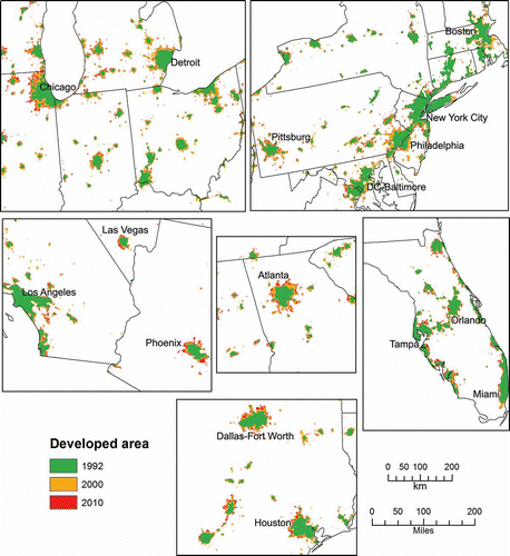
Figure 1 shows the extracted developed land for selected MAs in 1992, 2000 and 2010. Within all MAs, there was a total of 139,909 km² of developed land in 1992, which increased to 227,523 km² in 2000 (an increase of 63.6%), and increased slightly to 239,551 km² in 2010 (5.3% increase). Overall, it indicated that the increase in developed land in the MAs was considerably larger in the 1990s than in the later decade. Similar trend is found in the NLCD data and National Resources Inventory (NRI) report published by the US Department of Agriculture (USDA 2009). Since the NLCD was based on finer-resolution Landsat imagery and NRI report was based on high-resolution aerial survey, they were considered more accurate and can be used as references for results from coarser-resolution imagery such as the NSL data (Cao et al. 2009; Henderson et al. 2003; Liu et al. 2012).

Figure 1. Urban developed land extracted from DMSP/OLS NSL data for selected MAs in the contiguous United States, 1992, 2000 and 2010.

The accuracy of the developed land extraction was evaluated using multiple approaches. The relatively high Kappa statistics indicate high level of agreement with the reference data. For all 274 MAs, both the mean and median Kappa statistics achieved were 0.56 for 1992, 0.52 for 2001 and 0.53 for 2006. The highest Kappa statistics were 0.79 for 1992 and 0.85 for 2001 and 2006. In addition, higher Kappa statistics (>0.7) were associated with large and densely developed MAs in the west, including Los Angeles, San Francisco and Denver. Lower Kappa statistics (< 0.4) were associated with smaller MAs, the majority of which have less than 150,000 urban population in 2010 and located in the northeast. This indicated that the accuracy of the extracted urban area is related to the density of development.

A comparison of total developed area extracted and the NLCD data set is presented in Table 2. Figure 2 shows the overlay of the extraction result and the NLCD reference for areas around Chicago and Los Angeles. The total amount of developed area is highly comparable, and there is also a relatively high spatial agreement between the extracted and reference urban areas. In addition, we conducted an agreement analysis between the extracted developed area and that of the original 30 m NLCD data set, for all 274 MAs in this study. The resultant R² values were found to be between 0.98 and 0.99, with a coefficient close to 1, for 1992, 2001 and 2006. Figure 3 shows the result for 2001. This further indicated that the developed area extracted from systematically corrected DMSP-OLS NSL data at 1-km pixels has a high level of agreement with the NLCD data at 30-m pixels. Landsat TM/ETM+ images of various locations were also used to visually evaluate the results. Many “commission errors” are found where development density is low that is not represented in the NLCD, in which case the extracted developed area from NSL data is a better depiction of the land use. Omission errors are found in linear transportation corridors and small towns where light intensity is low. The accuracy of extracted developed area from NSL data is quite acceptable considering its coarse resolution.

Figure 2. The accuracy of extracted urban developed area from DMSP/OLS NSL data, using NLCD data as reference (Los Angeles and Chicago as examples).

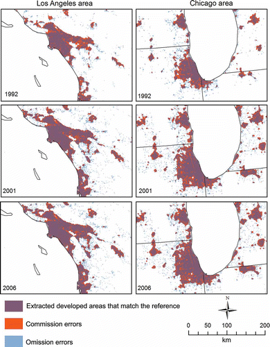
Figure 3. The high agreement between developed area in the original 30 m NLCD 2001 and that extracted from systematically corrected DMSP-OLS NSL data of 2001, for all 274 MAs.

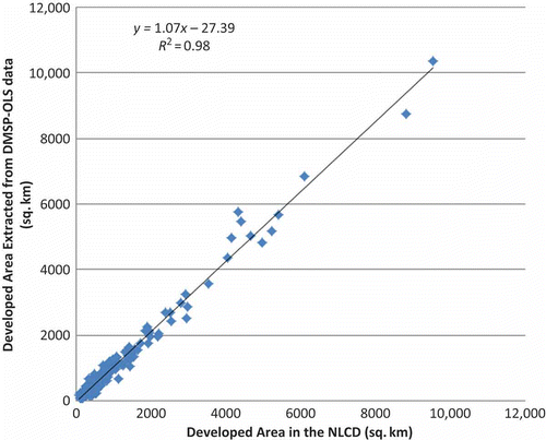
Table 2. A comparison of extracted developed areas from NSL data and the developed areas in NLCD data set for all 274 MAs.

	Extracted developed areas (km^2)	Developed areas in the NLCD (original 30-m pixels) (km^2)	Developed areas in the NLCD (resampled 1-km pixels) (km^2)
1992	139,099	120,381	124,956
2001	227,523	220,464	203,846
2006	239,551	230,431	214,558

3.2. Results based on the LPD measurements

The measured LPD has remained relatively consistent for the MAs between 1990, 2000 and 2010 (Figure 4), as also found by Marshall (2007). In 1990, the 274 MAs had an average LPD of 19.2 persons/m. Average LPD decreased by 1.5 persons/m to 17.7 persons/m in 2000 and then increased by about 1 person/m to 18.7 persons/m in 2010. New York and Los Angeles had the highest LPD in all years, much higher than other MAs. From 1990 to 2000, 22 out of the 274 MAs (including 10 MAs in the largest 50 based on their 2010 population) had a decrease in LPD of 5 persons/m or more, while 10 MAs (eight among the largest 50) had increased LPD of 5 persons/m or more. MAs centered on Las Vegas and Phoenix had the largest LPD increase of 18.6 persons/m and 12.6 persons/m, respectively, indicating significant density increase. A few large MAs in the Midwest (e.g., Detroit, Cleveland, Pittsburg and Chicago), along with Philadelphia, had substantial decrease in LPD during this period. From 2000 to 2010, only New Orleans had a decrease in LPD of 5 persons/m or more and 17 MAs had increased LPD of 5 persons/m or more, including Houston, Dallas-Fort Worth, Washington-Baltimore, Orlando, Los Angeles and Atlanta, in that order. Overall, the measurements of LPD suggested that the outward dispersion of urban population was more of a phenomenon in the 1990s than in the later decade.

Figure 4. The change in linear population density (LPD) for all MAs, 1990–2000 and 2000–2010.

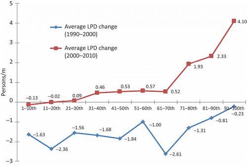
In addition, an analysis of population size of the MAs and the average change in their LPD for all 274 MAs revealed that the larger the MAs in population (top percentiles), the greater the increase in LPD from 2000 to 2010, also the smaller the decrease in LPD from 1990 to 2000 in general (Figure 5). The average in LPD change based on every 10th percentile clearly shows the overall trend of decreased density in the 1990s and increase in the later decade. From 1990 to 2000, all percentile groups have decreased average LPD. The 91–100th percentile (largest 10% in population size) had the smallest decrease. From 2000 to 2010, all percentile groups except the lowest two had increased in average LPD.

Figure 5. The size of urban population and the average change in LPD for all 274 MAs.

3.3. Results based on the PAGI measurements

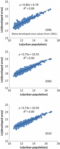
Strong linear relationship between Ln(P) and Ln(A) was found for 1992, 2000 and 2010 based on data for all 274 MAs, with R² around 0.89 (Figure 6). We also noticed that the slope B₁ was 0.86 for 1990, and it decreased to 0.75 for 2000 and 0.73 for 2010. It could be interpreted as that on average, the same amount of population growth in 2000 and 2010 would result in less increase in developed land proportionally. This might be considered a good sign that the land consumption rates have slowed, compared to the early 1990s.

Figure 6. The linear relationship between Ln(urban population) and Ln(developed area).

Spatially, the results show the regional discrepancy of PAGI well. For 1990, 2000 and 2010, many MAs in the South and Midwest had higher than average level of population dispersion. MAs on the eastern coast and in the west consistently had lower than average level of population dispersion (Figure 7), where Sutton’s study (2003) had found lower level of “sprawl”. Table 3 shows that the number of MAs in the “highly dispersed” category where extracted developed area is 30% or more than the predicted area, has decreased from 1990 to 2010. On the other hand, the number of MAs in the “highly compact” category where the predicted area is 30% or more than extracted developed area, has also decreased. Overall, the percentage of derivation above or below the “growth line” has decreased from 1990 to 2010, which indicates the converging of the MAs along the regression line. The largest two MAs, New York and Los-Angeles, consistently had a lower than average PAGI which indicated that they were relatively more compact.

Figure 7. The PAGI measured for all MAs, 1990, 2000 and 2010.

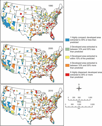
Table 3. Summary of PAGI for all 274 MAs in 1990, 2000 and 2010.

	Number of MAs in each category
PAGI Category	1990	2000	2010
1 Highly compact	64	61	59
2	50	41	39
3	65	60	68
4	55	79	72
5 Highly dispersed	40	33	36

3.4. Results of spatial pattern analysis

The examination of LPD change and PAGI for all MAs in the study area revealed spatial clusters of similar values and regional discrepancies. Results from the Moran’s I and hot spot analysis based on the Getis-Ord Gi* statistics further quantified the observed spatial pattern. Moran’s I values indicated highly clustered pattern for LPD change and PAGI measurements (Table 4). All the I indices are statistically significant at 95% level or above.

Table 4. Moran’s I for LPD change and PAGI measurements.

		Moran’s I	p-value
LPD Change	1990–2000	0.19	<0.001
	2000–2010	0.21	<0.001
PAGI	1990	0.24	<0.001
	2000	0.20	<0.001
	2010	0.18	<0.001

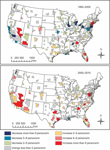
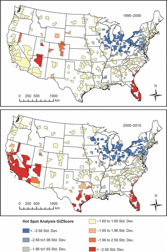
The hot spot analysis visually revealed statistically significant regional clusters. For the change in LPD from 1990 to 2000, the result shows a strong cluster of decreased LPD values in the Midwest and Great Lakes region (Figure 8). On the other hand, a strong cluster of increased LPD values was found in the Florida Peninsula and a secondary cluster around Denver (Figure 7). From 2000 to 2010, statistically significant clusters of positive change are found in the south-western coast region, southern Texas and the Florida Peninsula and clusters of negative change are again found in the Midwest and Great Lakes region (Figure 8). This pattern of LPD change matches the population growth pattern, where the south and west had experienced faster growth.

Figure 8. Hot spot analysis results of LPD change measurements, 1990–2000 and 2000–2010.

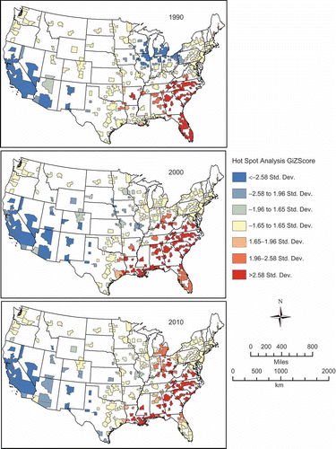
The hot spot analysis of PAGI in 1990, 2000 and 2010 found some similar pattern. For all 3 years, there were statistically significant lower than average PAGI values (more compact) found in the west (Figure 9). Significantly higher than average PAGI values were found in south. Noticeably, a higher than average PAGI cluster emerged in the Midwest from 1990 to 2010, either attribute to depopulation or faster growth in land consumption than population growth.

Figure 9. Hot spot analysis results of PAGI measurements for 1990, 2000 and 2010.

4. Conclusions

We presented an empirical study on urban development status in 1990, 2000 and 2010 and changes between the years, for 274 MAs in the contiguous United States. Two scaled measurements were adopted for that purpose: the LPD – to compare the development status of the same MA overtime; and the PAGI – to compare all the MAs across space at the same time. Both measurements were straight-forward and easy to calculate, and allowed for a relatively fair comparison of MAs of different sizes because of the scaling.

Urban population for the 274 MAs was retrieved from Census 1990, 2000 and 2010. The extent of developed land for 1992, 2000 and 2010 was extracted from calibrated coarse-resolution DMSP-OLS NSL data. The utilization of DMSP-OLS NSL data and the optimal thresholding method made the areal measurement of developed land for all 274 MAs effective, consistent and manageable over the entire contiguous United States for the study period.

The following conclusions can be drawn through the analysis of results:

1. The dispersion of urban population had slowed between 2000 and 2010 compared to the previous decade, as shown in both LPD and PAGI measurements. Density measured by average LPD decreased from 1990 to 2000 but increased from 2000 to 2010. Furthermore, the coefficients (slope) of the linear regression models between Ln(population) and Ln(developed area) decreased from 1990 to 2000 and to 2010, indicating that population growth has resulted in less increase in developed land in the later decade.

2. Compared to 1990, the difference in PAGI among the MAs has decreased in 2000 and 2010. On average, MAs are located closer to the “growth line”, indicating that the MAs have become similar to each other in terms of the level of dispersion.

3. There was a statistically significant clustered pattern in both the PAGI values for the MAs at the same year and the change in LPD over time.

In summary, we found that DMSP-OLS NSL data serve as good proxy for deriving information on the extent of developed areas in the contiguous United States, which made data processing much more manageable. The LPD measurement has been quite consistent for the MAs over time from 1990 to 2010, as was found by Marshall (2007). LPD can be effectively used for the prediction of future needs for urban land according to population projections. A strong correlation existed between Ln(urban population) and Ln(developed area), well supported by the literature for example, in Stewart and Warntz (1958) and Sutton (2003). Combining LPD and PAGI allows a richer depiction of the urban development process.

It is worthwhile to note the uncertainty in using the NSL data to extract urban areas. The relatively coarse spatial and radiometric resolutions of the data and “blooming effect” (Small, Pozzi, and Elvidge 2005) contribute to developed land been slightly exaggerated. The newly available data from the “day-night band” of the Visible Infrared Imaging Radiometer Suite (VIIRS) instrument on the Suomi NPP satellite show finer details of nighttime lights (NASA 2012), which have new potentials in mapping developed areas at regional and global scales with higher accuracy. This study is also constrained by the availability of the DMSP-OLS and NLCD data sets. The earliest DMSP-OLS annual composite is available for 1992. Though it was not 1990, but it would be a close approximation of the urban development condition in 1990. The thresholds for extraction of developed land were derived using NLCD data of 1992, 2001 and 2006, the only years available. The systematic correction of the DMSP-OLS data greatly improved the compatibility of the data set so that the thresholds could be applied to the years immediately before and after the 3 years when NLCD data are available. On the other hand, it shows the strength of our method to work effectively with data sets that have temporal gaps.

This study provided an empirical investigation of the status and trend in urban development in the contiguous United States from 1990 to 2010, at the MA level. Spatial details and patterns within each MA were not studied. In addition, the causes behind the recent change also warrant further research. Whether it was the population migration from the “rust-belt” to the “sun-belt” or the sustainable policies and planning strategies at the local level, or other social–economic factors that had made a difference, are yet to be studied.

Acknowledgements

The research is partially supported by Murray State University, the National Basic Research Program of China (grant number 2010CB950901), and the State Key Laboratory of Earth Surface Processes and Resource Ecology of Beijing Normal University (grant number 2010-KF-02).

References

- Amaral, S., G. Câmara, A. M. V. Monteiro, J. A. Quintanilha, and C. D. Elvidge. 2005. “Estimating Population and Energy Consumption in Brazilian Amazonia Using DMSP Night-Time Satellite Data.” Computers, Environment & Urban Systems 29 (2): 179–195.
- Bhatta, B. 2010. Analysis of Urban Growth and Sprawl from Remote Sensing Data. Berlin: Springer-Verlag.
- Bhatta, B., S. Saraswati, and D. Bandyopadhyay. 2010. “Urban Sprawl Measurement from Remote Sensing Data.” Applied Geography 30 (4): 731–740.
- Cao, X., J. Chen, H. Imura, and O. Higashi. 2009. “A SVM-Based Method to Extract Urban Areas from DMSP-OLS and SPOT VGT Data.” Remote Sensing of Environment 113 (10): 2205–2209.
- Deng, J. S., K. Wang, H. Yang, and J. G. Qi. 2009. “Spatio-Temporal Dynamics and Evolution of Land Use Change and Landscape Pattern in Response to Rapid Urbanization.” Landscape and Urban Planning 92 (3–4): 187–198.
- Elvidge, C. D., K. E. Baugh, E. A. Kihn, H. W. Kroehl, and E. R. Davis. 1997a. “Mapping of City Lights Using DMSP Operational Linescan System Data.” Photogrammetric Engineering and Remote Sensing 63 (6): 727–734.
- Elvidge, C. D., K. E. Baugh, E. A. Kihn, H. W. Kroehl, E. R. Davis, and C. Davis. 1997b. “Relation between Satellite Observed Visible – Near Infrared Emissions, Population, and Energy Consumption.” International Journal of Remote Sensing 18 (6): 1373–1379.
- Elvidge, C. D., D. Ziskin, K. E. Baugh, B. T. Tuttle, T. Ghosh, D. W. Pack, E. H. Erwin, and M. Zhizhin 2009. “A Fifteen Year Record of Global Natural Gas Flaring Derived from Satellite Data.” Energies 2 (3): 595–622.
- Forbes, D. J. 2013. “Multi-Scale Analysis of the Relationship between Economic Statistics and DMSP-OLS Night Light Images.” GIScience & Remote Sensing 50 (5): 483–499.
- Forster, B. 1985. “An Examination of Some Problems and Solutions in Monitoring Urban Areas from Satellite Platforms.” International Journal of Remote Sensing 6 (1): 139–151.
- Fry, J., G. Xian, S. Jin, J. Dewitz, C. Homer, L. Yang, C. Barnes, N. Herold, and J. Wickham. 2011. “Completion of the 2006 National Land Cover Database for the Conterminous United States.” Photogrammetric Engineering and Remote Sensing 77 (9): 858–864.
- Gallo, K. P., C. D. Elvidge, L. Yang, and B. C. Reed. 2004. “Trends in Night-Time City Lights and Vegetation Indices Associated with Urbanization Within the Conterminous USA.” International Journal of Remote Sensing 25 (10): 2003–2007.
- Getis, A., and J. K. Ord. 1992. “The Analysis of Spatial Association by Use of Distance Statistics.” Geographical Analysis 24 (3): 189–206.
- Goodchild, M. F. 1986. Spatial Autocorrelation. CATMOG 47. Accessed August 2, 2013. http://qmrg.org.uk/files/2008/11/47-spatial-aurocorrelation.pdf
- Hasse, J. E., and R. G. Lathrop. 2003. “Land Resource Impact Indicators of Urban Sprawl.” Applied Geography 23 (2–3): 159–175.
- He, C., Q. Ma, Z. Liu, and Q. Zhang. 2013. “Modeling the Spatiotemporal Dynamics of Electric Power Consumption in Mainland China Using Saturation-Corrected DMSP/OLS Nighttime Stable Light Data.” International Journal of Digital Earth. doi:10.1080/17538947.2013.822026.
- Henderson, M., E. T. Yeh, P. Gong, C. D. Elvidge, and K. E. Baugh. 2003. “Validation of Urban Boundaries Derived from Global Night-Time Satellite Imagery.” International Journal of Remote Sensing 24 (3): 595–609.
- Homer, C., C. Huang, L. Yang, B. Wylie, and M. Coan. 2004. “Development of a 2001 National Land Cover Database for the United States.” Photogrammetric Engineering and Remote Sensing 70 (7): 829–840.
- Imhoff, M. L., W. T. Lawrence, D. C. Stutzer, and C. D. Elvidge. 1997. “A Technique for Using Composite DMSP/OLS ‘City Lights’ Satellite Data to Accurately Map Urban Areas.” Remote Sensing of Environment 61 (3): 361–370.
- Jensen, J. R., and D. C. Cowen. 1999. “Remote Sensing of Urban/Suburban Infrastructure and Socio-Economic Attributes.” Photogrammetric Engineering and Remote Sensing 65 (5): 611–622.
- Levin, N., and Y. Duke. 2012. “High Spatial Resolution Night-Time Light Images for Demographic and Socio-Economic Studies.” Remote Sensing of Environment 119: 1–10.
- Li, X., and A. G. O. Yeh. 2004. “Analyzing Spatial Restructuring of Land Use Patterns in a Fast Growing Region Using Remote Sensing and GIS.” Landscape and Urban Planning 69 (4): 335–354.
- Liu, Z., C. He, Q. Zhang, Q. Huang, and Y. Yang. 2012. “Extracting the Dynamics of Urban Expansion in China Using DMSP-OLS Nighttime Light Data from 1992 to 2008.” Landscape and Urban Planning 106 (1): 62–72.
- Ma, T., C. Zhou, T. Pei, S. Haynie, and J. Fan. 2012. “Quantitative Estimation of Urbanization Dynamics Using Time Series of DMSP/OLS Nighttime Light Data: A Comparative Case Study from China’s Cities.” Remote Sensing of Environment 124: 99–107.
- Marshall, J. D. 2007. “Urban Land Area and Population Growth: A New Scaling Relationship for Metropolitan Expansion.” Urban Studies 44 (10): 1889–1904.
- Martinuzzi, S., W. A. Gould, and O. M. R. Gonzalez. 2007. “Land Development, Land Use, and Urban Sprawl in Puerto Rico Integrating Remote Sensing and Population Census Data.” Landscape and Urban Planning 79 (3–4): 288–297.
- Masek, J. G., F. E. Lindsay, and S. N. Goward. 2000. “Dynamics of Urban Growth in the Washington DC Metropolitan Area, 1973–1996, from Landsat Observations.” International Journal of Remote Sensing 21 (18): 3473–3486.
- Milesi, C., C. D. Elvidge, R. R. Nemani, and S. W. Running. 2003. “Assessing the Impact of Urban Land Development on Net Primary Productivity in the Southeastern United States.” Remote Sensing of Environment 86 (3): 401–410.
- Minnesota Population Center. 2012. National Historical Geographic Information System: Version 2.0. Minneapolis: University of Minnesota.
- MRLC. 2012. “National Land Cover Database (NLCD).” Accessed August 2, 2013. http://www.mrlc.gov/
- NASA. 2012. “Earth at Night 2012.” Accessed August 2, 2013. http://earthobservatory.nasa.gov/Features/NightLights/?src=features-recent
- NOAA. 2012. “Version 4 DMSP-OLS Nighttime Lights Time Series.” Accessed August 2, 2013. http://ngdc.noaa.gov/eog/dmsp/downloadV4composites.html
- Office of Management and Budget (OMB). 2010. “2010 Standards for Delineating Metropolitan and Micropolitan Statistical Areas.” Federal Register, Vol. 75, No. 123. June 28, 2010/Notices. Accessed August 2, 2013. http://www.whitehouse.gov/sites/default/files/omb/assets/fedreg_2010/06282010_metro_standards-Complete.pdf
- Propastin, P., and M. Kappas. 2012. “Assessing Satellite-Observed Nighttime Lights for Monitoring Socioeconomic Parameters in the Republic of Kazakhstan.” GIScience & Remote Sensing 49 (4): 538–557.
- Schneider, A., and C. E. Woodcock. 2008. “Compact, Dispersed, Fragmented, Extensive? A Comparison of Urban Growth in Twenty-Five Global Cities Using Remotely Sensed Data, Pattern Metrics and Census Information.” Urban Studies 45 (3): 659–692.
- Small, C., C. D. Elvidge, D. Balk, and M. Montgomery. 2011. “Spatial Scaling of Stable Night Lights.” Remote Sensing of Environment 115 (2): 269–280.
- Small, C., F. Pozzi, and C. D. Elvidge. 2005. “Spatial Analysis of Global Urban Extent from DMSP-OLS Night Lights.” Remote Sensing of Environment 96 (3–4): 277–291.
- Stewart, J. Q., and W. Warntz. 1958. “Physics of Population Distribution.” Journal of Regional Science 1 (1): 99–121.
- Sutton, P., D. Roberts, C. Elvidge, and K. Baugh. 2001. “Census from Heaven: An Estimate of the Global Human Population Using Night-Time Satellite Imagery.” International Journal of Remote Sensing 22 (16): 3061–3076.
- Sutton, P., C. Roberts, C. Elvidge, and H. Meij. 1997. “A Comparison of Nighttime Satellite Imagery and Population Density for the Continental United States.” Photogrammetric Engineering and Remote Sensing 63 (11): 1303–1313.
- Sutton, P. C. 2003. “A Scale-Adjusted Measure of ‘Urban Sprawl’ Using Nighttime Satellite Imagery.” Remote Sensing of Environment 86 (3): 353–369.
- U.S. Census Bureau. 2000. “Census 2000 TIGER/Line® Files Technical Documentation.” Accessed August 2, 2013. http://www2.census.gov/geo/tiger/tiger2k/tiger2k.pdf
- U.S. Census Bureau. 2011. “Population distribution and change: 2000 to 2010. 2010 Census Briefs.” Accessed August 9, 2013. http://www.census.gov/prod/cen2010/briefs/c2010br-01.pdf
- U.S. Census Bureau. 2012. “Growth in Urban Population Outpaces Rest of Nation, Census Bureau Reports.” Accessed August 2, 2013. http://www.census.gov/newsroom/releases/archives/2010_census/cb12-50.html
- U.S. Department of Agriculture (USDA). 2009. Summary Report: 2007 National Resources Inventory, Natural Resources Conservation Service, Washington, DC, and Center for Survey Statistics and Methodology, 123p. Ames: Iowa State University. Accessed August 2, 2013. http://www.nrcs.usda.gov/Internet/FSE_DOCUMENTS/stelprdb1041379.pdf
- Vogelmann, J. E., S. M. Howard, L. Yang, C. R. Larson, B. K. Wylie, and N. Van Driel. 2001. “Completion of the 1990’s National Land Cover Data Set for the Conterminous United States from Landsat Thematic Mapper Data and Ancillary Data Sources.” Photogrammetric Engineering and Remote Sensing 67 (6): 650–662.
- Wilson, E. H., J. D. Hurd, D. L. Civco, M. P. Prisloe, and C. Arnold. 2003. “Development of a Geospatial Model to Quantify, Describe and Map Urban Growth.” Remote Sensing of Environment 86 (3): 275–285.
- Yang, X., and C. P. Lo. 2002. “Using a Time Series of Satellite Imagery to Detect Land Use and Land Cover Changes in the Atlanta, Georgia Metropolitan Area.” International Journal of Remote Sensing 23 (9): 1775–1798.
- Zhang, Q., and K. C. Seto. 2011. “Mapping Urbanization Dynamics at Regional and Global Scales Using Multi-Temporal DMSP/OLS Nighttime Light Data.” Remote Sensing of Environment 115 (9): 2320–2329.
- Zhang, Q., J. Wang, X. Peng, P. Gong, and P. Shi. 2002. “Urban Built-up Land Change Detection with Road Density and Spectral Information from Multi-Temporal Landsat TM Data.” International Journal of Remote Sensing 23 (15): 3057–3078.
- Zipf, G. K. 1949. Human Behavior and the Principle of Least-Effort. Cambridge, MA: Addison-Wesley.