Estimation of sea ice thickness in the Bohai Sea using a combination of VIS/NIR and SAR images

Abstract

The thicknesses of level and rough sea ice in the Bohai Sea were estimated, using Huan Jing-1 (HJ-1) charge-coupled device (CCD) images and environmental satellite (ENVISAT) advanced synthetic aperture radar (ASAR) images, respectively. Two empirical models were developed, one to describe the relationship between the reflectance of visible/near-infrared (VIS/NIR) imagery and level ice thickness and one to describe the relationship between the backscattering coefficient of synthetic aperture radar (SAR) imagery and rough ice thickness. The results showed that the VIS/NIR images were more suitable for distinguishing sea ice from sea water, and the active microwave remote sensing images were suitable for determining the difference between level and rough sea ice. The thickness of the level sea ice was logarithmically related to the VIS/NIR reflectance, and the R² value of the fitted curve was 0.99 with a root mean square error (RMSE) of 1.0 cm. In contrast, the thickness of the rough sea ice was exponentially related to the SAR backscattering coefficient, and the R² value of the fitted curve was 0.90 with an RMSE of 2.3 cm. The thicknesses of level and rough sea ice were then calculated using the empirical models, and the results reflected the thickness distribution of sea ice in the Bohai Sea. We concluded that high-resolution images can accurately extract the sea ice area and estimate the thickness of sea ice.

Keywords:

• sea ice
• Bohai Sea
• SAR
• VIS/NIR
• empirical model

1. Introduction

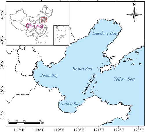
The Bohai Sea is a nearly closed and shallow sea within the mainland of China. The coastline is basically triangular, with three protruding angles corresponding to Liaodong Bay, Bohai Bay and Laizhou Bay (Feng, Li, and Li 1999), as shown in Figure 1. The first-year ice is found in the Bohai Sea from November to the following March. The thickness of the sea ice in Bohai is less than 1 m in most areas, but the ice that accumulates on the shore can reach up to several metres in thickness (Ding 1999). As the most important economic zone in northern China, the marine gross product of the Bohai Sea Rim is 1.6442 trillion yuan, accounting for 36.1% of the national marine gross product (State Oceanic Administration People’s Republic of China 2012). The sea ice causes considerable damage to the marine transportation and aquaculture industries, as well as offshore oil platforms every year (Deng 1986). Therefore, knowledge of the distribution and thickness of the sea ice is extremely important for understanding the mechanism of atmosphere–sea heat exchange, sea ice engineering, marine transportation, marine aquaculture, sea ice disaster prevention and reduction and sea ice resource utilization in the Bohai Sea (Xie et al. 2002; Yang 2000; Guo et al. 2008; Gu et al. 2012).

Figure 1. The location of the Bohai Sea. For full colour versions of the figures in this paper, please see the online version.

Satellite remote sensing technology can be used to obtain rapid access to the reflection of electromagnetic waves and radiation or scattering images of the Bohai Sea ice over large areas. These images can be used to further estimate or predict the properties of the sea ice, such as the area, thickness and surface roughness. Guo, Zhao, and Wang (2000) used microwave (λ = 0.8, 5, 10, 21 cm) measurements of the sea ice thickness to derive an automatic method to estimate the sea ice thickness using a microwave radiometer, and an exponential model was used to describe the relationship between ice thickness and brightness temperature. Yang (2000) proposed an exponential model to describe the relationship between the sea ice thickness and the reflectance at the second band (0.725–1.0 μm) and the brightness temperature at the fourth band (10.3–11.3 μm) of National Oceanic and Atmospheric Administration 14 (NOAA 14) images (bands 1 and 2 correspond to 0.55–0.68 μm and 0.725–1.1 μm, respectively). This model can be used to estimate the thickness of sea ice. Xie et al. (2003) proposed a method to estimate the sea ice thickness using NOAA 17 images (bands 1 and 2 correspond to 0.58–0.68 μm and 0.725–1.1 μm, respectively) based on the theory of short-wave solar radiation. This method can be used to describe the normalized relationship between the reflectance and thickness of sea ice based on a logarithmic model. The sea ice reflectance was normalized relative to the sea water reflectance and the maximum sea ice reflectance. Luo et al. (2005) proposed a piecewise linear estimation model of the sea ice thickness based on the use of Hai Yang-1 (HY-1) images (bands 6 and 7 correspond 0.66–0.68 μm and 0.73–0.77 μm, respectively). Wu, Xu, and Hao (2005) and Wu et al. (2006) proposed a linear model and a piecewise linear model, respectively, to estimate the sea ice thickness using moderate resolution imaging spectroradiometer (MODIS) remote sensing images. Ning et al. (2009) differentiated the sea ice type using band 4 (0.545–0.564 μm) of MODIS images and then estimated the sea ice thickness according to the classification results. Zhang (2011) derived the body scattering component by decomposing the polarimetric Radar satellite-2 (Radarsat-2) images (C-band) to estimate the thickness of the sea ice. For the first-year ice in other seas, some researchers have suggested other methods for the estimation of the sea ice thickness. The Finnish Meteorological Institute (FMI) published operational ice thickness charts based on synthetic aperture radar (SAR; C-band) and icebreaker data with 500 m resolution, and the ice thickness charts were delivered to ships and updated to the Internet (Finnish Meteorological Institute 2014). The Finnish Ice Service (FIS) produced an estimate of the Baltic Sea ice thickness based on a thermodynamic ice model (high-resolution thermodynamic snow/ice model, HIGHTSI) and SAR data for navigation (Karvonen, Cheng, and Similä 2007; Karvonen et al. 2008). Nakamura et al. (2009) and other scholars proposed that the ratio of vertical vertical (VV) to horizontal horizontal (HH) (C-band) is more closely related to the salinity and thickness of sea ice, and the salinity is closely related to the thickness. The authors proposed an empirical model for estimating sea ice thickness that was suitable for Lützow-Holm Bay. The model estimated the sea ice thickness according to the VV/HH ratio. Similä et al. (2010) estimated the thickness of sea ice in the Baltic Sea by combining the MODIS night-time (thermal infrared band) data with ENVISAT advanced synthetic aperture radar (ASAR) images (C-band) to estimate the thickness of level sea ice based on the ice surface temperature derived from MODIS and a one-dimensional thermodynamic model. The authors then estimated the thickness of the rough sea ice using the ENVISAT ASAR images (C-band) and the empirical model, which described the thickness and backscattering coefficient of the sea ice. Toyota et al. (2011) proposed an empirical model of the relationship between the sea ice thickness and the backscattering coefficient of the L-band in the Okhotsk Sea area.

A precise physical radiative transfer model can be better developed using the reflection, radiation and scattering of the electromagnetic waves from sea ice (Grenfell and Perovich 1981; Grenfell 1983; Stogryn and Desargant 1985; Ulaby, Moore, and Fung 1986; Campbell and Wynne 2011; Filippi et al. 2012). However, a physical model requires the input of several parameters and information on the icy conditions of the sea ice, such as the percentage of sea ice brine pockets, the percentage of bubbles, the ice structure and the freezing temperature of sea ice. Due to the current inability to obtain additional remote sensing data regarding the surface features, an empirical or semi-empirical model is a good choice. Compared with the existing methods and models for the estimation of sea ice thickness, methods using visible/near-infrared (VIS/NIR) remote sensing images exhibit the least uncertainty (Yuan et al. 2012; Liu et al. 2013). According to the radiative transfer and scattering theory (Tsang, Kong, and Ding 2004), the reflectance from the VIS/NIR bands is less sensitive to measuring the thickness of rough sea ice. Level sea ice reflects the microwaves easily, and the echo energy from the backscattering direction is low; therefore, this parameter is not useful to determine the thickness of level sea ice, although it can be used to measure rough sea ice thickness. In addition, the thickness and roughness of the first-year sea ice are relatively strongly correlated according to Toyota et al. (2011). It can be seen that different band images are suitable for different uses, especially the integration of VIS/NIR remote sensing images and active microwave remote sensing images (Sheorana and Haackb 2013; Pereira, Freitas, and Siqueira St Anna 2013). Therefore, we propose a method that involves the combination of Huan Jing-1 (HJ-1) charge-coupled device (CCD) images (VIS/NIR remote sensing images) to estimate the thickness of level sea ice and ENVISAT ASAR images (active microwave remote sensing images) to estimate the thickness of rough sea ice.

2. Data and methods

2.1. Data sources

The HJ-1 (A/B) satellite was launched in September 2008 and is comanaged and operated by the China National Committee for Disaster Reduction and the Ministry of Environmental Protection. The HJ-1A is equipped with a CCD camera and Hyperspectral Imager (HSI), and the HJ-1B is equipped with a CCD camera and an IRS (infrared sensor) (China Center for Resources Satellite Data and Application 2009). The images used in this article were acquired by the CCD camera equipped on the HJ-1B satellite on 14 February 2011 03:04:23 am UTC (Universal Time Coordinated). The surface spatial resolution of the images is 30 m, and the swath width is 360 km. The specific parameters are shown in Table 1. The solar elevation angle was 33.81°, with an azimuth angle of 343.30°. The geographic coordinates of the image centre were 119.7230°E, 41.3355°N (see Figure 1).

Table 1. The parameters of the HJ-1 CCD.

Band number	Wavelength (μm)	Revisit period
1	0.43–0.52	4 days
2	0.52–0.60
3	0.63–0.69
4	0.76–0.90

The ENVISAT satellite was launched by the European Space Agency (ESA) in 2002. The imaging waveband of the ASAR carried in the satellite is a C-band, which can image via multipolarization and cross polarization, and there are five multipolarization models (VV, HH, VV/HH, HV/HH and VH/VV) (European Space Agency 2002). The ASAR images used were VV polarization WS (Wide Swath) images. The acquisition time of the images was 14 February 2011 02:02:59 am UTC, the imaging swath was approximately 400 km, the resample resolution (cubic convolution) was 75 m (the original resolution was 150 m), and the geographic coordinates of the imaging centre were 122.018°E, 39.0429°N (Track: 276, Row: 2788), with a 30.76° (19–40°) incidence angle at the centre as shown in Figure 2. Although there is a difference in acquisition time of a little more than an hour between the ENVSAT ASAR image and HJ-1B CCD image, the change of ice condition can be neglected since the velocity of ice was relatively low during that time (the average wind speed was 3.45 m/s in the coast of Liaodong Bay, derived from observations of the weather station observations).

Figure 2. Images from HJ-1B CCD and ENVSAT ASAR. (a) HJ-1B CCD image (R:3, G:2, B:1), 2% of the linear stretch. (b) 35 samples of level ice on the sea. (c) 5 samples of level ice near the coast. (d) ENVSAT ASAR image, 2% of the linear stretch. (e) 65 samples of rough ice.

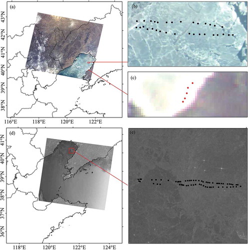
The ice thickness was collected via field measurements. The ice samples were cut out from the ice at different locations using an ice breaker on board when the satellite passed over on 14 February 2011. Then, we measured the thickness of each ice sample using a ruler. For the rough ice samples, we measured each several times at different locations, and the mean of the measured thicknesses was considered as the thickness of the sample. The measurement accuracy is 0.1 cm, and the position of the sampling point was recorded using a global positioning system (GPS) Pocket Terminal. We collected 37 samples (32 on the sea and 5 near the coast) of level sea ice and 65 samples of rough sea ice. The locations of the samples are shown in Figure 2(b), (c) and (e). Additional data were acquired by field measurements for the sea ice thickness, and reflectance spectrum data in 350–2500 nm band were also collected during the same period using an analytical spectral devices (ASDs) Field Spec 3 spectroradiometer.

2.2. Atmospheric correction of the HJ-1B CCD images

At the top of atmosphere (TOA), for ideal land surface and atmospheric conditions, the apparent reflectance of the VIS/NIR bands that were observed by the HJ-1B CCD sensor (Vermote et al. 1997) was calculated as follows:

(1)

where is the TOA reflectance; is the wavelength; is the reflectance of the surface; is the upward reflectance of the atmosphere, including Rayleigh scattering and aerosol scattering; is the total upward transmittance of the atmosphere; is the total downward transmittance of the atmosphere; and is the downward hemispherical reflectance of the atmosphere. Due to the lack of atmospheric measurement data synchronized with the HJ-1B CCD images, we employed a standard atmospheric model and an aerosol model for the atmospheric correction (winter in the middle latitude, sea type). We used the measured visibility data (33 km) from the weather station; then, we entered the atmospheric parameters, satellite observation parameters and the sensor spectral response function into the Second Simulation of the Satellite Signal in the Solar Spectrum (6S) software to calculate , , and , which are in Equation (1) (Vermote et al. 1997). In order to calculate , it was necessary to calibrate the HJ-1B CCD images. The calibration method was as follows:

(2)

where is the radiance, is the digital number (DN) value of the pixel, is the band number, and and are the calibration coefficients, which were provided and validated by the China Resources Satellite Application Center (China Center for Resources Satellite Data and Application 2010). After the calculation of TOA reflectance, the formula for retrieving surface reflectance is calculated as follows:

(3)

Although the reflection of a surface is in fact anisotropic (Xu et al. 2010), in this article, the surface reflectance was calculated under the assumption that the reflection of the surface is isotropic since there are not enough multiangle remote sensing images to calculate the hemisphere directional reflectance, which takes the surface bidirectional reflectance distribution function (BRDF) into consideration.

2.3. ENVISAT ASAR image radiometric calibration and noise removal

ENVISAT ASAR images can be calibrated using the Next ESA SAR Toolbox (NEST) software package, which was developed by Array Systems Computing Inc. (Toronto, ON, Canada) for ESA (Rosich and Meadows 2004):

(4)

where is the backscattering coefficient, is the DN value of the image pixel, is the incident angle, and is the absolute calibration factor. There was speckle noise on the ENVISAT ASAR images due to interference effects. We filtered the ENVISAT ASAR images using the enhanced Lee filtering method to remove the noise (Shi and Fung 1994), and the filter window was 5 × 5.

2.4. Registration and resampling of the HJ-1 CCD and ENVISAT ASAR images

To register the ENVISAT ASAR image to the HJ-1 CCD image, 100 corresponding points, well distributed on the images, were selected manually. The geometric correction method for the ENVISAT ASAR image was the polynomial method, and the root mean square error (RMSE) was approximately 24.3 m within one pixel size. The resampling method of the ENVISAT ASAR image was the cubic convolution sampling method, and the resolution of resampled image was 30 m. The common portion of the two images was used for the study in this article.

2.5. Determination of the extent and division of level and rough sea ice

Considerable amounts of ice and snow cover the land around the Bohai Sea, and their reflection and scattering properties are very similar to those of sea ice. Therefore, it is difficult to differentiate the ice and snow on the land from sea ice. To solve this problem, the portion of the ENVISAT ASAR and HJ-1 CCD images defined as land was subtracted from each mosaic image using a mask of the Bohai Sea.

The masked HJ-1 CCD images were segmented, and an image containing numerous patches with pure reflectance spectra was obtained. The mean reflectance spectrum of each patch was calculated. The extent of the sea ice and sea water was determined from the image containing the patches using a support vector machine classification method (Vapnik 2000), which was based on a training sample set corresponding to the first and last 5% of the histogram of the mean reflectance spectra of all patches.

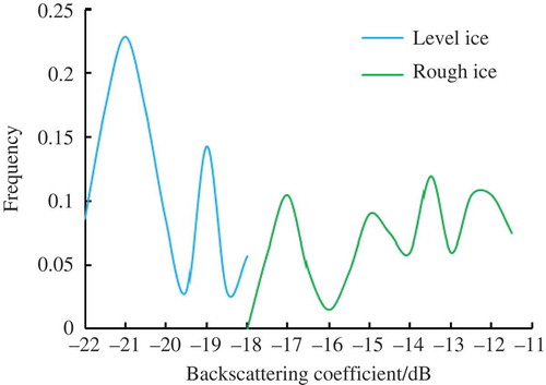
Several profile graphs of new ice and land-fast ice formed in static sea water and rough ice formed in flowing sea water were surveyed. The surveys showed that the root mean squared heights (RMSHs) of all level ice samples were less than 1 cm (Figure 3). However, the rough ice in the Bohai Sea always formed from crushed level ice, and the RMSHs were greater than 1 cm (Figure 3). Therefore, level ice was defined as the ice with an RMSH less than 1 cm, and the ice with an RMSH greater than 1 cm was regarded as rough ice. The extent of level and rough ice was determined from the ENVISAT ASAR image using a threshold of . The threshold value was determined by the cut-off value (see Figure 4) of the backscattering coefficients belonging to the level ice sample locations and the backscattering coefficients belonging to the rough ice sample locations (see Figure 2).

Figure 3. Profile graphs of the level ice and rough ice based on field observations. (a) Profile graph of level ice; (b) profile graph of rough ice; z is the height relative to the average height, and x is the horizontal coordinate.

Figure 4. Histogram of level/rough ice backscattering coefficient.

3. Results and analysis

3.1. Extent of sea ice, level ice and rough ice

From Figure 5, it can be observed that the sea ice extent extracted from the HJ-1 CCD image was more precise. The narrow leads and texture were more clearly evident in the ice extent map extracted from HJ-1 CCD and ASAR images (Figure 5(a)) than from the MODIS image (Figure 5(b)), especially for the circled parts in Figure 5(a) and (b). Compared with the ENVISAT ASAR images, the HJ-1 CCD images were more suitable for the extraction of the sea ice extent, which can be attributed to a more clear distinction of the back scattering coefficients of sea water and smaller areas of rough ice. However, the ENVISAT ASAR images were more suitable for distinguishing between level ice and rough ice compared with the HJ-1 CCD images because of a clearer distinction of the reflectance spectrum of rough ice and thicker ice. It is worth mentioning that there was striping noise in Figure 5 that originated from the original image, which likely resulted from the systematic deviation during the mosaic of subswaths. In this article, the aim was to discuss the methodology used to estimate sea ice thickness, and the error is limited. So we did not consider it a significant source of error.

Figure 5. The extents of sea ice, level ice and rough ice. (a) Extracted from HJ-1 CCD and ASAR images; (b) extracted from MODIS image acquired on 14 February 2011 02:30 am UTC.

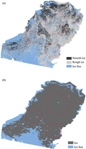
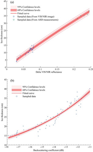
Figure 6. Relationship between the thickness of the level sea ice and the reflectance and the relationship between the thickness of rough sea ice and the backscattering coefficient. (a) Relationship between the thickness of the level sea ice and reflectance; (b) relationship between the thickness of rough sea ice and the backscattering coefficient. The blue circles represent the field measurements; the pink line is the fitted curve; the deep pink region corresponds to the 95% confidence interval, and the light pink region corresponds to the 68% confidence interval.

3.2. Relationship between the thickness and reflectance of level sea ice

For level ice, the reflectance increases with the thickness of sea ice when the viewing zenith is 0° or nearly 0°. This is because the reflected energy originates primarily from the volume scattering of sea ice, and the contribution from the sea ice surface is very small. Figure 6(a) shows the relationship between level sea ice thickness and reflectance. The VIS/NIR reflectance in Figure 6(a) was calculated from the atmospheric correction images of bands 1 through 4 using a weighted average method. This reflectance can express the overall characteristics of sea ice reflection in the VIS/NIR band. The formula for the calculation is as follows:

(5)

where is the reflectance of band , and is the weight of band , determined by normalizing the variance of reflectance of each band of the HJ-1 CCD image. The formula for the calculation is as follows:

(6)

where is the variance of band ; is the reflectance of pixel in the image of band .

The reflectance of sea water may be different in different zones of the Bohai Sea due to sediment brought in by the rivers that enter the Bohai Sea. Therefore, there may also be differences in the reflectance of the sea ice with the same thickness floating on such sea water. To eliminate errors of this type, the delta VIS/NIR reflectance was calculated by subtracting the VIS/NIR reflectance of the nearest sea water pixels from the target sea ice pixels. The formula for the calculation is as follows:

7

where is the delta VIS/NIR reflectance, and is the VIS/NIR reflectance of the nearest sea water pixels.

All 37 field observations of the thickness of level ice are shown in Figure 6(a). Among these, 32 of the data points were sampled during the ENVISAT satellite transition, and the corresponding VIS/NIR reflectance was selected from the VIS/NIR reflectance image calculated using Equation (4). The remaining five data points represent the level sea ice thickness and the corresponding VIS/NIR reflectance measured on the ground using an ASD Field Spec 3 spectroradiometer at the same time. The curve in Figure 6a was fitted to the relationship between the thickness of level sea ice and the delta VIS/NIR reflectance on the basis of the field-measured data (blue circles in Figure 6(a)), and the expression for the fitted curve is:

(8)

where is a coefficient with a value of 319.5 determined using a robust regression. Table 2 provides the goodness of the fit. The R² was 0.99, and the RMSE was 1.0 cm. Therefore, it is clear that the relationship between the thickness of the level sea ice and the delta VIS/NIR reflectance is logarithmic, which is in agreement with the results reported by Xie et al. (2006). For the same thickness, the reflectance in Equation (8) may vary with the solar zenith, because different solar zeniths correspond to different scattering angles. Therefore, the reflectance inputted into Equation (8) should be rectified according to the model of the reflectance by varying with the solar zenith, which can be summarized from field measurements.

Table 2. Goodness of the fit.

	R^2	RMSE (cm)
Level sea ice	0.988	0.978
Rough sea ice	0.899	2.252

3.3. Relationship between the thickness of rough sea ice and the backscattering coefficient

The backscattering energy results mainly from sea ice surface scattering and volume scattering. When the sea ice is thin or the sea ice surface is smooth, penetration of microwave radiation is non-negligible (Zhang 2011), and there may be some scattering energy from the sea water. The surface scattering energy may be much larger than that of the volume scattering when the sea ice surface is rough. The regression curves for the rough ice thickness and backscattering coefficients are shown in Figure 6(b). A total of 65 sea ice samples were collected during the transit of ENVISAT. The fitted curve was also obtained through the robust regression, and the formula is:

9

where is the backscattering coefficient of rough sea ice in the Bohai Sea; c₁ and c₂ are coefficients with values of 203.8 and 0.1504, respectively. The goodness of fit is presented in Table 2. The R² was 0.90, and the RMSE was 2.3 cm. It is obvious that the relationship between the thickness and the backscattering coefficient of the rough sea ice was exponential. The results support the conclusions drawn by Nakamura et al. (2009) for the first-year ice in the Lützow-Holm Bay. Although Nakamura et al. (2009) argued that the ratio of the VV and HH backscattering coefficients was relevant to the salinity and thickness of the sea ice, we believed it was feasible to estimate the thickness of the sea ice in the Bohai Sea, which is only half the thickness of that in Lützow-Holm Bay, and the variation in the salinity relative to the ice thickness is relatively small.

3.4. Estimated sea ice thickness in the Bohai Sea

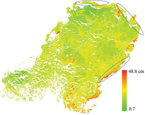
The sea ice thicknesses were calculated using Equations (7) and (8) in Figure 7. The sea ice thickness shown in Figure 7 is basically consistent with the general situation based on the expectations from previous studies (Yuan et al. 2012). The ice barrier line of the land-fast ice is very clear (see blue ellipses in Figure 7). The maximum sea ice thickness is approximately 48.8 cm, and the mean ice thickness is 18.6 cm.

Figure 7. The map of the sea ice thickness in the Bohai Sea.

4. Discussions and conclusions

4.1. Discussions

The reflection and scattering of sea ice in solar and microwave bands is a complex process, and currently, there is no analytic model that can depict this precisely. In this article, the empirical model used to estimate sea ice thickness in the Bohai Sea was proposed through satellite synchronous observation. The sources of errors in our experiment originate primarily come from: (1) the inversion of surface reflectance of the HJ-1 CCD image; (2) the image registration and resampling of the HJ-1 CCD and ENVISAT images; (3) the calibration of the ENVISAT image, for example, the striping noise in the image used in this article; (4) errors between the measured sea ice thickness, which are point data, and the sea ice thickness at the corresponding pixels, namely the errors associated with the point data and the area data. The proposed empirical models are shown to be feasible and practical according to the estimation of the sea ice in the Bohai Sea conducted in this article, though we have performed a single test; (5) the error caused by the disparate solar zeniths. The reflectance may vary with the solar zenith, because different solar zeniths result in different scattering angles. However, the reflectance can be rectified based on the model of the reflectance by varying with the solar zenith which may be summarized from the field measurements; (6) the variation of the backscattering coefficient with the varying incident angle for the same thickness. Similar to sea ice reflectance, the backscattering coefficient can also be rectified according to the related model; (7) the error caused by the variation of interior structure (the amount of brine pockets and bubbles) of sea ice, which can lead to a change in the scattering coefficient. This can be rectified by the modification of parameters in the model of sea ice thickness estimation; (8) influence of snow cover. Even with a very thin layer grammar corrections snow cover, the estimated level ice will be too large; (9) errors caused by unscreened clouds. Few unscreened cloud will make the estimated level ice thickness distorted.

In addition, there may be another limitation of the proposed empirical model in this article, since the methods were based on field measurements that were carried out in a small region and over a single day. The weather and sea ice conditions may be different for other images at other times. We believe that the reflectance discrepancy caused by weather conditions can be eliminated through the accurate atmospheric correction. For the sea ice condition at different times, the extinction (absorption and scattering) coefficient of level and rough sea ice is basically the same for the entire Bohai Sea, except for the melt season. Regardless, the model proposed in this article still needs to be verified against more images acquired at different times of the winter (especially in the melt season) and different viewing geometries to ensure that it is robust for future use.

In fact, it is an intractable task to retrieve precise ground surface parameters from remote sensing data, due to their incompleteness and the complexity of the earth system at present. To conduct an estimation of the sea ice thickness more authoritatively using remote sensing images of the Bohai Sea, the parameters for the sea ice reflection, emission and scattering processes must be determined more correctly in the future. To achieve this, we must combine multiple remote sensing images obtained simultaneously, including multiwavelength, multiangle and multiremote sensing mode images. For example, according to the multistage and multiobject decision strategy and prior knowledge, we could retrieve more sensible parameters (such as the surface roughness, bubble size and brine pocket ratio) relative to specific remote sensing images of sea ice and then estimate other parameters (for example, the sea ice thickness) (Li and Strahler 1996; Hu et al. 1997; Li et al. 2001). Increasing numbers of remote sensing images will be obtained by different satellite and remote sensors, and the development of remote sensing technology will continue. Multistage and multiobject decisions are a potentially useful strategy for precise estimates of the sea ice thickness precisely in the Bohai Sea.

4.2. Conclusions

The estimation of sea ice thickness in the Bohai Sea is a particularly important problem in the area of sea ice remote sensing. We conducted a preliminary experiment to estimate the thickness of the sea ice in the Bohai Sea by combining VIS/NIR (HJ-1 CCD) and SAR (ENVISAT) images using our proposed empirical models. Based on this experiment, we arrive at the following conclusions: (1) VIS/NIR remote sensing images are more suitable for determining the sea ice extent, and SAR images are more suitable for distinguishing between level and rough sea ice in the Bohai Sea; (2) in the Bohai Sea, the relationship between the level ice and VIS/NIR reflectance is logarithmic, and the relationship between backscattering and rough ice is exponential.

Disclosure statement

No potential conflict of interest was reported by the authors.

Acknowledgements

We are thankful to anonymous reviewers for their valuable comments and suggestions. We also thank LetPub (www.letpub.com) for its linguistic assistance during the preparation of this manuscript.

Additional information

Funding

This paper was supported by science and technology projects of the Chinese government: National High Technology Research and Development Program of China [No. 2011AA100505] and project supported by State Key Laboratory of Earth Surface Processes and Resource Ecology [2010-KF-08].

References

- Campbell, J. B., and R. H. Wynne. 2011. Introduction to Remote Sensing. 5th ed., 31–57. New York: Guilford Press.
- China Center for Resources Satellite Data and Application (CCRSDA). 2009. “An Introduction of HJ-1A, B Satellite.” http://www.cresda.com/n16/n1130/n1582/8384.html 2013.01 [In Chinese.]
- China Center for Resources Satellite Data and Application (CCRSDA). 2010. “On-Orbit Absolute Radiometric Calibration Coefficients of HJ-1A, B Satellite in 2010.” http://www.cresda.com/n16/n1115/n1522/n2103/index.html. 2013.01 [In Chinese.]
- Deng, S. Q. 1986. “Sea Ice Disaster in Bohai Sea and the General Situation of Its Prevention.” [In Chinese.] Journal of Catastrophology 1: 80.
- Ding, D. W. 1999. An Introduction to Engineering Sea Ice, 1–70. Beijing: China Ocean Press. [In Chinese.]
- European Space Agency (ESA). 2002. “ASAR.” https://earth.esa.int/web/guest/missions/esa-operational-eo-missions/envisat/instruments/asar
- Feng, S. Z., F. Q. Li, and S. J. Li. 1999. An Introduction of Maritime Science, 463. Beijing: Higher Education Press. [In Chinese.]
- Filippi, A. M., B. L. Bhaduri, T. Naughton, A. L. King, S. L. Scott, and I. Güneralp. 2012. “Hyperspectral Aquatic Radiative Transfer Modeling Using a High-Performance Cluster Computing-Based Approach.” GIScience & Remote Sensing 49 (2): 275–298. doi:10.2747/1548-1603.49.2.275.
- Finnish Meteorological Institute (FMI). 2014. “Ice Thickness Chart and Ice Forecast”. Accessed February 10. http://haavi.fimr.fi/polarview/index.php
- Grenfell, T. C. 1983. “A Theoretical Model of the Optical Properties of Sea Ice in the Visible and near Infrared.” Journal of Geophysical Research 88 (C14): 9723–9735. doi:10.1029/JC088iC14p09723.
- Grenfell, T. C., and D. K. Perovich. 1981. “Radiation Absorption Coefficients of Polycrystalline Ice from 400-1400 Nm.” Journal of Geophysical Research 86 (C8): 7447–7450. doi:10.1029/JC086iC08p07447.
- Gu, W., Y. Lin, Y. J. Xu, S. Yuan, J. Tao, L. Li, and C. Liu. 2012. “Sea Ice Desalination under the Force of Gravity in Low Temperature Environments.” Desalination 295: 11–15. doi:10.1016/j.desal.2012.03.017.
- Guo, F. L., R. Y. Zhao, and W. B. Wang. 2000. “Application of Passive Microwave Remote Sensing to Sea Ice Thickness Measurement.” [In Chinese.] Journal of Remote Sensing, 4 (2): 112–117.
- Guo, Q. Z., W. Gu, J. Li, Z. Liu, and Y. H. Chen. 2008. “Research on the Sea Ice Disaster Risk in Bohai Sea Based on the Remote Sensing.” [In Chinese.] Journal of Catastrophology 23 (2): 10–14.
- Hu, B. X., W. Lucht, X. W. Li, and A. H. Strahler. 1997. “Validation of Kernel-Driven Semiempirical Models for the Surface Bidirectional Reflectance Distribution Function of Land Surfaces.” Remote Sensing of Environment 62: 201–214. doi:10.1016/S0034-4257(97)00082-5.
- Karvonen, J., B. Cheng, and M. Similä. 2007. “Baltic Sea Ice Thickness Charts Based on Thermodynamic Ice Model and SAR Data.” In Geoscience and Remote Sensing Symposium, 2007 (IGARSS 2007), Barcelona, July 23–28, 4253–4256. Piscataway, NJ: Institute of Electrical and Electronics Engineers.
- Karvonen, J., B. Cheng, M. Similä, and M. Hallikainen. 2008. “Baltic Sea Ice Thickness Charts Band on Thermodynamic Snow/Ice Model, C-Band SAR Classification and Ice Motion Detection.” In Geoscience and Remote Sensing Symposium, 2008 (IGARSS 2008), IV, Boston, MA, July 7–11, 173–176. Piscataway, NJ: Institute of Electrical and Electronics Engineers.
- Li, X. W., and A. Strahler. 1996. “A Knowledge-Based Inversion of Physical BRDF Model and Three Examples.” In International Geoscience and Remote Sensing Symposium, IGARSS 96, Lincoln, NE, May 27–31, 2173–2176. Piscataway, NJ: Institute of Electrical and Electronics Engineers.
- Li, X. W., J. F. Wang, J. D. Wang, and Q. H. Liu. 2001. Multi Angle and Thermal Infrared Remote Sensing of the Earth, 71–150. Beijing: Science Press.
- Liu, C., W. Gu, J. Chao, L. Li, S. Yuan, and Y. Xu. 2013. “Spatio-Temporal Characteristics of the Sea-Ice Volume of the Bohai Sea, China, in Winter 2009/10.” Annals of Glaciology 54 (62): 97–104. doi:10.3189/2013AoG62A305.
- Luo, Y. W., Y. F. Zhang, C. R. Sun, H. D. Wu, X. H. Cai, Y. Liu, S. Bai, and Z. G. Jin. 2005. “Application of The/HY-10 Satellite to Sea Ice Monitoring and Forecasting.” [In Chinese.] ACTA Oceanologica Sinica 27 (1): 7–18.
- Nakamura, K., H. Wakabayashi, S. Uto, S. Ushio, and F. Nishio. 2009. “Observation of Sea-Ice Thickness Using ENVISAT Data From LÜtzow-Holm Bay, East Antarctica.” IEEE Geoscience and Remote Sensing Letters 6 (2): 277–281. doi:10.1109/LGRS.2008.2011061.
- Ning, L., F. Xie, W. Gu, Y. Xu, S. Huang, S. Yuan, W. Cui, and J. Levy. 2009. “Using Remote Sensing to Estimate Sea Ice Thickness in the Bohai Sea, China Based on Ice Type.” International Journal of Remote Sensing 30: 4539–4552. doi:10.1080/01431160802592542.
- Pereira, L. O., C. C. Freitas, and S. J. Siqueira St Anna. 2013. “Optical and Radar Data Integration for Land Use and Land Cover Mapping in the Brazilian Amazon.” GIScience & Remote Sensing 50 (3): 301–321.
- Rosich, B., and P. Meadows. 2004. “Absolute Calibration of ASAR Level 1 Products Generated with PF-ASAR.” ESA/ESRIN, ENVI-CLVL-EOPG-TN-03-0010, 10 (1): 5–6.
- Sheorana A., Haackb B. 2013. “Classification of California Agriculture Using Quad Polarization Radar Data and Landsat Thematic Mapper Data.” GIScience & Remote Sensing 50 (1): 50–63.
- Shi, Z., and K. B. Fung. 1994. “A Comparison of Digital Speckle Filters.” In International Geoscience and Remote Sensing Symposium, IGARSS 1994, Pasadena, CA, August, 8–12, 2129–2133. Piscataway, NJ: Institute of Electrical and Electronics Engineers.
- Similä, M., M. Mäkynen, B. Cheng, and J. Karvonen. 2010. “Sea Ice Thickness Chart Based on the SAR and MODIS Data.” 38th COSPAR Scientific Assembly, Bremen, July 15–18, 5.
- State Oceanic Administration People’s Republic of China (SOAPRC). 2012. Statistical Communique of Marine Economy of China in 2011. State Oceanic Administration People’s Republic of China. http://www.soa.gov.cn/ [In Chinese.]
- Stogryn, A., and G. J. Desargant. 1985. “The Dielectric Properties of Brine in Sea Ice at Microwave Frequencies.” IEEE Transactions on Antennas and Propagation 33 (5): 523–532. doi:10.1109/TAP.1985.1143610.
- Toyota, T., S. Ono, K. Cho, and K. I. Ohshima. 2011. “Retrieval of Sea-Ice Thickness Distribution in the Sea of Okhotsk from ALOS/PALSAR Backscatter Data.” Annals of Glaciology 52 (57): 177–184. doi:10.3189/172756411795931732.
- Tsang, L., J. A. Kong, and K. H. Ding. 2004. Scattering of Electromagnetic Waves, Theories and Applications. New York: John Wiley & Sons.
- Ulaby, F. T., R. K. Moore, and A. K. Fung. 1986. Microwave Remote Sensing: Active and Passive, Volume II: Radar Remote Sensing and Surface Scattering and Emission Theory, 1065–1156. Boston, MA: Artech House Publishers.
- Vapnik, V. 2000. The Nature of Statistical Learning Theory. New York: Springer.
- Vermote, E. F., D. Tanre, J. L. Deuze, M. Herman, and J.-J. Morcette. 1997. “Second Simulation of the Satellite Signal in the Solar Spectrum, 6S: An Overview.” IEEE Transactions on Geoscience and Remote Sensing 35 (3): 675–686. doi:10.1109/36.581987.
- Wu, K. Q., Y. Xu, and Y. M. Hao. 2005. “Application Sea Ice Remote Sensing of MODIS Data.” [In Chinese.] Maritime Forecasts (Supplement), 22 (Z1): 44–49.
- Wu, L. T., H. D. Wu, L. T. Sun, Y. F. Zhang, Y. Liu, and X. Q. Wei. 2006. “Retrieval of Sea Ice in the Bohai Sea from MODIS Data.” [In Chinese.] Periodical of Ocean University of China 36 (2): 173–179.
- Xie, F., W. Gu, S. Ha, W. Cui, W. Chen, C. Zhou, S. Huang, and Z. Liu. 2006. “An Experimental Study on the Spectral Characteristics of One Year-Old Sea Ice in the Bohai Sea, China.” International Journal of Remote Sensing 27 (14): 3057–3063. doi:10.1080/01431160600589153.
- Xie, F., W. Gu, Y. Yuan, and Y. H. Chen. 2003. “Estimation of Sea Ice Thickness for Sea Ice Resources in Liaodong Gulf Using Remote Sensing.” [In Chinese.] Resources Science 25 (3): 17–23.
- Xie, S. M., D. Z. Jiang, B. Zou, and Z. H. Xue. 2002. “Role of Sea Ice in Air-Sea Exchange and Its Relation to Sea Fog.” [In Chinese.] Polar Research 14 (1): 44–56.
- Xu, Z. T., Y. Z. Yang, G. F. Wang, W. X. Cao, and X. P. Kong. 2010. “Reflectance of Sea Ice in Liaodong Bay.” [In Chinese.] Spectroscopy and Spectral Analysis 30 (7): 1902–1907.
- Yang, G. J. 2000. Sea Ice Engineering. 1–90, 455–480. Beijing: Petroleum Industry Press. [In Chinese.]
- Yuan, S., W. Gu, Y. J. Xu, P. Wang, S. Huang, Z. Le, and J. Cong. 2012. “The Estimate of Sea Ice Resources Quantity in the Bohai Sea Based on NOAA/AVHRR Data.” ACTA Oceanologica Sinica 31 (1): 33–40. doi:10.1007/s13131-012-0173-4.
- Zhang, X. 2011. Research on Sea Ice Thickness Detection by Polarimetric SAR in Bohai Sea. The Graduate School of Ocean University of China. [In Chinese.]