Image simulation from multitemporal landsat images

Abstract

Multitemporal datasets can provide information on the different acquisition patterns of pixel values. The resultant generation of simulated images based on these patterns becomes practical and easy. In this paper, we propose a simple model for creating a simulated image based on a set of multitemporal satellite images and meteorological data utilizing a temporal correlation of multitemporal images. The satellite images and meteorological data used for the model can be easily accessed through open data sources. A dataset of 55 Landsat images was used to determine the relationship between the spectral radiance of the pixels and solar radiation, air temperature, humidity, rainfall, and visibility based on a multilinear regression analysis. This multilinear regression equation was then used to generate the simulated images obtained on the target dates. The results indicate that more than 91% of the pixels of the simulated images have correlation coefficients greater than 0.98 in all experimental cases. The correlation coefficients increased significantly when the normalized difference vegetation index (NDVI) and a reference image were applied to the man-made areas. The quality of the simulated images generated by this model primarily depends on changes in land cover. However, this effect can be reduced using NDVI interpolated from images obtained during the same season, or by employing a reference image acquired close to the date on which the simulated image is generated.

Keywords:

• image simulation
• Landsat image
• multitemporal image
• solar radiation
• meteorological parameters

Introduction

Simulation and modeling can be valuable tools for generating simulated datasets and evaluating data processing algorithms (Guanter, Segl, and Kaufmann 2009). These tools are cost-effective approaches to predicting the performance characteristics of future sensors before the physical components are designed (Blonski et al. 1997). For example, image simulation has been applied to simulate realistic radar reflectivity acquisitions in support to the mission design of Sentinel-1, which is a new generation of imaging synthetic aperture radars (SARs) of the European Union (EU) and the European Space Agency (ESA) (Sabel et al. 2012). In addition, the results of the image simulation can be used to determine optimal flight paths (Stark 1993; Kim et al. 2013).

For a more effective use of satellite measurements, it is necessary to understand what type of performance can be expected from the sensors used. Therefore, the generation of diverse images simulated under the same performance conditions is needed (Blaschke 2010). Schott et al. (1999) developed a model called digital imaging and remote sensing image generation (DIRSIG) for simulating multi- and hyperspectral images using a ray-tracing technique. To support the validation of the advanced spaceborne thermal emission and reflection radiometer (ASTER) and moderate resolution imaging spectroradiometer (MODIS) geographical retrieval algorithms, and to provide additional radiometric calibrations, Hook et al. (2001) developed the MODIS/ASTER airborne simulator (MASTER). This model propagates the surface reflectance, which is measured using a spectrometer, to the at-sensor radiance using radiative transfer models. Guanter, Segl, and Kaufmann (2009) developed an optical hyper- and multispectral scene simulator within the environmental mapping and analysis program (EnMAP) mission framework. This method generates simulated images using several sequential processing modules related to natural environments, acquisition and illumination geometries, cloud cover conditions, and instrument configurations. Another model was proposed by Zhao et al. (2013) to simulate hyperspectral images over rugged scenes with a consideration of the adjacency effects. This simulation is based on physical principles involving atmospheric, topographic, and adjacency effects, as well as sensor response and noise. To calculate the atmospheric parameters used to simulate at-sensor radiance, the above methods typically use a radiative transfer code, such as moderate resolution atmospheric transmission (MODTRAN) (Berk et al. 1999; Hook et al. 2001; Guanter, Segl, and Kaufmann 2009; Zhao et al. 2013), low altitude atmospheric transmission (LOWTRAN) (Carl, Joseph, and John 1993), or second simulation of a satellite signal in the solar spectrum (6S) (Vermote et al. 1997; Gascon, Gastellu-Etchegorry, and Lefevre 2001). However, it is not easy to efficiently employ these tools; moreover, they are not readily available to the general public (Schläpfer and Nieke 2005).

In recent years, numerous multispectral and hyperspectral remote sensing satellites with diverse resolutions have been built, launched, and operated (S. Chen et al. 2013). As a result, many satellite images have been collected and archived (Lin et al. 2013). However, conventional studies have used only the latest high-resolution images or leveraged the fusion between limited sensors. Furthermore, few time-series or multi-resolution image-based studies have been conducted. It is therefore necessary to conduct scientific research that takes advantage of datasets containing a substantial amount of image data (Lin et al. 2013).

One disadvantage of a passive remote sensing sensor is its high sensitivity to weather conditions when acquiring images. Consequently, images are often affected by cloud cover; this compromises the usability of optical remote sensing and further complicates the image processing (Ju and Roy 2008). However, the pattern of pixel values based on the season and weather changes determined from substantial remote sensing data within a region can aid the reconstruction of data that is missing on account of the presence of clouds. In addition, the Sun is the energy source used in passive remote sensing. As a result, in wavelengths ranging from 0.4 to 2.5 µm, the total radiance that reaches a sensor observing a rugged scene is a complex signal with atmospheric and topographic properties (Zhao et al. 2013). For remote sensing within the visible and near-infrared (VNIR) region, the reflected radiance that is recorded by a sensor is affected by numerous parameters. These parameters include the solar and view geometry, spectral reflectance of the ground material under observation, surface orientation, and bidirectional reflectance properties, as well as the atmospheric absorption and scattering from gases (water vapor, ozone, carbon monoxide, carbon dioxide, etc.), atmospheric particles, and the temperature (Salisbury 1998). Nevertheless, determining the set of parameters for predicting the at-sensor radiance is not a trivial task (Cao et al. 1999).

The spectral radiance measured by a sensor is affected by many factors. Therefore, the correlation between the spectral radiance and the impact factors is very complex. This can be expressed as a linear or nonlinear function. In this study, a linear model is preferred because of its simplicity. To simplify the simulation process, we developed a basic model for generating simulated images based on a readily accessible dataset by leveraging the temporal relationships among multitemporal images. The dataset includes multitemporal satellite images, a digital elevation model (DEM), and meteorological conditions obtained from open data sources. Realistic radiance images are generated through several processing steps in which atmospheric, terrain, and shadow effects are considered. First, solar radiation on the dates of acquisition is modeled based on ASTER Global DEM (GDEM). Then, multilinear regression is conducted to find the temporal correlation between the pixel values and the solar radiation, air temperature, humidity, rainfall, and visibility. Finally, based on this relationship, new pixel values on the target date are computed. The simulated image is then compared with the actual image to assess the quality.

Study sites and materials

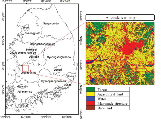
The study site was a 24 km × 24 km area partly covering Iksan and Gimje in the Republic of Korea, which is approximately 180 km south of Seoul (see Figure 1). The study area was limited to increase the number of images used for the multilinear regression. Agricultural fields occupy most of the study area; however, it additionally includes a few high-rise residential areas and some public and commercial buildings. The area is partly covered by forest areas and has substantial tree cover. Korea has four very distinct seasons: spring, which is from March to the end of May; summer, which is from June through August; autumn, which is from September through November; and winter, which is from December to the end of February (Korean Meteorological Administration 2015). Spring begins with the sprouting of various species of trees and the first crops of strawberries. Summer is relatively hot and humid and may feature clouds and frequent rainfall for 1–3 weeks. In autumn, as the season progresses, the leaves change colors and harvesting begins. Winter is generally cold and dry, and snow typically occurs in December and January. To avoid an image with snow cover, images obtained in December, January, and February were excluded. A dataset of 55 satellite images acquired from March to November of 1991–2014 was used. Forty-four Landsat 5 thematic mapper (TM) images, four Landsat 7 enhanced thematic mapper plus (ETM+) images, seven Landsat 8 images, and ASTER GDEM were freely obtained from the US Geological Survey (USGS) (http://earthexplorer.usgs.gov/). Along with this dataset, meteorological data (i.e., air temperature, humidity, rainfall, and visibility) at two ground stations (indicated by red triangles in Figure 1) near the study area were obtained from the Korean Meteorological Administration (KMA) (http://www.kma.go.kr).

Figure 1. Study area and a land cover map. For full color versions of the figures in this paper, please see the online version.

Methodology

Preprocessing

After downloading the satellite images, radiometric calibration was conducted to convert the digital numbers (DNs) into spectral radiance. The wavelengths of band 1 of the Landsat 8 images differ from those of the Landsat 5TM and ETM+ images; hence, band 1 of the Landsat 8 images was excluded. A subset containing 800 × 800 pixel images covering the study site was then selected. To increase the number of satellite images, some Landsat images with a small amount of cloud cover were also included (maximum cloud coverage of selected images is 10%). Therefore, it was necessary to mask cloud pixels before the analysis. With these images, a cloud mask was generated based on a cloud-screening algorithm described by Ouaidrari and Vermote (1999) (see that work for more details on the cloud-screening algorithm). Based on the cloud mask, cloudy pixels were excluded and only clear pixels were used in further analyses. In addition, the dataset contained images acquired at different times; therefore, a shadow cast by high features, such as high buildings and mountains, was also different. This could have led to the decreased quality of the simulated image. To reduce this effect, a shadow mask for each image was additionally created based on ASTER GDEM. This was carried out by using MATLAB based on algorithm described in Gill (2012). This method applies ray-tracing technique to project shadows: a point is in a shadow if the straight line from that point to the light source is blocked (Gill 2012).

Solar radiation modeling

The solar radiation incident on the earth’s surface is both shortwave and long wave radiation. The shortwave radiation reaching the surface of the earth consists of three components: direct, diffuse, and reflected radiation (Kumar, Skidmore, and Knowles 1997). Several approaches have been proposed to calculate the amount of solar radiation reaching the earth’s surface. In this study, the method described by Kumar, Skidmore, and Knowles (1997) for solar radiation estimation was used. This method is based on the model described in Gates (1980), and the three components of solar radiation can be computed by Equations (1)–(3) (Gates 1980). For further details on estimating the amount of solar radiation please refer to Kumar, Skidmore, and Knowles (1997). This algorithm can be utilized to estimate the amount of solar radiation over large areas of forest, ecological, and agricultural areas, and to study the variations of radiation under different aspects and slopes (i.e., considering the solar elevation angle and solar azimuth angle) (Kumar, Skidmore, and Knowles 1997). As a result, it has been used in researches of diverse fields (Kumar and Skidmore 2000; Guisan et al. 2007; X. Chen et al. 2013).

(1) $I_{\mathrm{d}\mathrm{i}\mathrm{r}}=I_0{\tau }_{b}cosi$(1)

(2) $I_{\mathrm{d}\mathrm{i}\mathrm{f}\mathrm{f}}=I_0(0.271-0.294{\tau }_{\mathrm{b}}){cos}^2\frac{\beta }{2}sin\alpha$(2)

(3) $I_{\mathrm{r}}=r{I}_0\left(0.271+0.706{\tau }_{\mathrm{b}}\right){sin}^2\frac{\beta }{2}sin\alpha$(3)

where $I_{\mathrm{d}\mathrm{i}\mathrm{r}}$ is direct solar radiation; $I_{\mathrm{d}\mathrm{i}\mathrm{f}\mathrm{f}}$, diffuse solar radiation; $I_{\mathrm{r}}$, reflected solar radiation; $I_0,$ extraterrestrial radiation; ${\tau }_{\mathrm{b}},$ atmospheric transmittance for beam radiation; r, ground reflectance coefficient; i, the angle between the normal to the surface and the direction to the sun; $\beta ,$ the slope of the surface, and $\alpha$ is solar elevation angle.

Spectral similarity measurement

As previously mentioned, the images used in this study were obtained from 1991 to 2014; during that period, many land cover changes may have taken place, potentially resulting in an incorrect prediction of the pixel values in the simulated images. To minimize this effect, a reference image, which was acquired by the same sensor near the date on which the simulated image was to be generated, was used. While selecting reference image one should take into account the change rate of the simulation area. In this study, two reference images were selected for two different simulation dates: one was acquired in the similar season of the simulation and the other was acquired in the different season (years of acquisition of reference images are different from years of the simulations). A spectral correlation mapper (SCM) was used to assess the change in input pixels compared with the reference pixels. A SCM threshold was applied to exclude pixels that were considered to be changed pixels. In this study, empirical analysis showed that pixels with an SCM of less than 0.95 can represent different land cover classes. For example, a pixel belonging to a bare land class may belong to a human-made-structure class in the reference image. Therefore, the SCM threshold was initially set to 0.95. If the number of pixels (each pixel belonging to each image) whose SCM exceeded this threshold was less than 25, then the threshold was reduced until the number of pixels was greater than 25. This pixel threshold number was additionally determined after some iterative attempts. It was used to ensure that the multilinear regression can properly operate and can vary depending on the total number of input images. The pixels whose SCM was greater than the threshold (unchanged pixels) were used in the generation of the simulated image.

The SCM method employs Pearson’s correlation coefficient (R) to detect changes; it can be computed using Equation (4). SCM is advantageous on account of its capacity to detect false positives. SCM values range from −1 to +1. Large values indicate that two spectra are similar. If there is no difference between the two spectra, the SCM value should be 1 (Carvalho Júnior et al. 2011).

(4) $\mathrm{S}\mathrm{C}\mathrm{M}=\frac{\sum _{i=1}^{\mathrm{n}\mathrm{b}}\left(T{1}_i-\overline{T1}\right)\left(T{2}_i-\overline{T2}\right)}{\sqrt{\sum _{i=1}^{\mathrm{n}\mathrm{b}}{\left(T{1}_i-\overline{T1}\right)}^2\sum _{i=1}^{\mathrm{n}\mathrm{b}}{\left(T{2}_i-\overline{T2}\right)}^2}}$(4)

where T1 and T2 are the spectra of a certain pixel in each band in the first and the second images, respectively; $\overline{T1}$ and $\overline{T2}$ are the mean values of T1 and T2 of each pixel; nb is the number of bands in an image; and each pixel has a SCM value.

At-sensor radiance simulation

A simplified version of the governing equation for at-sensor radiance can be expressed as the following (Photon Research Associates (PRA) 1998):

(5) $L_{\mathrm{s}\mathrm{e}\mathrm{n}\mathrm{s}\mathrm{o}\mathrm{r}}=L_{\mathrm{s}\mathrm{o}\mathrm{l}\mathrm{a}\mathrm{r}}\times {\rho }_{\mathrm{B}\mathrm{R}\mathrm{D}\mathrm{F}}\times cos\left(z\right)+L_{\mathrm{s}\mathrm{k}\mathrm{y}}\times {\rho }_{\mathrm{d}\mathrm{i}\mathrm{f}\mathrm{f}\mathrm{u}\mathrm{s}\mathrm{e}}+L_{\mathrm{b}\mathrm{b}}\left(T\right)\times \epsilon \times {\tau }_{\mathrm{p}\mathrm{a}\mathrm{t}\mathrm{h}}+L_{\mathrm{p}\mathrm{a}\mathrm{t}\mathrm{h}}$(5)

where L_sensor denotes the at-sensor radiance, L_solar is the direct solar radiance, ρ_BRDF represents the target bidirectional reflectance, and cos(z) is the cosine of the solar zenith angle. In addition, L_sky denotes diffuse sky shine, ρ_diffuse represents diffuse reflectance, L_bb is blackbody radiance, and T is the target temperature, while ε denotes target emissivity, τ_path represents path transmittance, and L_path is path radiance.

As shown in Equation (5), the spectral radiance measured by a sensor is affected by many components. Therefore, the correlation between the at-sensor radiance and the impact factors is very complex. Among the impact factors, path radiance can be derived from optical thickness using an empirical relationship (Kaufman 1993). Meanwhile, the aerosol optical thickness can be estimated from relative humidity and ground observation of visibility (Gueymard 1995). Moreover, humidity and precipitation are also dominant factors in estimating water vapor absorption in the spectral radiance model (Gueymard 1995). Air temperature is an important parameter for estimating land surface temperature (Qin, Karnieli, and Berliner 2001). These parameters are additionally used in LOWTRAN and MODTRAN families. Furthermore, environmental and atmospheric conditions can impact bidirectional reflection distribution function (BRDF) patterns (Schill et al. 2004). To simplify the simulation process, seven important factors that have potential effects on the spectral radiance observed by a sensor were selected for the multilinear regression analysis. These factors include the air temperature, humidity, visibility, and rainfall, as well as the direct solar, diffuse solar, and reflected radiation. The positional data of the sun were not considered as predictors because they were used to estimate the amount of solar radiation.

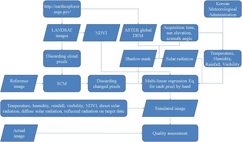
In this study, a simple model was developed for obtaining realistic spectral radiance images based on the temporal correlation of the multitemporal datasets. Most of the various processing stages applied in this model were performed using MATLAB; an overall summary is shown in Figure 2. First, preprocessing steps were conducted to prepare the data for the simulation procedure. Landsat images and ASTER GDEM were downloaded from the USGS EarthExplorer site (http://earthexplorer.usgs.gov/). The meteorological parameters, including the air temperature, humidity, rainfall, and visibility, were averaged from the values measured at the two ground stations. In this case, the rainfall was the total precipitation over 5 days before the image acquisition dates. The amount of solar radiation on the acquisition dates was estimated based on ASTER GDEM. A cloud mask was used to exclude cloud pixels, and the normalized difference vegetation index (NDVI) and a reference image was used to reduce the effect of changes in land cover. Multilinear regression available in MATLAB, which is an extension of the simple linear regression where multiple independent variables exist (Nathans, Oswald, and Kim 2012), was then conducted on each pixel, band by band, to determine the temporal relationship between the pixel values and the solar radiation, air temperature, humidity, rainfall, and visibility (and NDVI, if applied). This was conducted by considering the shading from the surrounding terrain. The multilinear regression equation of each pixel in each band was then used to estimate the pixel values on the target date. Finally, the simulated image was compared with the actual image to assess the quality.

Figure 2. Flowchart of the image simulation model.

In this study, we let $Y_b^k$ (k ∈ T = {T₁, T₂, …, T_M} and b ∈ B = {1, 2, …, N}) be the spectral radiance of N-channel images acquired and registered over the same geographical area at M different dates. Let $X_m^k$ be a set of predictors, including the humidity, air temperature, visibility, rainfall, direct solar radiation, diffuse solar radiation, and reflected radiation (k ∈ T, m = {1, 2, …, 7}). Here, the air temperature, humidity, rainfall, and visibility are single values; direct solar radiation, diffuse solar radiation, and reflected radiation are spatially distributed parameters. The complex relationship between the pixel values of Y, band by band, and predictor X are obtained through multilinear regression analysis. The multilinear regression equation used to estimate the pixel values of a simulated image can be expressed as Equation (6).

(6) $Y_{\left(i,j,b\right)}^t=a_{1\left(i,j,b\right)}{x}_1^t+a_{2\left(i,j,b\right)}{x}_2^t+a_{3\left(i,j,b\right)}{x}_3^t+a_{4\left(i,j,b\right)}{x}_4^t+a_{5\left(i,j,b\right)}{x}_{5\left(i,j\right)}^t+a_{6\left(i,j,b\right)}{x}_{6\left(i,j\right)}^t+a_{7\left(i,j,b\right)}{x}_{7\left(i,j\right)}^t+a_{8\left(i,j,b\right)}$(6)

where t is the target date, t∉T; i, j, and b are the row, column, and band number, respectively; and a₁ through a₈ are the regression coefficients. In addition, $x_1^t$ through $x_7^t$ are the air temperature, humidity, visibility, rainfall, direct solar radiation, diffuse solar radiation, and reflected radiation, respectively, on the target date, and Y is the spectral radiance value.

To reduce the land cover change effect on the simulation, NDVI, which is defined in Equation (7) (Rouse et al. 1974), was used as a predictor. In this case, Equation (8) was used to estimate the pixel value of the simulated image.

(7) $\mathrm{N}\mathrm{D}\mathrm{V}\mathrm{I}=\hspace{0.17em}\frac{R_{\mathrm{N}\mathrm{I}\mathrm{R}}-R_{\mathrm{R}\mathrm{e}\mathrm{d}}}{R_{\mathrm{N}\mathrm{I}\mathrm{R}}+R_{\mathrm{R}\mathrm{e}\mathrm{d}}}$(7)

(8) $Y_{\left(i,j,b\right)}^t=a_{1\left(i,j,b\right)}{x}_1^t+a_{2\left(i,j,b\right)}{x}_2^t+a_{3\left(i,j,b\right)}{x}_3^t+a_{4\left(i,j,b\right)}{x}_4^t+a_{5\left(i,j,b\right)}{x}_{5\left(i,j\right)}^t+a_{6\left(i,j,b\right)}{x}_{6\left(i,j\right)}^t+a_{7\left(i,j,b\right)}{x}_{7\left(i,j\right)}^t+a_{8\left(i,j,b\right)}{x}_{8\left(i,j\right)}^t+a_{9\left(i,j,b\right)}$(8)

where $x_8^t$ is NDVI on the target date.

Quality assessment

To evaluate the quality of the simulated images, several comparison approaches were conducted. For spectral features, SCM, which is described in the Spectral Similarity Measurement section, was used to compare the similarities between simulated and actual images. To assess the quantification of simulation errors, the relative root mean square error (RRMSE), which is a common measure that incorporates both random and systematic errors (Zhao et al. 2013), was calculated using Equation (9).

(9) $\mathrm{R}\mathrm{R}\mathrm{M}\mathrm{S}\mathrm{E}=\sqrt{\sum _{i=1}^C\sum _{j=1}^S\frac{{\left(\frac{L^{\mathrm{a}\mathrm{c}\mathrm{t}}\left(i,j\right)-L^{\mathrm{s}\mathrm{i}\mathrm{m}}\left(i,j\right)}{L^{\mathrm{a}\mathrm{c}\mathrm{t}}\left(i,j\right)}\right)}^2}{S\times C}}$(9)

where $L^{\mathrm{a}\mathrm{c}\mathrm{t}}\left(i,j\right)$ is the actual radiance at point (i,j), $L^{\mathrm{s}\mathrm{i}\mathrm{m}}\left(i,j\right)$ is the simulated radiance at point (i,j), and C and S are the respective numbers of rows and columns of the image.

Experiment

To study the validity of the simulation model, the model proposed in the Methodology section was used on three cases, with and without the aid of NDVI and the reference image, to generate the simulated images acquired on 22 September 2006, when crop lands were soon to be harvested, and on 11 March 2014, when crop lands were being planted. In the first case, multilinear regression was conducted to find the relationship among the pixel values and weather conditions (i.e., the air temperature, humidity, rainfall, and visibility), solar radiation (i.e., direct solar radiation, diffuse solar radiation, and reflected radiation) without the aid of NDVI and the reference image. Then, pixel values on simulation dates were computed using Equation (6).

In the second case, NDVI was used as a predictor to reduce the effect of land cover change. NDVI on the target date could be interpolated based on the NDVIs on the dates near the target date. In this study, NDVI on 22 September 2006 was linearly interpolated from the NDVIs on 31 August 2004 and 24 October 2006. Meanwhile, NDVI on 31 January 2014 was used as NDVI on 11 March 2014 because there was an insufficient number of appropriate images in the same season for the interpolation of NDVI on this date. In this case, Equation (8) was used to compute the pixel values of simulated images.

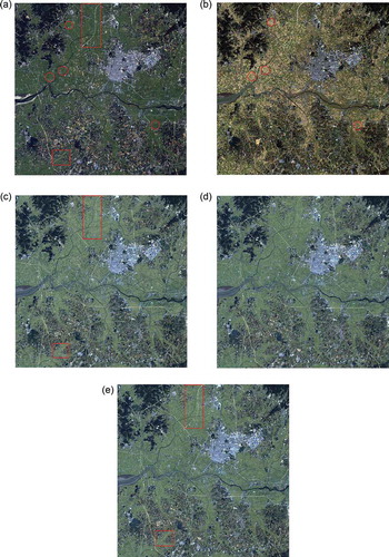
In the third case, in addition to using NDVI to reduce the effect of changes in land cover, an actual image was used as a reference. A Landsat 5 TM image obtained on 12 October 2005 was used for the simulation conducted on 22 September 2006; a Landsat 8 image acquired on 27 October 2013 was selected for the simulation on 11 March 2014. To detect changed pixels, SCM was used to measure the similarity between the input and reference pixels. The method for determining the SCM threshold is described in the Spectral Similarity Measurement section. Pixels below this threshold were excluded. However, this discarding was applied only to the human-made-structure pixels, which was extracted from classification result of reference image. In this study, maximum likelihood classification (MLC) available in ENVI software was used to classify reference image. Other features, such as grasslands and agricultural areas, can substantially change over a short time. For instance, in the study area, crop land is harvested in October; consequently, most of the same crop lands in the image obtained on 22 September 2006 were bare lands in the image acquired on 12 October 2005. Examples of this discrepancy are indicated by red circles in Figure 3(a) and (b). Therefore, the discarding of changed pixels was not applied to these features.

Figure 3. Images in their natural colors for the 22 September 2006 target date: (a) actual image obtained on the target date; (b) reference image acquired on 12 October 2005; (c) simulated image without NDVI and the reference image; (d) simulated image using NDVI; (e) simulated image using NDVI and the reference image.

Results and discussion

Simulated image generation

To obtain the regression equations, multilinear regression was performed on the dataset of 55 images (image acquired on the target date was not included). To test the significance of the model, a statistical F-test was conducted. A summary of its p-value is shown in Tables 1 and 2. Overall, the mean p-value was almost close to 0. The percentage of pixels, whose p-values were greater than 0.05, was additionally close to 0. The highest percentages were 1.792% and 1.775% for the simulations on 22 September 2006 and 11 March 2014, respectively. These results show that the final models were almost statistically significant. The greatest p-values were found on bands 5 and 7. This was likely because these bands are in the shortwave infrared (SWIR) region, which is not significantly affected by atmosphere. To increase the significant level of the models in which the p-values were greater than 0.05, stepwise regression was used. Stepwise regression is a systematic method for adding and removing terms from a multilinear model based on their statistical significance in a regression (Hocking 1976). However, the number of pixels, whose p-values were greater than 0.05, was almost close to 0. Therefore, this result was almost the same as the approach of not applying stepwise regression; however, the processing time was considerably longer. Accordingly, for simplification, only multilinear regression was applied in this study.

Table 1. Summary of F-test p-values for 22 September 2006 simulation.

Band index	1	2	3	4	5	7
Mean of p-value
Case 1	2.2E – 05	7.3E – 05	3.1E – 04	1.8E – 04	3.1E – 03	2.3E – 03
Case 2	1.4E – 06	1.4E – 05	7.1E – 05	1.1E – 05	1.9E – 03	7.3E – 04
Case 3	1.4E – 05	4.8E – 05	3.6E – 04	5.6E – 04	4.1E – 03	2.6E – 03
Percentage of pixels whose p > 0.05
Case 1	0.007	0.019	0.149	0.272	1.792	1.097
Case 2	0.001	0.006	0.030	0.012	0.754	0.302
Case 3	0.001	0.011	0.050	0.033	0.941	0.429

Table 2. Summary of F-test p-values for 11 March 2014 simulation.

Band index	1	2	3	4	5	7
Mean of p-value
Case 1	4.0E – 06	2.5E – 05	1.2E – 04	6.6E – 05	2.3E – 03	1.1E – 03
Case 2	1.6E – 06	1.5E – 05	8.1E – 05	2.6E – 05	1.9E – 03	8.0E – 04
Case 3	1.5E – 05	4.9E – 05	3.8E – 04	5.7E – 04	4.1E – 03	2.7E – 03
Percentage of pixels whose p > 0.05
Case 1	0.007	0.019	0.135	0.266	1.775	1.043
Case 2	0.001	0.006	0.026	0.004	0.718	0.276
Case 3	0.011	0.036	0.141	0.085	1.331	1.044

Table 3 shows the statistics of the R² (coefficient of determination) of the multilinear regression without the aid of NDVI or a reference image. As shown, the R² maxima were very high; they were greater than 0.95 for both 22 September 2006 and 11 March 2014 simulations. The R² means were additionally high; they ranged from 0.585 to 0.781 for the former simulation, and from 0.580 to 0.780 for the latter simulation. The very small R² minima may have been due to the dynamics of the geographical features under analysis leading to a poor fit of the multilinear regression model. However, the standard deviation (Std) and variance of R² were small, which indicates that the R² results tended to be close to the mean. A high R² value indicates that the regression model is reliable for estimating the simulated pixel values. Equation (6), which was derived from this step, was used to compute the pixel values of the simulated images. The simulated images are shown in their natural colors in Figures 3(c) and 4(c).

Table 3. R² statistics of multilinear regression without the aid of NDVI and a reference image.

Target date	Category	Band
		1	2	3	4	5	7
22 September 2006	Maximum	0.962	0.971	0.957	0.972	0.955	0.971
	Minimum	0.075	0.056	0.064	0.063	0.021	0.011
	Mean	0.781	0.758	0.670	0.709	0.585	0.609
	Std	0.065	0.097	0.125	0.120	0.171	0.148
	Variance	0.004	0.009	0.016	0.014	0.029	0.022
11 March 2014	Maximum	0.961	0.970	0.956	0.972	0.955	0.971
	Minimum	0.076	0.058	0.062	0.051	0.021	0.011
	Mean	0.780	0.756	0.669	0.710	0.580	0.608
	Std	0.065	0.098	0.126	0.120	0.173	0.148
	Variance	0.004	0.010	0.016	0.015	0.030	0.022

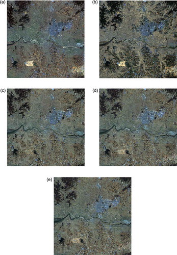
Figure 4. Images in their natural colors for the 11 March 2014 target date: (a) actual image obtained on the target date; (b) reference image acquired on 27 October 2013; (c) simulated image without NDVI and the reference image; (d) simulated image using NDVI; (e) simulated image using NDVI and the reference image.

The R² statistics of multilinear regression with the aid of NDVI are shown in Table 4. The R² maxima, minima, and means slightly increased, whereas the Stds and variances decreased compared with the first case. In addition, the at-sensor radiance was computed using Equation (8). The simulated images are shown in their natural colors in Figures 3(d) and 4(d).

Table 4. R² statistics of multilinear regression with the aid of NDVI.

Target date	Category	Band
		1	2	3	4	5	7
22 September 2006	Maximum	0.965	0.978	0.978	0.979	0.962	0.973
	Minimum	0.243	0.152	0.064	0.103	0.033	0.033
	Mean	0.849	0.828	0.811	0.872	0.609	0.670
	Std	0.056	0.078	0.096	0.068	0.164	0.137
	Variance	0.003	0.006	0.009	0.005	0.027	0.019
11 March 2014	Maximum	0.965	0.978	0.978	0.978	0.962	0.973
	Minimum	0.244	0.142	0.063	0.116	0.034	0.030
	Mean	0.857	0.836	0.828	0.877	0.607	0.680
	Std	0.048	0.077	0.091	0.066	0.167	0.140
	Variance	0.002	0.006	0.008	0.004	0.028	0.020

Table 5 shows the R² statistics of multilinear regression when NDVI and a reference image were used. As shown, compared with the cases in which a reference image was not used, the R² maxima and means slightly increased. Meanwhile, the Stds and variances of R² remained very small, which indicates that the regression model is reliable for estimating the simulated pixel values. Equation (8) was derived from this step and was used to generate the simulated pixel values. The simulated images acquired on 22 September 2006 and 11 March 2014 are shown in their natural colors in Figures 3(e) and 4(e), respectively.

Table 5. R² statistics of multilinear regression with the aid of NDVI and a reference image.

Target date	Category	Band
		1	2	3	4	5	7
22 September 2006	Maximum	0.976	0.981	0.984	0.979	0.962	0.978
	Minimum	0.230	0.152	0.064	0.103	0.033	0.033
	Mean	0.850	0.829	0.812	0.870	0.609	0.670
	Std	0.056	0.079	0.097	0.073	0.165	0.138
	Variance	0.003	0.006	0.009	0.005	0.027	0.019
11 March 2014	Maximum	0.982	0.987	0.987	0.990	0.977	0.984
	Minimum	0.245	0.142	0.064	0.118	0.034	0.030
	Mean	0.860	0.842	0.831	0.880	0.618	0.680
	Std	0.050	0.079	0.092	0.067	0.173	0.145
	Variance	0.002	0.006	0.008	0.004	0.030	0.021

Quality assessment of simulated images

In the simulated image on 22 September 2006, it is evident that two roads – one in the upper area; the other in the lower left (denoted as red rectangles in Figure 3(a)) – are not clearly shown without the aid of the reference image (denoted as red rectangles in Figure 3(c)). This is on account of the changes in land cover over the long time period in which the input images were acquired. With the reference image applied, these errors were nearly overcome (see Figure 3(e)). To evaluate the quality of the simulated images, SCM was used to compare the similarities between the simulated and actual images; that is, the Landsat 5 TM image acquired on 22 September 2006 (Figure 3(a)) and the Landsat 8 image obtained on 11 March 2014 (Figure 4(a)), respectively. Histograms of R, which are used to detect changes in SCM, are shown in Figure 5. The percentage of pixels with an R > 0.99, which can represent a state of no change, increased significantly when NDVI was applied and slightly increased when a reference image was used. On the contrary, the percentage of pixels with an R of less than 0.95, which can represent different land cover features in the two images, decreased.

Figure 5. Histogram of correlation coefficients between the simulated and actual images acquired on (a) 22 September 2006 and (b) 11 March 2014.

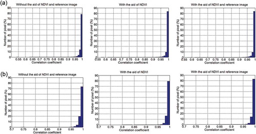
Table 6 shows the statistics of R with the mean of R being very high (greater than 0.99) in all cases: without the aid of the NDVI or a reference image (case 1); with the aid of NDVI (case 2); and with the aid of NDVI and a reference image (case 3). With the aid of NDVI, it slightly increased from 0.9912 to 0.9922 for the 2006 simulation, and from 0.9917 to 0.9930 for the 2014 simulation. When the reference image was applied, the mean of R increased to 0.9925 and 0.9936 for the 2006 and 2014 simulations, respectively. R ranged from approximately 0.54 to 1, and from approximately 0.74 to 1, for the 2006 and 2014 simulations, respectively. The standard deviations of R were very small and slightly decreased when NDVI and a reference image were applied. These very small values indicate that R tended to be close to the mean. With the aid of NDVI and a reference image, the percentage of pixels with an R > 0.99 significantly increased; meanwhile, the percentage of pixels with an R < 0.95 decreased. As shown in Table 6 and Figure 5(a), in the 2006 simulation without the aid of NDVI and a reference image, more than 78% of the pixels had an R > 0.99, and approximately 92% of the pixels had an R > 0.98. These pixels could be considered similar. Only slightly more than 2% of the pixels had an R < 0.95; these pixels can be considered very different. With the aid of NDVI, more than 83% of the pixels had an R > 0.99, approximately 93% of the pixels had an R > 0.98, and approximately 2% of the pixels had an R < 0.95 (Figure 5(a)). When applying the reference image, the percentage of pixels with an R greater than 0.99 and 0.98 increased slightly; that is, 84.3% and 93.23%, respectively. Meanwhile, the percentage of pixels with R value less than 0.95 was slightly decreased.

Table 6. Correlation coefficient statistics of the actual and simulated images.

Category	22 September 2006						11 March 2014
	Overall			Man-made area			Overall			Man-made area
	Case 1	Case 2	Case 3	Case 1	Case 2	Case 3	Case 1	Case 2	Case 3	Case 1	Case 2	Case 3
Mean	0.9912	0.9922	0.9925	0.9875	0.9894	0.9907	0.9917	0.9930	0.9936	0.9922	0.9937	0.9961
Std	0.0159	0.0148	0.0147	0.0241	0.0210	0.0206	0.0084	0.0065	0.0060	0.0095	0.0073	0.0043
Maximum	1.0000	1.0000	1.0000	1.0000	1.0000	1.0000	1.0000	1.0000	1.0000	1.0000	1.0000	1.0000
Minimum	0.5367	0.5714	0.5884	0.6713	0.7364	0.7392	0.7371	0.8025	0.8368	0.7538	0.8025	0.8899
R	Percentage of pixels (%)
>0.99	78.45	83.64	84.30	73.48	77.26	81.01	74.75	79.86	82.05	77.32	83.15	93.25
>0.98	91.79	92.88	93.23	85.04	87.89	89.39	93.64	95.83	96.63	92.42	95.27	98.94
<0.95	2.15	2.09	1.98	6.09	4.77	3.96	0.64	0.16	0.12	0.79	0.27	0.05

The same pattern was revealed in the 2014 simulation (see Table 6 and Figure 5(b)). When using the NDVI as a predictor, the percentage of pixels with an R > 0.98 increased from 93.64% to 95.83%, whereas the percentage of pixels with an R < 0.95 decreased to nearly 0%. This pattern also appeared when both NDVI and a reference image were applied, which indicates that their application improves the quality of the simulated images (although the reference image was only applied to man-made areas). Pixels with an R of less than 0.95 predominantly appeared in an area that significantly changed during the period in which the input images were acquired.

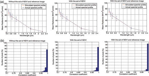
Figures 6 and 7 show the profiles of the mean spectral radiance and histograms of R in man-made areas without using NDVI or a reference image (Figures 6 and 7 (on the left in both)), with the aid of NDVI (Figures 6 and 7 (in the middle in both)), and with the aid of NDVI and a reference image (Figures 6 and 7 (on the right in both)). It is clear that when using a reference image to discard changed pixels in the man-made area, the percentage of pixels with R > 0.99 significantly increased. This led to an increase in the mean values and the percent of pixels with R > 0.98. The minima of R also substantially increased, whereas the percentage of pixels with R < 0.95 significantly dropped. NDVI also helped improve the quality of the simulated image in man-made areas. For the 2006 simulated image, the number of pixels with an R > 0.99 significantly increased from over 73% to above 77% when using NDVI alone and to above 81% when both NDVI and a reference image were used. The minimum value of R increased from 0.6713, the value when neither NDVI nor a reference image was used, to over 0.73 when both NDVI and a reference image were used. The mean value also increased slightly from 0.9875 to over 0.99 (Table 6). This pattern was additionally found in the 2014 simulation. In man-made areas, the percentage of pixels with an R > 0.99 significantly increased from 77.32% to 93.25% when NDVI and a reference image were applied. In addition, the number of pixels with an R < 0.95 decreased from 0.79 to 0.05. This shows that using NDVI and a reference image can significantly improve the image simulation quality in areas where they are applied. It is additionally apparent that land cover changes reduce the simulation quality.

Figure 6. Spectral profile (top) and histogram of correlation coefficients (bottom) for man-made areas with the 22 September 2006 target date.

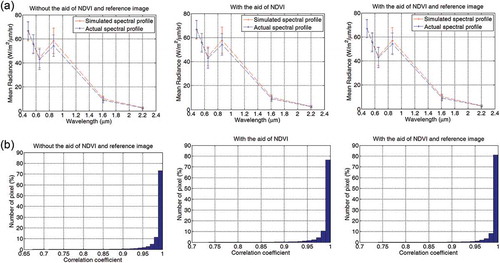
Figure 7. Spectral profile (top) and histogram of correlation coefficients (bottom) for man-made areas with the 11 March 2014 target date.

The RRMSE of the pixel radiance for each band of the simulated and actual images were calculated using Equation (9); they are shown in Table 7. Overall, the RRMSE slightly decreased when NDVI and a reference image were applied. The RRMSE values of bands 1 and 2 were the smallest. They were approximately 0.05 for band 1 and approximately 0.09 for band 2 for the 2006 simulation and approximately 0.1 and 0.08, respectively, for the 2014 simulation. The red and near infrared (NIR) bands (bands 3 and 4, respectively) had higher RRMSE values compared with those of bands 1 and 2, which was the result of the high sensitivity of these bands to changes in vegetation health. Consequently, the impact of changes in land cover was greater on these bands. It can also be seen that the RRMSE values of bands 5 and 7 were greater than those for the other spectral regions with the maximum value 0.4350 for band 7, which may be owing to the sensitivity to moisture of these bands; the errors likely resulted from a lack of atmospheric parameter measurements for water vapor content. Moreover, the radiance values of these bands were quite small; thus, a small difference between the actual and simulated values also resulted in a large RRMSE value.

Table 7. RRMSE value of pixel radiance for each band.

		Band
		1	2	3	4	5	7
Target date	Wavelength (µm)	0.485	0.569	0.660	0.840	1.676	2.223
22 September 2006	Case 1	0.0588	0.0945	0.2053	0.1535	0.3624	0.4350
	Case 2	0.0531	0.0879	0.1976	0.1429	0.3566	0.4033
	Case 3	0.0535	0.0872	0.1946	0.1387	0.3525	0.4006
11 March 2014	Case 1	0.1098	0.0878	0.1228	0.1325	0.1953	0.2815
	Case 2	0.1056	0.0775	0.1037	0.1292	0.1807	0.2583
	Case 3	0.1004	0.0727	0.0964	0.1219	0.1688	0.2460

Discussion

Compared to other simulation methods such as Guanter, Segl, and Kaufmann (2009), Zhao et al. (2013), the proposed method likewise provided good results. The difference in radiance between simulated and original image was up to 10–15% in Guanter, Segl, and Kaufmann (2009); and in Zhao et al. (2013), RRMSE was smaller than 0.1 for VNIR bands and was close to 1 for bands around 2.3 µm; while in our study, minimum RRMSE was 0.05 for band 1 (0.485 µm) and the maximum was 0.4250 for band 7 (2.223 µm). In addition, the main benefits of the proposed model are the cost-effectiveness and the simplicity, since it relies on the open data sources and does not require the results from complicated radiative transfer codes such as MODTRAN and LOWTRAN.

However, the quality of the simulated images derived using the proposed approach is sensitive to changes in land cover during the period in which the input satellite images were acquired. This is a limitation of multitemporal-based approaches. Note that the area of study is a developing area mainly covered by agricultural land. Therefore, land cover typically varies month by month and year by year. Even water, which can be typically expected to be a stable feature, undergoes alterations. Although, land cover change is hard to be predicted especially the nonstationary change patterns (Estoque and Murayama 2014), its effects on image simulation can be minimized by applying NDVI and a reference image. NDVI on the target date can be interpolated from the NDVIs for the same season, or replaced with the NDVI on a date close to the target date if available. Unfortunately, appropriate reference images for the geographic features that significantly change over short periods of time are not easy to obtain, especially in agricultural areas, where farmland is bare after harvest, and conversely in growing season bare land can be covered by green plants. Consequently, selecting reference images for agricultural land must consider the lifecycle of the crops. This task is easier for man-made areas, for rapidly urbanizing areas, where the land cover can change significantly over a short span of time, the reference image can be any image acquired within the same year in which the simulated image is generated; however, for urbanized areas that change very slowly, a 1- or 2-year lag between reference image and simulated image is acceptable. In addition to using reference image and NDVI to reduce the effect of land cover changes, we attempted to exclude some images that were acquired in different seasons. For the simulation on 22 September 2006, images obtained in March, April, and November were excluded from the dataset. Thirty-eight images were employed in the simulation. Consequently, the quality of simulated images slightly improved in comparison with using the full dataset. For example, the percentage of pixels with R > 0.99 increased from 83.64% to 84.21% when NDVI was applied. However, if only images acquired from March to May were used for the 2014 simulation, the results were much worse compared with when using the full dataset. This was because there were only 25 remaining images if we excluded images acquired from June to November; among them, there were several images with cloud contamination. Therefore, they were insufficient for enabling a satisfactory relationship between the predictors and pixel value. In addition, the input dataset contains many images obtained during a long period of time using different sensor types; hence, spatial co-registration errors of one or two pixels are possible, which could also decrease the accuracy of the output results.

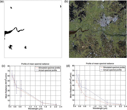
As shown in Figure 3(c)–(e), the color of part of the river in the middle of the simulated image differs from that in the actual image. This discrepancy was caused by the wide fluctuation of water levels in that part of the river. A dam exists in the middle of the river; when closed, the downriver water level is lower and the turbidity may be increased because of the slow water flow. Therefore, the color was lighter than that of the actual image, which was obtained on the date the dam was opened. Unfortunately, the respective images in the dataset are primarily those with the dam closed. Consequently, the color of this part of the image is also lighter in the simulated image. This phenomenon was reduced in the 2014 simulated image (Figure 4(c) and (d)) when the dam was closed. This effect could be resolved by applying a reference image, as in the case of the man-made area. However, the dataset includes no images that were acquired when the dam was open that were near the target dates; hence, a reference image was not applied for this area. To overcome this problem, we attempted to use the shuttle radar topography mission (SRTM) water body data (SWBD) (Figure 8(a)), which is a geographical dataset published by the US National Aeronautics and Space Administration (NASA) (USGS 2014) that encodes high-resolution worldwide coastal outlines in vector format. The pixel value within the river’s boundary was replaced with that of the reference image (obtained on 12 October 2005). The result is shown in Figure 8(b); the spectral profiles of the mean radiance of the replaced pixels are shown in Figure 8(c) and (d). As shown in the figures, the result when considering the SWBD is even worse than when not considering the SWBD because the reference image was acquired on a date the dam was closed. However, this problem can be overcome if we have images obtained when the dam was open, or when tidal information is available.

Figure 8. Image simulation with and without SWBD for the target date of 22 September 2006: (a) SWBD; (b) simulated image with a reference image and SWBD; (c) mean spectral radiance profile without SWBD; and (d) mean spectral radiance profile with SWBD.

However, the quality of the simulated images obtained from the proposed approach can be substantially improved by applying a higher-quality NDVI and a reference image (i.e., an interpolated NDVI that is correlated more to the real NDVI, and a reference image that is quite similar to the image on the target date). The result can also be more accurate if the acquisition dates of the input dataset are close to the target date (i.e., a high temporal resolution), or when the dynamics of the geographical features in the application area are slow during the total time of the input data acquisition. The accuracy of the predictors additionally has an effect on the simulation results. Initially, various parameters were used in the model, such as land surface temperature (LST) and aerosol optical thickness (AOT). However, these parameters were estimated from many factors. Errors can exist in these estimations. Furthermore, LST on the simulation date is not known; although it can be interpolated from LST on the proximate dates, the errors cannot be eliminated. Moreover, these errors can introduce more errors in the final results of the model. Consequently, the results when applying LST and AOT are very poor (the percentages of pixels with R > 0.99 in cases of applying AOT and LST were below 70%). Therefore, these factors were not used in the model. Optimal parameters that have significant effects on the radiance measured by sensors may improve the simulation quality. In this study, we additionally attempted to use the map of the meteorological parameters interpolated from the values measured by the two ground stations near the study area using inverse distance squared method (Nalder and Wein 1998). However, the results were almost the same as those from using the mean values of the two ground stations. Therefore, for simplification and to reduce the processing time, the average values were used for an entire 24 km × 24 km area. Nevertheless, spatially distributed meteorological parameters, which can be interpolated from a sufficient number of stations, could perhaps improve the simulation results.

Shadow effects were also considered in this study. If a location in a simulated image did not have a shadow, then only nonshadow pixels in the input dataset were selected for the simulation process. This selection mode was also conducted for shadow pixels. However, the study area was quite flat. Hence, there were only a few shadow pixels present in the images. Consequently, the result was almost the same as when shadow effects were not considered. However, this may have been an important factor affecting the quality of the simulated images in mountainous areas and in the simulation of a high-spatial-resolution image.

Owing to its flexibility, the proposed approach can be used for a simulation of multispectral images at any spatial and spectral resolution under diverse natural environments and atmospheric conditions. Currently, nearly open data sources provide satellite images with spatial resolutions of 30 m or coarser. However, in the future, when super-high-resolution satellite sensors are launched, finer-resolution satellite images will become accessible and will thereby advance the capabilities and quality of our approach.

Conclusion

The objective of this study was to develop a simple model for image simulation based on a temporal correlation of multitemporal satellite images and weather conditions that can be easily accessed through open data sources. This model was tested to generate simulated images that were acquired on the study site on select dates. Various comparisons between the simulated and actual images were conducted, and satisfactory results were attained. These results show that the simulated images were quite similar to the actual images; the percentage of pixels with correlation coefficients above 0.98 when using NDVI and a reference image were more than 93% and more than 96% for the simulations conducted on two different weather conditions. Because the proposed approach is multitemporal-based, the quality of the simulated images generated by the proposed model is primarily affected by land cover changes. However, this effect can be significantly reduced by applying NDVI as a predictor, using a reference image to exclude changed pixels, or collecting input images acquired near the target date of the simulation. The quality of the proposed model can be greatly improved if applied to areas with slight changes or if high temporal satellite images are used, thereby resulting in the acquisition dates of the input dataset being close to the target date. Shadow effects may also be an important factor that requires consideration when simulating mountainous areas and high-spatial-resolution images.

Given its flexibility, in addition to simulating multispectral image, the proposed approach can be recommended for simulating hyperspectral image at any spatial and spectral resolution for diverse natural environments and atmospheric conditions. Moreover, in the future, when more super-high-resolution satellite sensors are launched, finer-resolution satellite images will become accessible and will therefore advance the capabilities and quality of our approach. Although the results generated by our model are quite good, further research is needed to improve its accuracy and applicability in diverse areas. Finding optimal nonlinear regression equations or other predictors to obtain the best temporal correlation is likewise important for future studies.

Disclosure statement

No potential conflict of interest was reported by the authors.

Additional information

Funding

This research was supported by the Basic Science Research Program through the National Research Foundation of Korea (NRF) funded by the Ministry of Education [grant number NRF-2013R1A1A2007582].

References

- Berk, A., G. P. Anderson, L. S. Bernstein, P. K. Acharya, H. Dothe, M. W. Matthew, and S. M. Adler-Golden, et al. 1999. “MODTRAN4 Radiative Transfer Modeling for Atmospheric Correction.” In Proceeding of SPIE 3756: Optical Spectroscopic Techniques and Instrumentation for Atmospheric and Space Research III. doi:10.1117/12.366388.
- Blaschke, T. 2010. “Object Based Image Analysis for Remote Sensing.” ISPRS Journal of Photogrammetry and Remote Sensing 65 (1): 2–16. doi:10.1016/j.isprsjprs.2009.06.004.
- Blonski, S., M. H. Lean, J. L. Jensen, R. B. Crosier, and M. S. Schlein. 1997. “Computational Prototyping of the Chemical Imaging Sensor.” In Proceedings of SPIE 3118: Imaging Spectrometry III. doi:10.1117/12.278937.
- Cao, C., S. Blonski, R. Ryan, J. Gasser, V. Zanoni, and J. Jenner. 1999. “Synthetic Scene Generation of the Stennis V&V Target Range for the Calibration of Remote Sensing Systems.” Proceedings of the International Symposium on Spectral Sensing Research, Las Vegas, NV, 31 October–4 November
- Carl, S., D. S. Joseph, and R. John. 1993. “Use of Lowtran-Derived Atmospheric Parameters in Synthetic Image Generation Models.” In Proceedings of SPIE 1938: Recent Advances in Sensors, Radiometric Calibration, and Processing of Remotely Sensed Data, 294–307. doi:10.1117/12.161555.
- Carvalho Júnior, O. A., R. F. Guimarães, A. R. Gillespie, N. C. Silva, and R. A. T. Gomes. 2011. “A New Approach to Change Vector Analysis Using Distance and Similarity Measures.” Remote Sensing 3 (11): 2473–2493. doi:10.3390/rs3112473.
- Chen, S., L. Chen, Y. Liu, and X. Li. 2013. “Experimental Simulation on Mixed Spectra of Leaves and Calcite for Inversion of Carbonate Minerals from EO-1 Hyperion Data.” GIScience & Remote Sensing 50 (6): 690–703. doi:10.1080/15481603.2013.866792.
- Chen, X., Z. Su, Y. Ma, K. Yang, and B. Wang. 2013. “Estimation of Surface Energy Fluxes under Complex Terrain of Mt. Qomolangma over the Tibetan Plateau.” Hydrology and Earth System Sciences 17: 1607–1618. doi:10.5194/hess-17-1607-2013.
- Estoque, R. C., and Y. Murayama. 2014. “A Geospatial Approach for Detecting and Characterizing Non-Stationarity of Land-Change Patterns and Its Potential Effect on Modeling Accuracy.” GIScience & Remote Sensing 51 (3): 239–252. doi:10.1080/15481603.2014.908582.
- Gascon, F., J.-P. Gastellu-Etchegorry, and M.-J. Lefevre. 2001. “Radiative Transfer Model for Simulating High-Resolution Satellite Images.” IEEE Transactions on Geoscience and Remote Sensing 39 (9): 1922–1926. doi:10.1109/36.951083.
- Gates, D. M. 1980. Biophysical Ecology. New York: Springer-Verlag.
- Gill, K. M. 2012. “CASTING SHADOWS: Shading Digital Elevation Models Using Ray Tracing.” Rivier University Academic Journal 8 (1): 1–15.
- Guanter, L., K. Segl, and H. Kaufmann. 2009. “Simulation of Optical Remote-Sensing Scenes with Application to the EnMAP Hyperspectral Mission.” IEEE Transactions on Geoscience and Remote Sensing 47 (7): 2340–2351. doi:10.1109/TGRS.2008.2011616.
- Gueymard, C. 1995. SMARTS2, a Simple Model of the Atmospheric Radiative Transfer of Sunshine: Algorithms and Performance Assessment. USA: Rep. FSEC-PF-270-95 Florida Solar Energy Center.
- Guisan, A., N. E. Zimmermann, J. Elith, C. H. Graham, S. Phillips, and A. T. Peterson. 2007. “What Matters for Predicting the Occurrences of Trees: Techniques, Data, or Species’ Characteristics?” Ecological Monographs 77 (4): 615–630. doi:10.1890/06-1060.1.
- Hocking, R. R. 1976. “The Analysis and Selection of Variables in Linear Regression.” Biometrics 32 (1): 1–49.
- Hook, S. J., J. J. Myers, K. J. Thome, M. Fitzgerald, and A. B. Kahle. 2001. “The MODIS/ASTER Airborne Simulator (MASTER) – a New Instrument for Earth Science Studies.” Remote Sensing of Environment 76 (1): 93–102. doi:10.1016/S0034-4257(00)00195-4.
- Ju, J., and D. P. Roy. 2008. “The Availability of Cloud-Free Landsat ETM+ Data over the Conterminous United States and Globally.” Remote Sensing of Environment 112 (3): 1196–1211. doi:10.1016/j.rse.2007.08.011.
- Kaufman, Y. J. 1993. “Aerosol Optical Thickness and Atmospheric Path Radiance.” Journal of Geophysical Research 98 (D2): 2677–2692. doi:10.1029/92JD02427.
- Kim, S., Y. Eo, B. Lee, I. Jang, and S. Han. 2013. “Remote Sensed Image Simulation Methodology.” Journal of Next Generation Information Technology (JNIT) 4 (8): 111–117.
- Korean Meteorological Administration. 2015. “Climate of Korea.” Accessed May 1. http://web.kma.go.kr/eng/biz/climate_01.jsp
- Kumar, L., and A. K. Skidmore. 2000. “Radiation-Vegetation Relationship in a Eucalyptus Forest.” Photogrammetric Engineering & Remote Sensing 66 (2): 193–204.
- Kumar, L., A. K. Skidmore, and E. Knowles. 1997. “Modelling Topographic Variation in Solar Radiation in a GIS Environment.” International Journal of Geographical Information Science 11 (5): 475–497. doi:10.1080/136588197242266.
- Lin, F.-C., L.-K. Chung, C.-J. Wang, W.-Y. Ku, and T.-Y. Chou. 2013. “Storage and Processing of Massive Remote Sensing Images Using a Novel Cloud Computing Platform.” GIScience & Remote Sensing 50 (3): 322–336. doi:10.1080/15481603.2013.810976.
- Nalder, I. A., and R. W. Wein. 1998. “Spatial Interpolation of Climatic Normals: Test of a New Method in the Canadian Boreal Forest.” Agricultural and Forest Meteorology 92 (4): 211–225. doi:10.1016/S0168-1923(98)00102-6.
- Nathans, L. L., F. L. Oswald, and N. Kim. 2012. “Interpreting Multiple Linear Regression: A Guidebook of Variable Importance.” Practical Assessment, Research & Evaluation 17 (9): 1–19.
- Ouaidrari, H., and E. F. Vermote. 1999. “Operational Atmospheric Correction of Landsat TM Data.” Remote Sensing of Environment 70 (1): 4–15. doi:10.1016/S0034-4257(99)00054-1.
- PRA. 1998. GCI Toolkit Manual. San Diego, CA: Photon Research Associates.
- Qin, Z., A. Karnieli, and P. Berliner. 2001. “A Mono-Window Algorithm for Retrieving Land Surface Temperature from Landsat TM Data and Its Application to the Israel-Egypt Border Region.” International Journal of Remote Sensing 22: 3719–3746. doi:10.1080/01431160010006971.
- Rouse, J. W., R. H. Haas, J. A. Schell, and D. W. Deering. 1974. “Monitoring Vegetation Systems in the Great Plains with ERTS.” In Third ERTS Symposium, 309–317, Washington, DC: NASA SP-351, NASA.
- Sabel, D., Z. Bartalis, W. Wagner, M. Doubkova, and J.-P. Klein. 2012. “Development of a Global Backscatter Model in Support to the Sentinel-1 Mission Design.” Remote Sensing of Environment 120: 102–112. doi:10.1016/j.rse.2011.09.028.
- Salisbury, J. W. 1998. Spectral Measurements Field Guide. Defence Technology Information Centre, Report No. ADA362372. Fort Belvoir, VA: Earth Satellite Corporation.
- Schill, S. R., J. R. Jensen, G. T. Raber, and D. E. Porter. 2004. “Temporal Modeling of Bidirectional Reflection Distribution Function (BRDF) in Coastal Vegetation.” GIScience & Remote Sensing 41 (2): 116–135. doi:10.2747/1548-1603.41.2.116.
- Schläpfer, D., and J. Nieke. 2005. “Operational Simulation of at Sensor Radiance Sensitivity using the MODO/MODTRAN Environment.” In Proceedings of the 4th EARSeL Workshop on Imaging Spectroscopy, edited by B. Zagajewski, M. Sobczak, and M. Wrzesień, Warsaw, April 27–29, 611–619.
- Schott, J. R., S. D. Brown, R. V. Raqueño, H. N. Gross, and G. Robinson. 1999. “An Advanced Synthetic Image Generation Model and its Application to Multi/Hyperspectral Algorithm Development.” Canadian Journal of Remote Sensing 25 (2): 99–111. doi:10.1080/07038992.1999.10874709.
- Stark, R. 1993. “Synthetic Image Generator Model: Application of View Angle Dependent Reflectivity Components and Performance Evaluation in the Visible Region.” Master’s thesis of Science in the Center for Imaging Science, College of Imaging Arts and Sciences of the Rochester Institute of Technology, New York.
- USGS. 2014. “NASA Shuttle Radar Topography Mission Water Body Data Shapefiles & Raster Files.” Accessed August 1, 2015. https://lpdaac.usgs.gov/products/measures_products_table/srtmswbd
- Vermote, E. F., D. Tanre, J. L. Deuze, M. Herman, and J.-J. Morcette. 1997. “Second Simulation of the Satellite Signal in the Solar Spectrum, 6S: An Overview.” IEEE Transactions on Geoscience and Remote Sensing 35 (3): 675–686. doi:10.1109/36.581987.
- Zhao, H., C. Jiang, G. Jia, and D. Tao. 2013. “Simulation of Hyperspectral Radiance Images with Quantification of Adjacency Effects over Rugged Scenes.” Measurement Science and Technology 24 (12): 1–12. doi:10.1088/0957-0233/24/12/125405.