Spatiotemporal changes of urban impervious surface area and land surface temperature in Beijing from 1990 to 2014

Abstract

This study examined changes in urban expansion and land surface temperature in Beijing between 1990 and 2014 using multitemporal TM, ETM+, and OLI images, and evaluated the relationship between percent impervious surface area (%ISA) and relative mean annual surface temperature (RMAST). From 1990 to 2001, both internal land transformation and outward expansion were observed. In the central urban area, the high-density urban areas decreased by almost 7 km², while the moderate- and high-density urban land areas increased by 250 and 90 km², respectively, outside of the third ring road. From 2001 to 2014, high-density urban areas between the fifth and sixth ring roads experienced the greatest increase by more than 210 km², and RMAST generally increased with %ISA. During 1990–2001 and 2001–2014, RMAST increased by more than 1.5 K between the south third and fifth ring roads, and %ISA increased by more than 50% outside of the fifth ring road. These trends in urban expansion and RMAST over the last two decades in Beijing can provide useful information for urban planning decisions.

Keywords:

• urban expansion
• urban impervious surface
• mean annual surface temperature
• Beijing

1. Introduction

Urban areas cover 0.5% of Earth’s terrestrial surface, and an increasing number of people are living in urban areas as cities expand, particularly in developing countries. Anthropogenic activities have led to numerous problems, such as air pollution and water pollution. In addition, the development of urban heat islands (UHI), which refers to the phenomenon of increased surface temperatures in urban areas compared to surrounding areas, is a major impact of urbanization (Weng 2009). Moreover, UHI causes weather anomalies, a deterioration of the living environment, increases in energy consumption, and even a rise in mortality (Wong, Paddon, and Jimenez 2013; Rizwan, Dennis, and Liu 2008; Shepherd and Burian 2003).

Remote sensing observations of land surface temperature (LST) have been widely used to research surface urban heat islands (SUHI) in many metropolises (Yang, Ren, and Liu 2013; Li, Zhang, and Kainz 2012; Gaffin et al. 2008; Li, Tang et al. 2013; Streutker 2002). In addition, multitemporal LST data have been used to extract parameters of annual and diurnal LST cycles. Gottsche and Olesen (2001) used a diurnal temperature model to describe thermal performance and to extract land surface properties at a spatial resolution of 5 km. At a finer resolution, Bechtel (2012) used Landsat 5 and 7 data and an annual temperature model (ATM) to obtain the mean annual surface temperature (MAST), and the yearly amplitude of surface temperature (YAST), which can be used to detect the urban LST variability without taking urban heterogeneity into consideration (Weng and Fu 2014).

Many studies have described the relationship between changes in land use/land cover (LULC) and LST, confirming that hotspots are mainly located in areas dominated by bare soil and building materials, while parks are 1–3 K, and sometimes more than 5 K, cooler than their urban surroundings (Sun et al. 2012; Cao et al. 2010; Li, Zhang, and Kainz 2012; Liu and Weng 2009; Chen et al. 2006). In addition, rapid urban expansion, characterized by an increase in impervious surfaces (e.g., buildings and roads), and a decrease in vegetation (e.g., grass and agricultural land), has significantly increased LST in recent decades (Ding and Shi 2013; Kaufmann et al. 2007; Amiri et al. 2009). However, the LULC classification is a “hard classification” algorithm, and the accuracy of LULC is relatively low because of mixed pixel problems (Weng and Lu 2009; Li, Lu et al. 2013). Moreover, Ridd (1995) maintained that urban components fractions should be applied to better understand the urban composition.

The vegetation-impervious surface-soil (V-I-S) model is a major conceptual model for remote sensing analysis of urban landscapes (Ridd 1995). The model assumes that urban land cover is a linear combination of three components: vegetation, impervious surface, and soil. It is a continuum landscape model that can effectively define standardized urban landscape components at the sub-pixel level in both temperate and tropical cities (Tang et al. 2012; Phinn et al. 2002; Weng and Lu 2009). Additionally, sub-pixel-based approach has the potential to detect small changes of urban land covers (Zhang, Chen, and Lu 2015). Among the three components of the V-I-S model, impervious surface is the most stable indicator of the degree of urbanization with the least seasonal variability (Weng and Lu 2009). Several methods, such as linear spectral mixture analysis (LSMA) and normalized spectral mixture analysis (NSMA) (Wu and Murray 2003; Wu 2004), have been proposed to extract the percent impervious surface area (%ISA) in mixed pixels based on the V-I-S model. In addition, previous studies have shown that %ISA has a stronger linear relationship to LST than other urban components and urbanization exponents, such as vegetation fraction (f_V) and normalized difference build-up index (Weng and Lu 2008; Yuan and Bauer 2007; Zhang, Odeh, and Han 2009; Zhang et al. 2009; Xu, Lin, and Tang 2013).

The main objectives of this study are (1) to analyze the spatiotemporal changes of MAST and %ISA in Beijing between 1990 and 2014, and (2) to examine the relationship between MAST and %ISA to understand the influence of urban components on MAST. To remove the effect of global warming (IPCC 2014), we established a forest mountain area as a reference area and used the MAST relative to this reference area (RMAST) to analyze the thermal environment of the study area. Landsat data have medium spatial resolution (30 m), a long-term time span, and contain both visible-near infrared and thermal infrared bands that can be used to monitor LST and %ISA changes (Cai, Du, and Xue 2011; Li, Tang et al. 2013; Powell et al. 2008; Torbick and Corbiere 2015; Weng 2012). Thus, all analyses in the presented research are conducted using Landsat data.

2. Study area and data

2.1. Study area

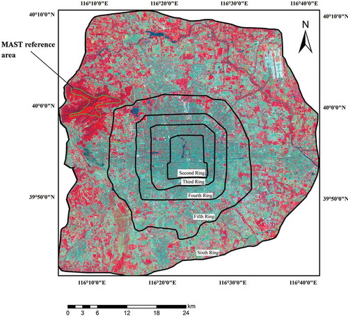
Beijing is located in the northwest region of the North China Plain (39°28′–41°25′N; 115°25′–117°30′E; see Figure 1). It covers an area of more than 16,800 km², with a mountainous region in the west. In addition, Beijing has a warm-temperate, continental monsoon climate. As the capital city of China, Beijing has experienced accelerated urbanization since the 1990s, driven by rapid economic development. In 2012, the total population of the city was approximately 20 million and the GDP reached 1600 billion yuan (US$252 billion) (Beijing Statistics Bureau 2012). Beijing is divided into multiple ring roads, and the area enclosed by the sixth ring road was selected as our study area (Figure 1).

Figure 1. Area enclosed by the sixth ring road obtained from TM standard false color composite images (2009/9/22; bands 4, 3, and 2; spatial resolution of 30 m) overlain by vector data of the second, third, fourth, fifth, and sixth ring roads. For full color versions of the figures in this paper, please see the online version.

2.2. Data and preprocessing

Cloud-free Landsat images from three time periods (1989–1992, 2000–2002, and 2013–2015) were obtained from the U.S. Geological Survey Earth Explorer (USGS 2015). There were 38, 48, and 56 images from the three periods, respectively (Table A1). Both level 2 products and land surface reflectance products for Landsat 4, 5, 7, and 8 were obtained. All images used a Universal Transverse Mercator projection (datum WGS84, UTM Zone N50) and cloud cover was less than 30%.

3. Methods

3.1. Overview of methods

Data coverage of Beijing from Landsat 4, 5, 7, and 8 was used to analyze spatiotemporal changes in %ISA and RMAST and to assess urban growth (Figure 2). We also analyzed the relationship between changes in %ISA and RMAST.

Figure 2. Process flow of this study.

3.2. Calculation of %ISA

Following the V-I-S model developed by Ridd (1995), we assumed that each spectrum from a mixed pixel was a product of various endmember spectra from vegetation, soil, and impervious surfaces. NSMA was used to calculate fraction images (Wu 2004), the first step of the NSMA was using a normalization process to reduce the brightness variation of the urban land cover using Equation (1):

(1)

(2)

where is the normalized reflectance for band b in a pixel, R_b is the original reflectance for band b, is the average reflectance for that pixel, and N is the total number of bands. After the normalization, heterogeneous urban composition of each pixel was calculated using constrained LSMA method as follows:

(3)

(4)

where is the normalized reflectance for band b, is the fraction of endmember i, is the normalized reflectance of endmember i in band b, N is the number of endmembers, and e_b is the residual.

We used three images (1990261, 2001267, and 2014247, mainly from September (hence, early autumn)) to extract the %ISA. Images from other seasons were not used because (1) in winter the study area was covered with snow and %ISA could not be extracted from the images; (2) in summer the high vegetation fraction led to an underestimation of %ISA, especially in urban areas; and (3) in spring the green-up phases of different vegetation produced large variations in spectral patterns, resulting in an overestimation of soil and %ISA.

To extract %ISA, water pixels were first masked using the normalized difference water index (McFeeters 1996); 0.1 was selected as the threshold. A principal component (PC) transformation was then used to process the normalized spectrum of the Landsat images (Wu 2004), and three endmembers (vegetation, soil, and impervious surface) were identified from the PC1/PC2, PC1/PC3, and PC2/PC3 feature space. The normalized spectrum of the endmembers is shown in Figure 3.

Figure 3. The endmembers used to extract %ISA.

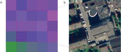
The %ISA results of the three time periods were validated using aerial photographs from 1991, IKONOS images from 2001, and QuickBird images from 2014, respectively. We used a stratified random sampling strategy to select 100 samples from each period, and the sampling unit was a 33 window of Landsat pixels. Relatively few samples with low %ISA were acquired in 1991 because the coverage from aerial photographs was limited. For each sample, the corresponding “true impervious surface” was digitized using high-resolution images and the impervious area was measured from the digitized map (Wu 2004) (Figure 4).

Figure 4. Sample validation site using a QuickBird image with a 3 × 3 sampling unit in 2009: (a) TM image (square with red line indicates a 3 × 3 sampling unit) and (b) QuickBird image (square with red line indicates the corresponding area of the 3 × 3 sampling unit).

3.3. Calculation of MAST

We used MAST derived from an ATM to measure the change in LST (Bechtel 2012). The ATM used a sine function to characterize the annual temperature, as follows:

(5)

where d is the day of the annual cycle (relative to the spring equinox). The annual cycle for each pixel was determined by three parameters: MAST and YAST are the mean and amplitude of the annual temperature cycle and θ is an optimal phase shift relative to the equinox. As 35 full coverage images are recommended to achieve effective ATM parameters (Bechtel 2012), images over multiple years were used in this study. Previous studies have used Landsat images from a 10-year span to drive the ATM, but Beijing is a highly dynamic city and land cover changes significantly affect the ATM parameters. Therefore, a balance must be reached between the number of years included and the land cover change. We aimed to obtain more than 30 cloud-free images over the fewest number of years. For the 1989–1992 period, we used images acquired over 4 years, while for the 2000–2003 and 2013–2015 periods, we used only the images acquired over 3 years because images were available from two sensors (Landsat 5 and Landsat 7 during 2001–2003 and Landsat 7 and Landsat 8 during 2013–2015). Scenes that were partly contaminated by cloud coverage were combined with full-coverage scenes to increase the image sampling. In addition, we assumed that the land cover did not change during the three time periods (1989–1992, 2000–2002, and 2013–2015). To mask the cloud cover pixels, a cloud product was employed for all Landsat images (Zhu and Woodcock 2012).

We used the revised single-channel algorithm to retrieve LST from the Landsat thermal infrared band. Landsat 8 has two thermal bands; we used TIRS-1 to retrieve LST because it is located in a lower atmospheric absorption region with high atmospheric transitivity values. After radiometric calibration, the radiometric brightness (L_s) was converted to a satellite brightness temperature (T_b) using the Planck function (Chander, Markham, and Helder 2009) as follows:

(6)

where T_b is the at-sensor brightness temperature in Kelvin, L_s is the radiometric brightness at the sensor aperture in , and and are the pre-launch calibration constants (K₁ = 607.76 and K₂ = 1260.56 K for Landsat 4 band 6 (L4B6); K₁ = 607.76 and K₂ = 1260.56 K for L5B6; K₁ = 666.09 and K₂ = 1282.71 K for L7B6; and K₁ = 774.89 and K₂ = 1321.08 K for Landsat TIRS-1). The brightness temperature was then converted to the LST using Equation (7) (Jimenez-Munoz et al. 2009):

(7)

where

(8)

(9)

(10)

(11)

(12)

where ε = 1 was the emissivity, and we used the brightness temperature to exclude the correlation between LST and %ISA. The parameters γ and δ are dependent on the Planck function, was 1290 , 1256, 1277 and 1324 K for band 6 of Landsat 4, 5, and 7 and Landsat 8 TIR-1, respectively, and the atmospheric function components, , , and , were calculated using the water vapor content, w, obtained from sounding data (University of Wyoming 2015).

After calculating MAST, we selected the mountainous in northwest region of the city as a reference area (Figure 1) and assigned the average MAST of the reference area as the reference MAST. Next, we defined the difference between MAST and the reference temperature as RMAST, which effectively excluded effects of global warming.

4. Results and discussion

4.1. Validation of %ISA estimation

The root-mean-square error (RMSE) and the correlation coefficient (R²) were used to evaluate the accuracy of %ISA estimates (Figure 5). The respective RMSE and R² were 11.47% and 0.92 in 1990, 13.24% and 0.93 in 2001, and 11.71% and 0.92 in 2014 (Table 1). Generally, %ISA was overestimated when the actual %ISA was <20%, and it was underestimated when the actual fraction was >80%, similar to results found in previous studies (Sexton et al. 2013; Wu 2004).

Figure 5. Residual analysis of impervious surface estimation.

Table 1. RMSE and R² between estimated %ISA and validation samples.

Year	R^2	RMSE (%)
1990	0.92	11.47
2001	0.93	13.24
2014	0.92	11.71

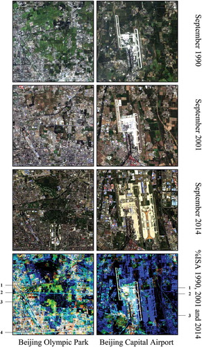
Although there were uncertainties associated with the extraction of %ISA, local dynamics were generally captured by the %ISA images and the local dynamics were exemplified by two sites: the Beijing Capital International Airport (BCIA) and the Beijing Olympic Park (BOP) (Figure 6). The %ISA remained at or near 100% (white patches in the button figures for both sites), such as the road labeled “4” for BOP and the first terminal of the airport labeled “1” for BCIA. Impervious areas developed between 1990 and 2001 were cyan patches, such as the road labeled “2” for BOP and the second terminal labeled “2” for BCIA. The cyan road in BOP was the north fifth ring road built in 2000, and the second terminal was built in 1999. The blue patches were the impervious areas built between 2001 and 2014, including the runways of the third terminal labeled “3” for BCIA. Areas with decreasing imperviousness were also observed (green and yellow patches), labeled “1” and “3” for BOP. These include areas that were impervious between 1990 and 2001 but became pervious in 2014 (yellow patches), and areas that were built-up and became impervious between 1990 and 2001, then became pervious before 2014 (green patches). The decrease in imperviousness for BOP was mainly due to the development of the Olympic Forest Park in 2007.

Figure 6. Development of Beijing Olympic Park (BOP) and Beijing Capital International Airport (BCIA). The first three images are true-color images, and the bottom images are composited of the impervious fraction from different periods (red is 1990, green is 2001, and blue is 2014).

4.2. Uncertainty of the MAST

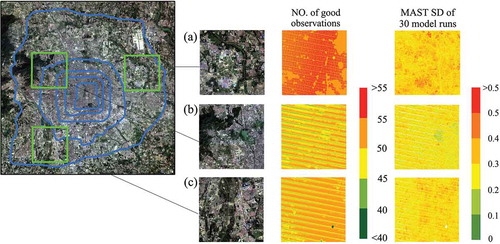
The number of cloud-free observations for each period is shown in Figure 7. In general, more than 40 cloud-free observations were obtained for the 2000–2002 and 2013–2015 periods and more than 30 cloud-free observations were obtained for the 1989–1992 period. We tested the uncertainty of MAST estimated by “35 cloud-free observations” for the following reasons: (1) “35 cloud-free observations” was recommended as the lowest number for the MAST estimation (Bechtel 2012), and (2) the number of cloud-free observations from the 1989–1992 period was around 35, which was the lowest among the three time periods used in this research. The data from the 2013–2015 period were used to test the uncertainty of “35 cloud-free observations” as we obtained the most cloud-free images during this time period. Three subregions (a, b, and c) were used to test the uncertainty (Figure 8), and 35 Landsat observations were randomly selected from all available observations for each pixel within the subregions. Next, the standard deviation (SD) of the 30 MASTs was used to measure the uncertainty of the MAST estimation. The subsets drawn from the 55 Landsat observations during 2013 and 2015 (Figure 8) were not entirely independent. Thus, the uncertainty measure was not perfect; however, it was deemed reasonable because the data were the only Landsat data we could acquire during this time period. It was notable that the number of cloud-free Landsat images was relatively low (< 40) in subregions b and c because of the gaps from Landsat 7 data (the green pixels in the “number of good observation” subfigures of Figure 8), and these pixels were not used in measuring the uncertainty. The spatial distribution of the SD for the 30 model runs of the three subregions are shown in Figure 8. The mean MAST SDs of the three subregions were 0.32, 0.26, and 0.29 K, respectively. Cropland had relatively high MAST SD (around 0.5 K), such as the cropland labeled “1” in subregion (a). In contrast, waterbodies had low MAST SD (around 0.2 K), such as the river labeled “1” in subregion (a) and the lake labeled “2” in subregion (b). Generally, these results indicated that “35 cloud-free observations” offered the potential for an accurate MAST calculation. Thus, the MAST of the three time periods (1989–1992, 2000–2002, and 2013–2015) acquired in this study could describe the MAST change over the last two decades.

Figure 7. Number of cloud-free Landsat observations for the three periods.

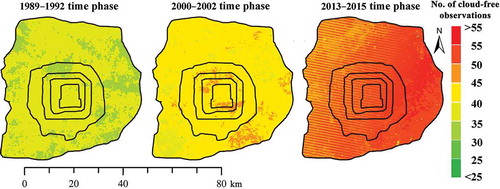
Figure 8. The MAST standard deviations of the three tested subregions.

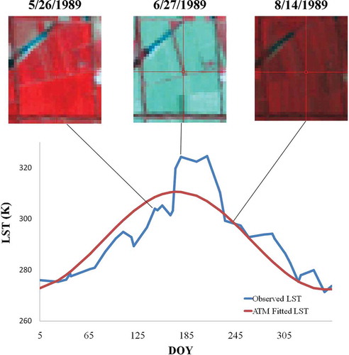
The average RMSE was 4.8%, 4.4%, and 3.8% for the 1990, 2001, and 2014 periods, respectively. Similar to the high MAST SD, RMSE of farmland was higher than that of urban areas (Figure 9). This result was not consistent with a previous study demonstrating that vegetated areas had a lower RMSE than urban areas (Bechtel 2015); and this was because the seasonal changes in the cultivation system. In the study area, winter wheat was sown in late October and harvested in early June of the following year; and after that, summer crops (such as summer maize) were sown. As a result, the vegetation fraction during late June and late July was low, which led to a high LST for these months and produced the relatively large RMSE in the ATM model results. In addition, the high LST in June and July may have caused MAST overestimation for cropland (Figure 10).

Figure 9. RMSE of the ATM model during the three periods.

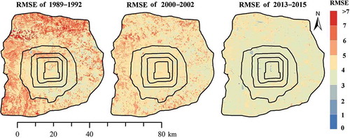
Figure 10. The cropland and the LST cycle of cropland in 1989. The color images are false color.

4.3. Spatial and temporal characteristics of %ISA variation

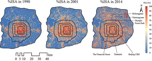
The mean %ISA in 1990, 2001, and 2014 was approximately 16.74%, 25.72%, and 36.31%, respectively. To quantify the trend of urban expansion, we divided %ISA into three levels of urban land: high (%ISA > 70%), moderate (30% < %ISA < 70%), and low density (%ISA <30%) (Table 2).

Table 2. Changes in urban land cover categories in Beijing from 1992 to 2014 (km²).

		Low-density urban land	Moderate-density urban land	High-density urban land
1990	Inside third ring	21.25	39.31	97.77
	Between third and fifth ring	270.57	123.43	114.66
	Between fifth and sixth ring	1383.10	165.31	68.42
2001	Inside third ring	21.13	46.58	90.62
	Between third and fifth ring	155.81	185.99	166.87
	Between fifth and sixth ring	1155.39	351.37	110.07
2014	Inside third ring	20.96	55.14	82.23
	Between third and fifth ring	143.62	173.47	191.58
	Between fifth and sixth ring	895.04	400.24	321.56

Figure 11 illustrates that in 1990 high-density urban land was mainly located within the fourth ring road. In addition, there were other significantly built-up areas within the residential regions of Tongzhou District and Shijingshan District, located beyond the west and east fifth ring road. Low-density urban areas such as mountainous and crop-covered land were located in rural areas outside the fifth ring road. Within the third ring road, high- and moderate-density urban land areas (mainly industrial and residential land) covered 97.77 and 39.31 km², which accounted for 61.75% and 24.83% of the total area within the third ring road, respectively. However, the low-density urban areas (mainly cropland and forests in mountainous areas) covered 270.57 km² between the third and fifth ring roads, and 1383.1 km² between the fifth and sixth ring roads, accounting for 53.19% and 85.54% of the areas in the corresponding belts. The high-density urban land outside the fifth ring road consisted of small villages and towns in rural areas covering 68.42 km².

Figure 11. %ISA maps for the years of 1990, 2001, and 2014.

From 1990 to 2001, Beijing experienced intra-urban land transformation and outward urban expansion (Figure 11). In the central urban area (within the third ring), high-density urban areas decreased by 7.15 km², moderate-density areas increased, and low-density urban areas experienced no significant change. These results are consistent with observations of increased vegetation in the central urban area of Beijing over the same time period (Jun and Zhou 2007). Several factors contributed to the increase in moderate-density urban areas. Single-story houses with a low greening rate (average of 9.3%) were abundant in residential areas in the early 1990s. In the early 2000s, some traditional residential areas were replaced by residential communities with improved greening (average greening of 28.3%) (Han et al. 1998). New infrastructure with additional green space was also constructed in inner-city areas to improve the urban environment (Dai, Ma, and Chen 2005; Kuang 2012). In addition, some residential areas with high urban density levels were converted to business districts with relatively higher greening rates, such as the Beijing Central Business District between the east third and fourth ring roads and Beijing Financial Street inside the west second ring road. In contrast, the urban expansion centered around the original city and extended to the fifth ring road, as well as the residential areas in Tongzhou District and Shijingshan District (Jiang et al. 2007; Dai, Ma, and Chen 2005). Areas of high and moderate urban density increased by 62.56 and 52.21 km², between the third and fifth ring roads, and by 41.65 and 186.06 km², between the fifth and sixth ring roads, respectively. Increases in high- and moderate-density urban areas occurred mainly in residential regions such as Huilongguan and Tiantongyuan, where the area of cropland (low construction density) subsequently decreased.

From 2001 to 2014, residential communities continued to replace traditional residential areas in the urban center, which led to a decrease in high-density urban areas and an increase in moderate-density construction areas, such as Tiantanlu within the second ring road. Thus, the most significant change outside the fifth ring road was the increment of high-density urban areas, which increased by more than 210 km² during this period. The residential areas continued to expand; for example, in the north, the floor area of Huilongguan increased from 0.8 km² to 8.6 km² between 2001 and 2014 (Li, Feng et al. 2013). In addition, satellite towns outside the fifth ring road expanded significantly, and a “multi-nuclei” development strategy was developed to assign different urban functions to different function zones (Kuang 2012). The rapid expansion of built-up areas was consistent with the fact that more than half of the city population residing outside the fifth ring road in 2014 (Beijing Statistics Bureau 2015).

4.4. Spatial and temporal characteristics of RMAST variation

The average RMAST in 1989–1992, 2000–2002, and 2013–2015 was 2.32, 3.23, and 3.62 K, respectively (Figure 12). In 1990, RMAST was relatively high in the urban center, particularly within the south second ring road where the MAST was 4 K higher than the reference area. Moreover, there were some hotspots in an area of barren land outside the fifth ring road, which contributed to the high RMAST. The mountain and farmland areas showed relatively low RMAST (RMAST < 2 K), although the RMAST of farmland areas was nearly 2 K higher than that of mountainous areas.

Figure 12. RMAST maps for the three periods of 1989–1992, 2000–2002, and 2013–2015.

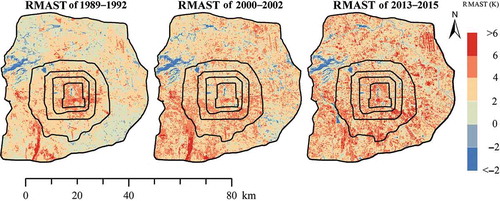
In general, the RMAST of the study area increased between the 1989–1992 and 2000–2002 periods. Within the urban center, although %ISA decreased in some residential areas, MAST did not experience a significant decline. In residential areas where %ISA remained relatively high (>90%), such as in Tiantanlu, RMAST increased to more than 7 K. Between the third and sixth ring roads, the airport had a high RMAST (>4 K), and newly constructed residential areas between the fourth and fifth ring roads showed an increasing prevalence of hotspots.

In 2014, areas of high RMAST (>4 K) were mainly distributed within the second ring road, between the south fourth and sixth ring roads and outside the northeast fifth ring road. The area around the north fifth ring road where the Olympic Forest Park was constructed in 2007 showed the greatest decline in MAST, with the RMAST below 2 K. Mountainous areas in the northwest still had relatively low LST (lower than 290 K), but the areas with low RMAST decreased relative to 2001.

4.5. Relationship between %ISA and RMAST

To determine the relationship between %ISA and RMAST, we randomly selected 5000 points using Hawth’s Tools (Hawthorne 2015), removing sample points located within waterbodies. A zonal analysis was then applied to evaluate the mean LST for each 1% increment of %ISA from 0% to 100% for each period (1989–1992, 2000–2002, and 2013–2015). Similar to previous studies, the mean RMAST showed significant positive correlation to mean %ISA (R² > 0.9) in all three periods (Figure 13), which indicated that RMAST increased with %ISA generally. For example, in all timeframes, the airport in the northeast section of the city with %ISA >95% had a high RMAST, while the mountainous area in the northwest section of the city remained cool (Yuan and Bauer 2007). In addition, the RMAST for each increment of %ISA varied significantly, the SD of each MAST exceeded 1 K, and the SD of RMAST in areas with low %ISA was higher than in areas with high %ISA.

Figure 13. Zonal analysis of correlation between mean RMAST and mean %ISA.

Notes: For the RMAST in this figure, 1990, 2000, and 2014 were corresponding to 1989–1992, 2000–2002, and 2013–2015 time periods, respectively.

Several factors may have contributed to the variation in RMAST. First, different land use in areas with similar %ISA could lead to variations in the RMAST. For example, land use types with low %ISA were forests, farmland, and bare soil, and the RMAST of farmland was 2 K higher than of forests (see Section 3.4) and the RMAST of bare soil was higher than that of forests or farmland. In addition, forests located on sunnier slopes had relatively higher RMAST than those located on shaded slopes. Moreover, Li et al. (2011) found that industrial land had higher LST than residential areas with similar %ISA. In another study, Li et al. (2014) showed that the LST of industrial areas and institutional areas was similar, although the vegetation fraction differed. Thus, different land use could lead to variations in RMAST for areas with similar %ISA, particularly in areas with low %ISA. A second factor is the strong influence of building morphology on RMAST. For example, Li et al. (2011) found that high-rise residential areas have much lower LST than low-rise residential areas, although the buildings in both areas are considered residential. Third, the spatial distribution of land cover could also lead to variations in RMAST for the same %ISA. For pixels with high %ISA values, those with low RMAST were located adjacent to farmland, and those with high RMAST were primarily in the urban center. For pixels with low %ISA, RMAST was relatively higher in the forests of an urban park than in mountainous areas. Moreover, the spatial parameters of land cover patterns, such as total area and shape index, could also contribute to variations in the LST (Rhee, Park, and Lu 2014).

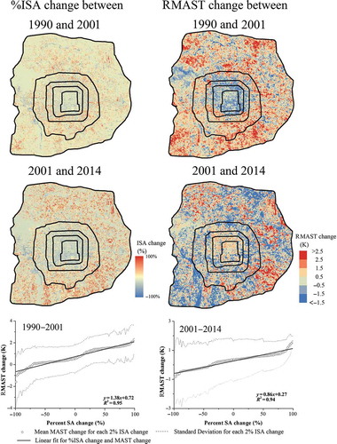
Change detection was used to derive temporal difference maps between %ISA and RMAST to determine the relationship between changes in %ISA and MAST. In addition, zonal analysis was employed to evaluate the change in mean RMAST for each 2% increment of %ISA change from −100% to 100% (Figure 14). Changes in RMAST increased with changes in %ISA. For example, %ISA increased by more than 50% between the third and fifth ring roads because most farmland in rural areas was converted to built-up areas between 1990 and 2001, while RMAST rose by more than 1.5 K in the corresponding areas. However, RMAST did not change significantly within the third ring road where %ISA decreased. Moreover, in areas where %ISA remained unchanged, RMAST increased by 0.7 K between 1990 and 2001 and by 0.3 K between 2001 and 2014. To further analyze these areas, we defined a change in %ISA between −5% and 5% to be areas where %ISA did not change. Table 3 shows that the majority of the areas where %ISA did not change had high %ISA (%ISA > 60%). Thus, an increase in RMAST in these areas may be due to an increase in anthropogenic heat flux. The average population density of suburban areas (Chaoyang, Fengtai, Haidian, and Shijingshan Districts) increased from 3101 to 5007 people/km² between 1990 and 2001, and increased to 7488 people/km² in 2010. The electric power consumption of residents also increased from 297 million kWh to 1003 million kWh between 1990 and 2001, and increased to 2230 million kWh in 2013. Moreover, the average energy consumption increased from 408.2 kg to 684.3 kg between 2000 and 2012 (as kg of coal equivalent) (Beijing Statistics Bureau 2014). Therefore, human metabolism and heat flux released by electrical consumption (e.g., lighting, heating, and air conditioning) and fuel burning (e.g., automobiles) contributed to an increase in anthropogenic heat.

Table 3. Distribution of pixels where %ISA change is between −5% and 5%.

	Proportion of pixels in each 10% %ISA interval (%)
%ISA	Between 2001 and 1990	Between 2014 and 2001
0–10	6.99	8.01
10–20	6.33	6.97
20–30	6.31	6.42
30–40	6.66	6.78
40–50	7.44	7.68
50–60	8.82	9.22
60–70	10.71	11.01
70–80	13.07	12.38
80–90	14.49	12.88
90–100	19.18	18.65

Notes: In this table, we used all pixels in our study area rather than the randomly selected 5000 points. First, we assumed that %ISA changes from −5% to 5% were areas of no change. Then, we divided the pixels within this range into 10 intervals based on their original %ISA value. For example, there were 251,306 pixels where the %ISA change was between −5% and 5% from 1990 to 2001, and among these pixels, the %ISA values of 17,557 pixels were between 0% and 10% in 1990. Thus, the proportion of pixels in the 0–10% %ISA interval between 1990 and 2001 was 6.99%.

Figure 14. %ISA and RMAST change maps derived by the image difference method.

Notes: For the RMAST in this figure, 1990, 2000, and 2014 were corresponding to 1989–1992, 2000–2002, and 2013–2015 time periods, respectively.

5. Conclusions and limitations

In this study, we used Landsat TM, ETM+, and OLI images that provided coverage up to the sixth ring road of Beijing to analyze changes in %ISA and RMAST between 1990 and 2014. The main conclusions are as follows:

1. From 1990 to 2001, Beijing exhibited internal urban land transformation and outward urban expansion. In the urban center (within the third ring road), high-density urban areas decreased by almost 7 km² and moderate-density urban areas increased, with both moderate- and high-density urban areas increasing significantly outside the third ring road.

2. From 2001 to 2014, a new urban planning design for “multi-nuclei” development resulted in the rapid expansion of both central urban and satellite towns outside the fifth ring road, where moderate- and high-density urban areas increased by 30 and 210 km², respectively.

3. RMAST generally increased with %ISA. During 1990–2001 and 2001–2014, RMAST increased by more than 1.5 K, mainly between the south third and sixth ring roads, and outside the fifth ring road where %ISA increased by more than 50%. RMAST also varied significantly for the same %ISA, which may be attributable to different land use types, building morphology, and the spatial distribution of buildings and vegetation. The average RMAST increased by 0.7 K between 1990 and 2001 and by 0.3 K between 2001 and 2014, while the %ISA did not change. Increasing anthropogenic heat generated by a growing population may have contributed to the increase in average RMAST.

At the medium spatial resolution of the Landsat data, the use of %ISA at the sub-pixel level described the urban components more continuously compared to the LULC classification method. In addition, the MAST extracted from an ATM used the annual LST cycle to describe the LST distribution, and the MAST from the model was comparable when analyzing multiyear changes in LST. To reduce the systematic error in applying NSMA to extract %ISA, the study area was divided into three levels using 30% and 70% of %ISA as thresholds. Three land use categories of low, moderate, and high %ISA were used to analyze urban expansion. In addition, we used the blackbody temperature to drive the ATM and extract MAST with ε = 1, which may underestimate the LST, especially in built-up areas where ε is lower than in forests and cropland with high vegetation fraction. Therefore, the MAST variation between urban and vegetated areas may be slightly underestimated in this study.

Recently, new satellites such as SPOT-6 and Gao Fen have been launched to improve observations of the land surface. In the future, we will continue to monitor urban expansion and changes in LST using images from new satellites to provide reliable information for urban planning decisions.

Disclosure statement

No potential conflict of interest was reported by the authors.

Additional information

Funding

This work was supported by the National Natural Science Foundation of China [grant number 41371416], [grant number 41371358]; Science and Technology Plan of Yunnan Province, China [grant number 2010AD004].

Appendix

Table A1. Landsat images used in this study.

	Landsat image between 1989 and 1992	Landsat image between 2000 and 2002	Landsat image between 2013 and 2015
Landsat 4	1989042
Landsat 5	1989066 1989098 1989146 1989178 1989210 1989226 2989290 1989306 1989322 1989336 1989354 1990005 1990037 1990085 1990117 1990149 1990165 1990197 1990261 1990293 1990325 1990341 1991072 1991088 1991120 1991136 1991168 1991171 1991232 1991251 1991280 1991312 1991363 1992027 1992043 1992107 1992155	2000033 2000081 2000097 2000129 2000145 2000161 2000257 2000289 2000305 2000353 2001103 2001083 2001131 2001147 2001195 2001227 2001243 2001323 2001355 2002070 2002198 2002278
Landsat 7		2000121 2000137 2000169 2000233 2000345 2001043 2001091 2001107 2001139 2001155 2001187 2001219 2001267 2001315 2001331 2001363 2002030 2002046 2002078 2002142 2002158 2002190 2002222 2002286 2002318 2002334	2013044 2013060 2013076 2013092 2013108 2013124 2013140 2013204 2013268 2013284 2013300 2013316 2013332 2013348 2013364 2014015 2014063 2014079 2014095 2014127 2014159 2014191 2014207 2014223 2014239 2014287 2014335 2014351 2015002 2015034 2015066 2015082 2015114 2015146
Landsat 8			2013132 2013164 2013212 2013244 2013276 2013308 2013324 2013340 2013356 2014103 2014119 2014135 2014231 2014247 2014263 2014279 2014359 2015010 2015074 2015106 2015122 2015138

Note: The numbers listed in the table are the year and day of year (DOY) for each Landsat image.

References

- Amiri, R., Q. H. Weng, A. Alimohammadi, and S. K. Alavipanah. 2009. “Spatial-Temporal Dynamics of Land Surface Temperature in Relation to Fractional Vegetation Cover and Land Use/Cover in the Tabriz Urban Area, Iran.” Remote Sensing of Environment 113 (12): 2606–2617. doi:10.1016/j.rse.2009.07.021.
- Bechtel, B. 2012. “Robustness of Annual Cycle Parameters to Characterize the Urban Thermal Landscapes.” IEEE Geoscience and Remote Sensing Letters 9 (5): 876–880. doi:10.1109/lgrs.2012.2185034.
- Bechtel, B. 2015. “A New Global Climatology of Annual Land Surface Temperature.” Remote Sensing 7 (3): 2850–2870. doi:10.3390/rs70302850.
- Beijing Statistics Bureau. 2012. Beijing Statistical Yearbook of 2012. China Statistics Press. http://www.bjstats.gov.cn/nj/main/2012-tjnj/index.htm.
- Beijing Statistics Bureau. 2014. Beijing Statistical Yearbook of 2014. China Statistics Press. http://www.bjstats.gov.cn/nj/main/2014-tjnj/CH/index.htm.
- Beijing Statistics Bureau. 2015. “Population Situation of Beijing in 2014.” Beijing Statistics Bureau China. Accessed 13 April 2015. http://www.bjstats.gov.cn/rkjd/sdjd/201506/t20150624_294864.htm
- Cai, G. Y., M. Y. Du, and Y. Xue. 2011. “Monitoring of Urban Heat Island Effect in Beijing Combining ASTER and TM Data.” International Journal of Remote Sensing 32 (5): 1213–1232. doi:10.1080/01431160903469079.
- Cao, X., A. Onishi, J. Chen, and H. Imura. 2010. “Quantifying the Cool Island Intensity of Urban Parks Using ASTER and IKONOS Data.” Landscape and Urban Planning 96 (4): 224–231. doi:10.1016/j.landurbplan.2010.03.008.
- Chander, G., B. L. Markham, and D. L. Helder. 2009. “Summary of Current Radiometric Calibration Coefficients for Landsat MSS, TM, ETM+, and EO-1 ALI Sensors.” Remote Sensing of Environment 113 (5): 893–903. doi:10.1016/j.rse.2009.01.007.
- Chen, X.-L., H.-M. Zhao, P.-X. Li, and Z.-Y. Yin. 2006. “Remote Sensing Image-Based Analysis of the Relationship between Urban Heat Island and Land Use/Cover Changes.” Remote Sensing of Environment 104 (2): 133–146. doi:10.1016/j.rse.2005.11.016.
- Dai, Q., J. W. Ma, and X. Chen. 2005. “Research on the Land Use Change with Beijing Ring Road Driven Using Remote Sensing Change Detection.” Journal of Remote Sensing 9 (3): 314–322.
- Ding, H. Y., and W. Z. Shi. 2013. “Land-Use/Land-Cover Change and Its Influence on Surface Temperature: A Case Study in Beijing City.” International Journal of Remote Sensing 34 (15): 5503–5517. doi:10.1080/01431161.2013.792966.
- Gaffin, S. R., C. Rosenzweig, R. Khanbilvardi, L. Parshall, S. Mahani, H. Glickman, R. Goldberg, R. Blake, R. B. Slosberg, and D. Hillel. 2008. “Variations in New York City’s Urban Heat Island Strength over Time and Space.” Theoretical and Applied Climatology 94 (1–2): 1–11. doi:10.1007/s00704-007-0368-3.
- Gottsche, F.-M., and F. S. Olesen. 2001. “Modelling of Diurnal Cycles of Brightness Temperature Extracted from METEOSAT Data.” Remote Sensing of Environment 76 (3): 337–348. doi:10.1016/s0034-4257(00)00214-5.
- Han, L. L., R. Z. Gu, X. X. Zhang, and H. Li. 1998. “Current Situation and Problem of Residential Area Green in Beijing.” Beijing Landscape 18 (2): 17–23.
- Hawthorne, B. 2015. “Hawth’s analysis tools for ArcGIS1.” Accessed 30 January. http://www.spatialecology.com/htools/overview.php
- IPCC. 2014. “Climate Change 2014 Synthesis Report.” Accessed 15 July 2015. http://www.ipcc.ch/report/ar5/syr/
- Jiang, F., S. H. Liu, H. Yuan, and Q. Zhang. 2007. “Measuring Urban Sprawl in Beijing with Geo-Spatial Indices.” Journal of Geographical Sciences 17 (4): 469–478. doi:10.1007/s11442-007-0469-z.
- Jimenez-Munoz, J. C., J. Cristobal, J. A. Sobrino, G. Soria, M. Ninyerola, and X. Pons. 2009. “Revision of the Single-Channel Algorithm for Land Surface Temperature Retrieval from Landsat Thermal-Infrared Data.” IEEE Transactions on Geoscience and Remote Sensing 47 (1): 339–349. doi:10.1109/tgrs.2008.2007125.
- Jun, Y., and J. X. Zhou. 2007. “The Failure and Success of Greenbelt Program in Beijing.” Urban Forestry & Urban Greening 6 (4): 287–296. doi:10.1016/j.ufug.2007.02.001.
- Kaufmann, R. K., K. C. Seto, A. Schneider, Z. T. Liu, L. M. Zhou, and W. L. Wang. 2007. “Climate Response to Rapid Urban Growth: Evidence of a Human-Induced Precipitation Deficit.” Journal of Climate 20 (10): 2299–2306. doi:10.1175/jcli4109.1.
- Kuang, W. H. 2012. “Spatio-Temporal Patterns of Intra-Urban Land Use Change in Beijing, China between 1984 and 2008.” Chinese Geographical Science 22 (2): 210–220. doi:10.1007/s11769-012-0529-x.
- Li, F. R., J. Feng, J. Liu, and Z. L. Li. 2013. “The Life Time and Space Reconfiguration of Residents in Large Communities in the Context of Suburbanization: A Case Study of Huilongguan.” Human Geography 28 (3): 27–33, 113.
- Li, G. Y., D. S. Lu, E. Moran, and S. Hetrick. 2013. “Mapping Impervious Surface Area in the Brazilian Amazon Using Landsat Imagery.” Giscience & Remote Sensing 50 (2): 172–183. doi:10.1080/15481603.2013.780452.
- Li, J. X., C. H. Song, L. Cao, F. G. Zhu, X. L. Meng, and J. G. Wu. 2011. “Impacts of Landscape Structure on Surface Urban Heat Islands: A Case Study of Shanghai, China.” Remote Sensing of Environment 115 (12): 3249–3263. doi:10.1016/j.rse.2011.07.008.
- Li, W. F., Y. Bai, Q. W. Chen, K. He, X. H. Ji, and C. M. Han. 2014. “Discrepant Impacts of Land Use and Land Cover on Urban Heat Islands: A Case Study of Shanghai, China.” Ecological Indicators 47: 171–178. doi:10.1016/j.ecolind.2014.08.015.
- Li, Y.-Y., H. Zhang, and W. Kainz. 2012. “Monitoring Patterns of Urban Heat Islands of the Fast-Growing Shanghai Metropolis, China: Using Time-Series of Landsat TM/ETM+ Data.” International Journal of Applied Earth Observation and Geoinformation 19: 127–138. doi:10.1016/j.jag.2012.05.001.
- Li, Z.-L., B.-H. Tang, H. Wu, H. Z. Ren, G. Yan, Z. Wan, I. F. Trigo, and J. A. Sobrino. 2013. “Satellite-Derived Land Surface Temperature: Current Status and Perspectives.” Remote Sensing of Environment 131: 14–37. doi:10.1016/j.rse.2012.12.008.
- Liu, H., and Q. H. Weng. 2009. “Scaling Effect on the Relationship between Landscape Pattern and Land Surface Temperature: A Case Study of Indianapolis, United States.” Photogrammetric Engineering & Remote Sensing 75 (3): 291–304. doi:10.14358/PERS.75.3.291.
- McFeeters, S. K. 1996. “The Use of the Normalized Difference Water Index (NDWI) in the Delineation of Open Water Features.” International Journal of Remote Sensing 17 (7): 1425–1432. doi:10.1080/01431169608948714.
- Phinn, S., M. Stanford, P. Scarth, A. T. Murray, and P. T. Shyy. 2002. “Monitoring the Composition of Urban Environments Based on the Vegetation-Impervious Surface-Soil (VIS) Model by Subpixel Analysis Techniques.” International Journal of Remote Sensing 23 (20): 4131–4153. doi:10.1080/01431160110114998.
- Powell, S. L., W. B. Cohen, Z. Q. Yang, J. D. Pierce, and M. Alberti. 2008. “Quantification of Impervious Surface in the Snohomish Water Resources Inventory Area of Western Washington from 1972–2006.” Remote Sensing of Environment 112 (4): 1895–1908. doi:10.1016/j.rse.2007.09.010.
- Rhee, J. Y., S. Park, and Z. Y. Lu. 2014. “Relationship between Land Cover Patterns and Surface Temperature in Urban Areas.” GIScience & Remote Sensing 51 (5): 521–536. doi:10.1080/15481603.2014.964455.
- Ridd, M. K. 1995. “Exploring a V-I-S (Vegetation-Impervious Surface-Soil) Model for Urban Ecosystem Analysis through Remote-Sensing – Comparative Anatomy for Cities.” International Journal of Remote Sensing 16 (12): 2165–2185. doi:10.1080/01431169508954549.
- Rizwan, A. M., L. Y. C. Dennis, and C. B. Liu. 2008. “A Review on the Generation, Determination and Mitigation of Urban Heat Island.” Journal of Environmental Sciences-China 20 (1): 120–128. doi:10.1016/s1001-0742(08)60019-4.
- Sexton, J. O., D. L. Urban, M. J. Donohue, and C. H. Song. 2013. “Long-Term Land Cover Dynamics by Multi-Temporal Classification across the Landsat-5 Record.” Remote Sensing of Environment 128: 246–258. doi:10.1016/j.rse.2012.10.010.
- Shepherd, J. M., and S. J. Burian. 2003. “Detection of Urban-Induced Rainfall Anomalies in a Major Coastal City.” Earth Interactions 7 (4): 1–17. doi:10.1175/1087-3562(2003)007<0001:DOUIRA>2.0.CO;2.
- Streutker, D. R. 2002. “A Remote Sensing Study of the Urban Heat Island of Houston, Texas.” International Journal of Remote Sensing 23 (13): 2595–2608. doi:10.1080/01431160110115023.
- Sun, R. H., A. L. Chen, L. D. Chen, and Y. H. Lu. 2012. “Cooling Effects of Wetlands in an Urban Region: The Case of Beijing.” Ecological Indicators 20: 57–64. doi:10.1016/j.ecolind.2012.02.006.
- Tang, Q., L. Wang, B. Li, and J. Yu. 2012. “Towards a Comprehensive Evaluation of V-I-S Sub-Pixel Fractions and Land Surface Temperature for Urban Land-Use Classification in the USA.” International Journal of Remote Sensing 33 (19): 5996–6019. doi:10.1080/01431161.2012.675453.
- Torbick, N., and M. Corbiere. 2015. “Mapping Urban Sprawl and Impervious Surfaces in the Northeast United States for the past Four Decades.” GIScience & Remote Sensing 1–19. doi:10.1080/15481603.2015.1076561.
- University of Wyoming. 2015. “Upperair air data.” Accessed 26 June. http://weather.uwyo.edu/upperair/seasia.html
- USGS. 2015. “USGS-earthexplorer.” Accessed 26 June. http://earthexplorer.usgs.gov/
- Weng, Q. H. 2009. “Thermal Infrared Remote Sensing for Urban Climate and Environmental Studies: Methods, Applications, and Trends.” ISPRS Journal of Photogrammetry and Remote Sensing 64 (4): 335–344. doi:10.1016/j.isprsjprs.2009.03.007.
- Weng, Q. H. 2012. “Remote Sensing of Impervious Surfaces in the Urban Areas: Requirements, Methods, and Trends.” Remote Sensing of Environment 117: 34–49. doi:10.1016/j.rse.2011.02.030.
- Weng, Q. H., and P. Fu. 2014. “Modeling Annual Parameters of Clear-Sky Land Surface Temperature Variations and Evaluating the Impact of Cloud Cover Using Time Series of Landsat TIR Data.” Remote Sensing of Environment 140: 267–278. doi:10.1016/j.rse.2013.09.002.
- Weng, Q. H., and D. S. Lu. 2008. “A Sub-Pixel Analysis of Urbanization Effect on Land Surface Temperature and Its Interplay with Impervious Surface and Vegetation Coverage in Indianapolis, United States.” International Journal of Applied Earth Observation and Geoinformation 10 (1): 68–83. doi:10.1016/j.jag.2007.05.002.
- Weng, Q. H., and D. S. Lu. 2009. “Landscape as a Continuum: An Examination of the Urban Landscape Structures and Dynamics of Indianapolis City, 1991–2000, by Using Satellite Images.” International Journal of Remote Sensing 30 (10): 2547–2577. doi:10.1080/01431160802552777.
- Wong, K. V., A. Paddon, and A. Jimenez. 2013. “Review of World Urban Heat Islands: Many Linked to Increased Mortality.” Journal of Energy Resources Technology 135 (2): 022101–022112. doi:10.1115/1.4023176.
- Wu, C. S. 2004. “Normalized Spectral Mixture Analysis for Monitoring Urban Composition Using ETM Plus Imagery.” Remote Sensing of Environment 93 (4): 480–492. doi:10.1016/j.rse.2004.08.003.
- Wu, C. S., and A. T. Murray. 2003. “Estimating Impervious Surface Distribution by Spectral Mixture Analysis.” Remote Sensing of Environment 84 (4): 493–505. doi:10.1016/s0034-4257(02)00136-0.
- Xu, H. Q., D. F. Lin, and F. Tang. 2013. “The Impact of Impervious Surface Development on Land Surface Temperature in a Subtropical City: Xiamen, China.” International Journal of Climatology 33 (8): 1873–1883. doi:10.1002/joc.3554.
- Yang, P., G. Y. Ren, and W. D. Liu. 2013. “Spatial and Temporal Characteristics of Beijing Urban Heat Island Intensity.” Journal of Applied Meteorology and Climatology 52 (8): 1803–1816. doi:10.1175/jamc-d-12-0125.1.
- Yuan, F., and M. E. Bauer. 2007. “Comparison of Impervious Surface Area and Normalized Difference Vegetation Index as Indicators of Surface Urban Heat Island Effects in Landsat Imagery.” Remote Sensing of Environment 106 (3): 375–386. doi:10.1016/j.rse.2006.09.003.
- Zhang, C., Y. L. Chen, and D. S. Lu. 2015. “Detecting Fractional Land-Cover Change in Arid and Semiarid Urban Landscapes with Multitemporal Landsat Thematic Mapper Imagery.” Giscience & Remote Sensing 1–23. doi:10.1080/15481603.2015.1071965.
- Zhang, X., T. Zhong, K. Wang, and Z. Cheng. 2009. “Scaling of Impervious Surface Area and Vegetation as Indicators to Urban Land Surface Temperature Using Satellite Data.” International Journal of Remote Sensing 30 (4): 841–859. doi:10.1080/01431160802395219.
- Zhang, Y. S., I. O. A. Odeh, and C. F. Han. 2009. “Bi-Temporal Characterization of Land Surface Temperature in Relation to Impervious Surface Area, NDVI and NDBI, Using a Sub-Pixel Image Analysis.” International Journal of Applied Earth Observation and Geoinformation 11 (4): 256–264. doi:10.1016/j.jag.2009.03.001.
- Zhu, Z., and C. E. Woodcock. 2012. “Object-Based Cloud and Cloud Shadow Detection in Landsat Imagery.” Remote Sensing of Environment 118: 83–94. doi:10.1016/j.rse.2011.10.028.