A support vector machine classifier based on a new kernel function model for hyperspectral data

Abstract

The kernel function is a key factor to determine the performance of a support vector machine (SVM) classifier. Choosing and constructing appropriate kernel function models has been a hot topic in SVM studies. But so far, its implementation can only rely on the experience and the specific sample characteristics without a unified pattern. Thus, this article explored the related theories and research findings of kernel functions, analyzed the classification characteristics of EO-1 Hyperion hyperspectral imagery, and combined a polynomial kernel function with a radial basis kernel function to form a new kernel function model (PRBF). Then, a hyperspectral remote sensing imagery classifier was constructed based on the PRBF model, and a genetic algorithm (GA) was used to optimize the SVM parameters. On the basis of theoretical analysis, this article completed object classification experiments on the Hyperion hyperspectral imagery of experimental areas and verified the high classification accuracy of the model. The experimental results show that the effect of hyperspectral image classification based on this PRBF model is apparently better than the model established by a single global or local kernel function and thus can greatly improve the accuracy of object identification and classification. The highest overall classification accuracy and kappa coefficient reached 93.246% and 0.907, respectively, in all experiments.

Keywords:

• hyperspectral imagery
• classification
• support vector machine
• kernel function

1. Introduction

Hyperspectral remote sensing is a relatively new technology that is currently being investigated in many scientific fields. In comparison to classic multispectral sensors, hyperspectral sensors offer finer and more adjacent data composed of about 100–200 or more spectral bands with relatively narrow bandwidths (5–10 nm). These detailed spectral information makes it possible to discriminate different object types through their spectral response characteristics in various spectral bands (Linden and Hostert 2009; Pignatti et al. 2009; Hasanlou, Samadzadegan, and Homayouni 2015). However, due to the high-dimensional feature space and limited training samples of hyperspectral images, conventional statistical pattern identification methods have difficulty in classifying hyperspectral images (Plaza et al. 2009; Heiden et al. 2007; Chi, Feng, and Bruzzone 2008; Shao et al. 2014). Because it has a small training sample requirement and supports high-dimensional feature space, the support vector machine (SVM) method is significantly better than other machine learning methods (e.g., the artificial neutral network method) in small sample learning, noise reduction, learning efficiency, and so on (Guneralp, Filippi, and Hales 2013; Chen, Zhao, and Lin 2014; Lu et al. 2014). It can avoid the “curse of dimensionality” and over-learning problems and is very suitable for hyperspectral image classification (Foody and Mathur 2006; Mountrakis, Im, and Ogole 2011; Zhou, Lai, and Yu 2010; Sengur 2009; Kumar and Kar 2009).

The input data in the n-dimensional vector space are mapped into a high-dimensional feature space using kernel functions, in which a nonlinear problem in the input space is transformed into a linear problem in the feature space (Bai et al. 2008; Li, Im, and Beier 2013; Kim et al. 2014). The kernel function is a key factor to determine the performance of an SVM classifier and different types of kernel functions have a marked impact on classification results. Therefore, choosing and constructing appropriate kernel function models has been a hot topic in SVM studies (Jian and Zhao 2009). The complexity of the sample data distribution in high-dimensional feature space is mainly influenced by the kernel function: if the complexity is high, the obtained optimal separating hyperplane may be more complicated. When the separating hyperplane has less empirical risk, but its generalization ability (also called extrapolation ability or promotion ability) is weak, it will have serious over-learning issues; under opposite conditions, it will have under-learning issues. Kernel function selection has not formed a unified model and can only rely on the experience and the specific sample characteristics. This article summarized the kernel function theory and research findings and, based on this result, attempted to combine a polynomial kernel function with a radial basis kernel function to form a new kernel function model (PRBF) and constructed a hyperspectral remote sensing imagery classifier based on the PRBF model. Then, this article employed a genetic algorithm (GA) to optimize the SVM parameters to effectively avoid the blindness of artificial selection parameters and realize the automatic optimization of the SVM model and thus greatly improve the accuracy of object identification and classification.

2. Data and experimental area

2.1. Data characteristics

The Earth-Observing 1 (EO-1) satellite was launched from Vandenberg Air Force Base on 21 November 2000. This satellite was developed for the replacement of Landsat-7 and its equatorial crossing time is one minute behind Landsat-7. It has a sun-synchronous orbit with an altitude of 705 km, an inclination of 98.2 degrees and a period of 98.9 min (Goodenough et al. 2003; Wu 2001). The instrument payloads on the satellite are Hyperion, Advanced Land Imager (ALI) and Linear Etalon Imaging Spectrometer Array Atmospheric Corrector (LAC). Among them, Hyperion is a rare space-borne imaging spectrometer with a spectral region from 400 to 2500 nm that acquires data in push broom mode with two spectrometers: one visible and near infrared (VNIR) spectrometer (400–1000 nm) and one short-wave infrared (SWIR) spectrometer (90–2500 nm) (Moreira, Teixeira, and Galvao 2015). Each image of Hyperion has a 10-nm spectral resolution and a 30-m spatial resolution, but its swath width is only 7.7 km due to data storage and satellite transmission constraints. The data products are distributed in 242 bands (VNIR 1–70, SWIR 71–242). Due to the low signal for some channels and reducing the VNIR-SWIR overlap region, only 198 bands (VNIR 8–57, SWIR 77–224) are calibrated. The bands that are not calibrated are set to zero (Pignatti et al. 2009; Ungar et al. 2003).

Hyperion data are divided into L0 (Level 1) and L1 (Level 1): L0 is the raw datum and L1 is the user datum. L1 is divided into L1A (Level 1 Revision A), L1B (Level 1 Revision B), L1R (Level 1 Radiometrically Corrected) and L1Gst (Level 1 Geometric Systematic Terrain Corrected): L1A and L1B product data are initially generated by TRW, Inc.; L1R and L1Gst product data are generated later by the U.S. Geological Survey. L1R and L1Gst product data have been processed by spot removal, return wave correction, background removal, radiometric calibration, bad pixels repair and quality inspection. Therefore, L1R and L1Gst data are more often used.

2.2. Experimental area

In the Fujian Province of China, strongly undulating terrain and abnormal broken topography has caused the redistribution of zonal hydrothermal conditions in the Earth’s surface. This redistribution formed a complex and diverse ecological pattern. It highlights the remote sensing performance of capturing complex spatial variability and significant phase changes, which has always been challenging in remote sensing monitoring.

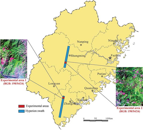
Taking into account the complexity of humid subtropical ecological patterns and the spatial applicability of this study in the Fujian Province, two locations were selected for the EO-1 Hyperion L1R hyperspectral remote sensing data (one located in the south subtropical coastal area, the other located in the middle subtropical inland area). Because the Hyperion hyperspectral image is only 7.7-km wide, it is difficult to determine the boundary of experimental areas using administrative divisions or ecological divisions, so this study chose a rectangular area in each image as the experimental area. The location map of these two experimental areas is shown in Figure 1.

Figure 1. The location map and Hyperion image of the experimental areas in the Fujian Province of China. For full colour versions of the figures in this article, please see the online version.

3. Methodology

3.1. SVM

The SVM method proposed by Vapnik et al. in the mid-1990s is a novel machine learning method based on Vapnik–Chervonenkis (VC) dimension theory and the structural risk minimization principle of statistical learning theory. The SVM method can achieve the best generalization ability by searching for a balance between model complexity and learning ability based on limited samples (Cortes and Vapnik 1995; Cristianini and Shawe-Taylor 2000; Rao et al. 2015). It aims to map the original data into a high-dimensional feature space through a nonlinear mapping function, where an optimal hyperplane that provides a maximum margin between the two classes is determined. The learning problems of SVM can be formulated as a convex quadratic programming problem to seek the global optimal solution. Therefore, it can avoid the problem of local extremes that exists in artificial neural networks and cleverly solve the dimension problem (Vapnik 2000).

SVM was originally developed from the optimal separating hyperplane in linearly separable case. An optimal separating hyperplane is able to not only correctly separate two classes with a 0 training error rate but also maximize the distance between the two classes (Jian and Zhao 2009; Xun and Wang 2015). An optimal separating hyperplane in two-dimensional case is shown in Figure 2, where triangle and square represent two class samples, H is the optimal separating line, H₁ and H₂ are two lines parallel to the optimal separating line and through the samples nearest the optimal separating line, the distance between H₁ and H₂ is the margin. The training sample points on H₁ and H₂ are called support vectors (SVs).

Figure 2. The schematic diagram of an optimal separating hyperplane.

Assume that a training dataset (x_i, y_i), i = 1,2,…,n, x_i∈R^d, y_i∈{+1,−1} is linearly separable, then a separating hyperplane can be expressed in the following form:

(1)

where ω is the weight vector of the separating hyperplane.

Determination of the optimal separating hyperplane needs to maximize , namely, minimize . Thus, solving the optimal separating hyperplane problem can be expressed as the following constrained optimization problem:

(2)

(3)

where Equation (2) is the objection function and Equation (3) is the constraint condition.

If the data are not linearly separable, they may be mapped into a high-dimensional feature space through a nonlinear mapping function, where they are linearly separable and an optimal separating hyperplane is determined. This nonlinear mapping can be achieved by defining an appropriate inner product function (Bai et al. 2008).

The optimal separating hyperplane function obtained after solving the above problem is given by

(4)

where K(x,x_i) is a kernel function that could be defined as the inner product of vectors x_i and x in the feature space, a_i* is the optimal solution, in which non-zero samples are the SVs, and b* is the classification threshold that may be obtained by any SV or any pair of SVs of the two classes.

When the two class training samples cannot be completely separated using the optimal separating hyperplane, we can introduce a slack factor ζ_i that allows misclassified samples to search for a balance between the generalization performance and the empirical risk (Zhang 2000). Thus, Equation (3) becomes as follows:

(5)

We also add a penalty term in the objective function and Equation (2) becomes

(6)

where C is a penalty parameter controlling the penalty for misclassified samples. The larger the C value, the higher the penalty for misclassified samples (Deng and Tian 2004; Scholkopf, Burges, and Smola 1998).

3.2. Kernel function

3.2.1. Kernel function’s implication

A kernel function is a nonlinear mapping function φ(·) to establish K(x, x_i) = φ(x)·φ(x_i). Random vector x in the n-dimensional vector space can be mapped into a high-dimensional feature space H by using kernel functions, i.e., φ: R^d→H, x→φ(x), where a linear separation is feasible (Bai et al. 2008). The schematic diagram of the SVM kernel function for the two-dimensional case is shown in Figure 3.

Figure 3. The schematic diagram of the SVM kernel function.

According to the theory of Hilbert-Schmidt, if a kernel function satisfies Mercer’s Theorem, it corresponds to the inner product in a mapping space. For any and , the sufficient and necessary condition is

(7)

In various practical applications of the kernel function, SVMs only store inner products in feature space, without having to know the specific form of the nonlinear mapping. The kernel function in the original input space essentially performs an implicit operation in the high-dimensional space after nonlinear function mapping.

3.2.2. Kernel function’s properties

1. Assume that K_l(x, x_i) and K₂(x, x_i) are kernel functions on X × X, the constant α ≥ 0, f(·) is a real-value function on X, φ: X→Rⁿ, K₃ is a kernel function on Rⁿ×Rⁿ, and B is a n × n symmetric positive semidefinite matrix; then, the following functions are still kernel functions (Shawe-Taylor and Cristianini 2004):

   ①K(x, x_i) = K_l(x, x_i) + K₂(x, x_i); ②K(x, x_i) = α K_l(x, x_i), ③K(x, x_i) = K_l(x, x_i) K₂(x, x_i), ④K(x, x_i) = f(x) f(x_i), ⑤K(x, x_i) = K₃(φ(x),φ(x_i)), ⑥K(x, x_i) = x^TB x_i.

2. Assume that K_l(x, x_i) is a kernel function on X × X and p(x) is a polynomial with a positive coefficient; then, the following functions are still kernel functions (Shawe-Taylor and Cristianini 2004):

   ①K(x, x_i) = p(K_l (x, x_i)), ②K(x, x_i) = exp(K_l (x, x_i)), ③K(x, x_i) = exp(−‖x-x_i‖²/2σ²).

As can be seen from the kernel function properties, if a kernel function satisfies Mercer’s Theorem, many new and more complex kernel functions based on the above operations could be constructed by the closure of addition and multiplication to meet the specific needs of each species (Wang 2006).

3.2.3. Common kernel function

Currently, kernel functions for SVMs can be divided into two categories: The first category is the global kernel function, and the second is the local kernel function. Global kernel functions, such as linear kernel, polynomial kernel and Sigmoid kernel functions, contain overall properties, i.e., data points far away from the test points in the dataset may also have an impact on the value of the kernel function. The generalization ability of global kernel functions is strong, but the learning ability is weak. Local kernel functions, such as radial basis kernel functions, are the ones with partial properties, i.e., only data points close to the test points in the dataset have an impact on the value of the kernel function. The generalization ability of local kernel functions is weak, but the learning ability is strong.

1. Linear kernel function (LKF)

A LKF, which is a global kernel function, can be formulated with the inner product of two vectors in linearly separable cases, as follows (Jian and Zhao 2009):

(8)

Using a linear kernel function, you can find a linear classifier with the best generalization in the original data space.

1. Polynomial kernel function (PKF)

A PKF is also a global kernel function, with a kernel form as follows (Jian and Zhao 2009):

(9)

where r is the offset coefficient (generally, its value is 1 according to experience) and d is the degree of the polynomial kernel. The larger the d value, the higher the mapping dimension (i.e., the optimal separating hyperplane structure is more complicated and its calculation is also larger). The VC dimension in the system can be controlled by selecting a different d value.

The overall properties of polynomial kernel functions (i.e., strong generalization ability and weak learning ability) may be weakened by increasing the d value. When r = 0 and d = 1, K(x, x_i) becomes a linear kernel function; thus, a linear kernel function can be regarded as a special case of polynomial kernel functions.

1. Sigmoid kernel function (SKF)

A SKF is also a global kernel function, using a hyperbolic tangent function (tanh) as follows (Bai et al. 2008):

(10)

where v is the scale parameter and w is the decay parameter. A sigmoid function is actually a multilayer perceptron neural network in which the node number and weight vectors of the hidden layer are determined automatically by algorithm in the training process, and then, the local minima problems that perplexed the neural network could not exist.

1. Radial basis kernel function (RBKF)

A RBKF is a local kernel function, and its kernel form is as follows (Bai et al. 2008):

(11)

where σ is the normalized parameter that determines kernel width around the center point and ‖x-x_i‖ is the norm of vector x-x_i that represents the distance between x and x_i.

RBKF is a strongly localized kernel function, and its learning ability is weakened with an increasing σ value. The smaller the σ value, the stronger the learning ability of SVMs (i.e., the empirical risk becomes smaller in the risk structure), but the SVM generalization ability is also worse, which makes the confidence interval larger. Therefore, to make the structural risk of the classifier as small as possible and increase its generalization ability, σ values should be properly selected.

3.3. PRBF kernel function

Global kernel functions and local kernel functions each have their own characteristics: the former have strong generalization ability and weak learning ability; the latter have weak generalization ability and strong learning ability. Among global kernel functions, PKF is the most widely used and most typical kernel function (Jian and Zhao 2009). Among local kernel functions, RBKF is the most widely used and most typical kernel function (Xun and Wang 2015; Rosa and Wiesmann 2013; Maxwell et al. 2014). Thus, in this study, to achieve an appropriate balance between the generalization ability and learning ability, PKF and RBKF were selected to constitute a new kernel function (polynomial and radial basis function, PRBF) model. Its expression is as follows:

(12)

where r is the offset coefficient (generally its value is 1 according to experience), d is the degree of the polynomial kernel, σ is the kernel width of RBF and e is the weight coefficient (0 ≤ e ≤ 1).

The weight coefficient e is used to balance the role of PKF with RBKF in PRBF. When e tends to zero, RBKF plays a dominant role in PRBF, whereas when e tends to 1, PKF plays a dominant role in PRBF. By adjusting the e value, PRBF can be adapted to different data distributions, which facilitates the introduction of auxiliary decisions based on a priori knowledge of a specific problem in the kernel function.

To compare the difference among PKF, RBKF and PRBF, the characteristic graph of each kernel function is shown in Figure 4, where x and x_i are one-dimensional vectors and the test input values x_i are 0.2.

Figure 4. Characteristic graphs of kernel functions: (a) PKF; (b) RBKF; (c) PRBF.

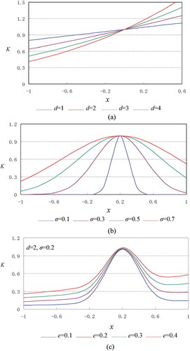
Figure 4(a) is a characteristic graph of PKF, where the polynomial degree (d) ​​was taken as 1, 2, 3, and 4, respectively. As can be seen from Figure 4(a):

1. Increasing the deviation between input data ​​x and test input value x_i, the K value is increased (decreased) on the right (left) side of x_i and is always greater than zero. Thus, it shows obvious overall properties (i.e., the data points far away from the test points in the dataset may also have an impact on the value of the kernel function).

2. The larger the d value, the larger the curvature of its curve and the distribution of the K value tends to be increasingly uneven. It is suggested that the overall properties of PKF will be weakened and its generalization ability (i.e., extrapolation ability) will become weaker with the increasing d value.

Figure 4(b) is a characteristic graph of RBKF, where the kernel width (σ) ​​was taken as 0.1, 0.3, 0.5, and 0.7, respectively, as shown in Figure 4(b):

1. The K value is larger in the vicinity of the test input value x_i. Increasing the deviation between ​​x and x_i decreases the K value. Thus, it shows obvious partial properties (i.e., only data points close to the test points in the dataset have an impact on the value of the kernel function).

2. The larger the σ value, the larger the curve control interval. The larger the σ value, the larger the K value corresponding to the same x and the more even its distribution tends to be. It is suggested that the partial properties of PBKF will be weakened and its learning ability will become weaker with an increasing σ value.

Figure 4(c) is a characteristic graph of PRBF, where the weight coefficient (e) ​​was taken as 0.1, 0.2, 0.3, and 0.4 and d ​​and σ were taken as 2 and 0.2. As shown in Figure 4(c), PRBF, which is an integrated global and local kernel function, has a greater impact on the data samples closer to the test points and also has a certain impact on the data samples far from the test points. It is suggested that PRBF is a strong kernel function model in both learning ability and generalization ability. Its learning ability is stronger than the global kernel function, and its generalization ability is stronger than the local kernel function.

3.4. Parameters optimization

In the PRBF-SVM classification model, the penalty parameter (C), polynomial degree (d), radial basis kernel width (σ) and weight coefficient (e) are four essential parameters that could directly affect the classification accuracy. This study adopted a two-step parameters optimization approach. We first used a GA to optimize the single kernel function (i.e., PKF and RBKF) parameters, respectively, to achieve optimal (i.e., the highest classification accuracy), and then used an adjustment method to optimize the weight coefficient (e), so as to determine the best combination of these two single kernel functions.

In the first step, GA was used to find the optimal values of PKF-SVM and RBKF-SVM parameters i.e. C, d, and σ. GA involves encoding mechanism, fitness function, genetic operators (including selection, crossover and mutation), operating parameters, and so on. Specifically, the processing was as follows: 1) randomly selecting an initial population composed with the parameters, normally encoded into binary format; 2) adopting a negative root mean square error (RMSE) as the fitness function to measure the pros and cons of the selected parameter value, and calculating the fitness of each individual in the population; 3) according to the fitness value, a roulette wheel selection method was used to select individuals into the next generation from the current population; 4) according to the crossover probability P_c, a single point crossover algorithm was used to form a new offspring; 5) according to the mutation probability P_m, the mutation operation was performed using a basic mutation algorithm, and a new individual was generated by randomly changing certain individual genes; 6) if the stopping condition is met, end the GA running and give the optimal solution for each parameter; otherwise, proceed with selection, crossover, mutation operation to generate new parameter values.

In the second step, we used an adjustment method to optimize the weight coefficient (e). The already-determined parameter values in the first step were substituted into PRBF kernel function. Next, consider which type of kernel function (PKF or RBKF) play a dominant in the mixed kernel function (PRBF), so that the PRBF-SVM has the optimal nonlinear processing ability. There are two ways to adjust parameter e: first, the program automatically searches operations with a step size set from on [0,1], which is more objective but runs longer for large datasets; second, some a priori knowledge is added to parameter adjustment, which is more subjective but often has good results. Of course, these two ways can be combined. For example, first using the latter to narrow the search range, and then using the former to search.

4. Experiment and analysis

4.1. Experiment 1

4.1.1. Hyperspectral data

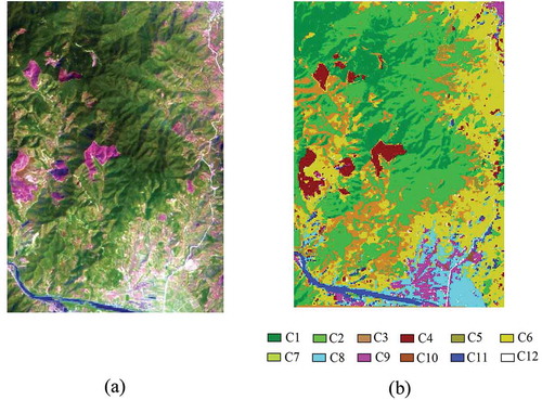
The experimental data preprocessed and fused before classification is the Hyperion hyperspectral imagery of experimental area 1 (see Section 2.2), and the image size is 450 × 660 pixels. We have reduced the number of bands to 157 (VNIR 8–57, SWIR 79–119, SWIR 134–164, SWIR 183–184, SWIR 188–220) by removing the bands covering the region of uncalibration, overlapping, small ground information and water absorption. Through field investigation and spectral analysis of the experimental area, ground object types were divided as follows: C1 (Chinese fir woodland), C2 (Masson pine woodland), C3 (shrub-grassland), C4 (burned area), C5 (orchard), C6 (tea plantation), C7 (dry land), C8 (economic crops), C9 (buildings), C10 (bare land), C11 (water) and C12 (road).

4.1.2. Training sample and test sample

The training sample sets for classification modeling and the test sample sets for classification accuracy were determined by referencing a 2.5-m spatial resolution SPOT5 satellite image and 1:10000 topographic maps (shown in Table 1). Then, the training samples were imported into the N-D Visualization module for rotating purification that was designed to remove impure pixels to improve the separability of different object training samples.

Table 1. Samples of different ground object types in experimental area 1.

Ground object type	C1	C2	C3	C4	C5	C6	C7	C8	C9	C10	C11	C12
Number of training samples	693	896	559	722	567	751	472	489	367	414	332	186
Number of test samples	724	884	651	706	613	768	422	469	326	439	283	156

4.1.3. GA optimization

We used a GA to optimize the three parameters (i.e., C, d and σ). The optimization intervals of each parameter were set as the following: C∈[0,1000], d∈[0,50], and σ∈[0.01,10]; the population size of GA was 50, crossover probability P_c was 0.8, mutation probability P_m was 0.25, evolutionary generation was 1000 and fitness function was a negative root mean square error (RMSE). Table 2 shows the highest classification accuracy achieved by the three kernel function models, respectively, in which the values of the kernel parameters and penalty parameters (C) were determined by automatic optimization methods.

Table 2. The comparison among the classification accuracies of different kernel functions in experimental area 1.

Kernel function	Kernel parameters	C	Overall classification accuracy (%)	Kappa coefficient	Classification time(s)
PKF	d = 3	100	86.172	0.824	8.15
RBKF	σ = 0.2	50	91.423	0.889	8.12
PRBF	σ = 0.2, d = 3, e = 0.3	80	93.246	0.907	8.28

As shown in Table 2, the classification accuracy of PKF-SVM was the lowest (i.e., the overall classification accuracy was 86.172% and the kappa coefficient was 0.824), and its classification time was 8.15 s; the classification accuracy of RBKF-SVM followed (i.e., the overall classification accuracy was 91.423% and the kappa coefficient was 0.889), and its classification time was 8.12 s; and the classification accuracy of PRBF-SVM was the highest (i.e., the overall classification accuracy was 93.246% and its kappa coefficient was 0.907), and its classification time was 8.28 s. Compared with PKF, the overall classification accuracy and kappa coefficient of PRBF-SVM were increased by 7.074% and 0.083, respectively. Compared with RBKF, the overall classification accuracy and kappa coefficient of PRBF-SVM were increased by 1.823% and 0.018, respectively. Thus, the SVM classifier based on PRBF achieved better classification results than a single PKF or RBKF with a similar classification time.

4.1.4. Adjustment of the weight coefficient

The weight coefficient (e) was used to balance the role of PKF with RBKF in the PRBF formula. In this study, we adopted an adjustment method to find the optimal e value. Table 3 shows the changes of the overall classification accuracy and kappa coefficients caused by different e values in experimental area 1.

Table 3. The classification accuracy of different weight coefficients in experimental area 1.

e	1–e	Overall classification accuracy (%)	Kappa coefficient
0.1	0.9	91.765	0.891
0.3	0.7	93.246	0.907
0.5	0.5	91.952	0.893
0.7	0.3	89.346	0.861
0.9	0.1	87.458	0.843

As shown in Table 3, with the increase in the e value​​, the overall classification accuracy of the model initially increased and then decreased following e = 0.3. In the first half of this process, the role of the first PKF was much weaker than RBKF (the ratio was 1:9); afterwards, the role of the former slightly enhanced and the latter role was slightly weakened until e = 0.3, when the highest classification accuracy was attained and the ratio became 3:7. In the last half of this process, the role of PFK continued to enhance as the role of RBKF continued to decline; the classification accuracy decreased until the ratio of the former to the latter became 9:1, when the classification accuracy was the lowest. Therefore, adjusting parameter e could control the balance of forces in regards to PKF and RBKF to make the model more responsive to the specific data distribution process (in this experimental data, the best classification results were attained at a ratio of 3:7).

4.1.5. Experimental results and analysis

Therefore, the results indicated that the SVM classification accuracy with the PRBF model consisting of PKF and RBKF was higher than an SVM classifier with a single kernel function model. In this experiment, the highest overall classification accuracy and kappa coefficient reached 93.246% and 0.907, respectively.

Figure 5(a) shows Hyperion hyperspectral image of experimental area 1. Figure 5(b) shows the SVM classification result based on optimized PRBF in experimental area 1, where σ, d, e, and C ​​were taken as 0.2, 3, 0.3, and 80, respectively. As seen from field investigation and land use maps, the classification accuracy rate of this classifier was very high for most objects. Its overall classification accuracy was 93.246%, and its kappa coefficient was 0.907. Moreover, the classification accuracies of some types of ground objects were also improved to varying degrees compared with PKF and RBKF, especially near the southern neighborhoods, where the question of poor partial classification accuracy caused by mixed multiple objects (such as road, bare land, buildings, dry land, etc.) had been alleviated.

Figure 5. (a) Hyperion hyperspectral image (RGB: 150/48/31) and (b) SVM classification image of the optimized PRBF in experimental area 1.

4.2. Experiment 2

Experiment 1 showed that the SVM classifier based on optimized PRBF was quite successful in the coastal areas of the Fujian Province. To further examine the performance of this classifier in the inland areas, we selected experimental area 2 located in the inland area of the Fujian Province to conduct the experimental work.

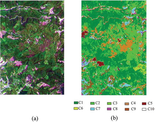
The experimental data preprocessed and fused before classification is the Hyperion hyperspectral imagery of experimental area 2 (see Section 2.2), and the image size is 450 × 660 pixels (shown in Figure 6(a)). Through field investigation and spectral analysis of the experimental area, ground object types were divided as follows: C1 (evergreen broad-leaved woodland), C2 (Masson pine woodland), C3 (bamboo woodland), C4 (shrub-grassland), C5 (burned area), C6 (grassland), C7 (dry land), C8 (economic crops), C8 (buildings), C9 (bare land), and C10 (road). Figure 6(b) shows the SVM classification result based on optimized PRBF in experimental area 2.

Figure 6. (a) Hyperion hyperspectral image (RGB: 150/48/31) and (b) SVM classification image of the optimized PRBF in experimental area 2.

Table 4 shows the comparison among the different kernel functions in terms of classification accuracy in experimental area 2. From this table, the optimized PRBF model achieved better classification results than a single kernel function model. This model was a strong kernel function model in both learning and generalization ability.

Table 4. The comparison among different kernel function classification accuracies in experimental area 2.

Kernel function	Kernel parameters	C	Overall classification accuracy (%)	Kappa coefficient	Classification time(s)
PKF	d = 5	120	84.586	0.804	8.06
RBKF	σ = 0.3	80	89.421	0.863	8.04
PRBF	σ = 0.3, d = 5, e = 0.36	90	92.653	0.897	8.19

A comparison between Table 2 and Table 4 shows that the same set of classifiers in both coastal and inland areas can achieve successful classification results. Thus, the universality of this classifier was confirmed to some extent. The relevant parameters of the classifier had different values ​​for different data because of the use of GAs and programming models for automatic parameter optimization, which also indicates the objectivity of classifier parameter configurations and the optimality of the classification results.

5. Conclusions

This article described the related theories and research findings of kernel functions, focusing on global and local kernel functions and their advantages and disadvantages. We combined a polynomial kernel function with a radial basis kernel function to form a new kernel function model (PRBF). Then, we used the GA to optimize the SVM parameters, which effectively avoided the blindness of the artificial selection parameters. Thus, we constructed a hyperspectral remote sensing imagery classifier based on the optimized PRBF model. The experimental results show that this optimized and improved SVM classifier model is better than the model established by a single global or local kernel function and thus can greatly improve the accuracy of object identification and classification in hyperspectral remote sensing images. This conclusion is suitable for both the coastal areas and inland areas of the Fujian Province.

Disclosure statement

No potential conflict of interest was reported by the authors.

Acknowledgement

The authors would like to thank Mingfen Zhang, Jingyu Ye and Wenhui Chen for their help with this article.

Additional information

Funding

This research was funded by the Fujian Province Natural Science Fund Project of China [grant number 2011J01265].

References

- Bai, P., X. Zhang, B. Zhang, Y. Li, W. Xie, and J. Liu. 2008. Support Vector Machine and its Application in Mixed Gas Infrared Spectrum Analysis. Xian: Xidian University Publisher.
- Chen, Y., X. Zhao, and Z. Lin. 2014. “Optimizing Subspace SVM Ensemble for Hyperspectral Imagery Classification.” IEEE Journal of Selected Topics in Applied Earth Observations and Remote Sensing 7 (4): 1295–1305. doi:10.1109/JSTARS.2014.2307356.
- Chi, M., R. Feng, and L. Bruzzone. 2008. “Classification of Hyperspectral Remote-Sensing Data with Primal SVM for Small-Sized Training Dataset Problem.” Advances in Space Research 41 (11): 1793–1799. doi:10.1016/j.asr.2008.02.012.
- Cortes, C., and V. Vapnik. 1995. “Support-Vector Networks.” Machine Learning 20 (3): 273–297. doi:10.1007/BF00994018.
- Cristianini, N., and J. Shawe-Taylor. 2000. An Introduction to Support Vector Machines and Other Kenel-based Learning Methods. Cambridge: Cambridge University Press.
- Deng, N., and Y. Tian. 2004. A New Method of Data Ming: Support Vector Machines. Beijing: Science Press.
- Foody, G. M., and A. Mathur. 2006. “The Use of Small Training Sets Containing Mixed Pixels for Accurate Hard Image Classification: Training on Mixed Spectral Responses for Classification by a SVM.” Remote Sensing of Environment 103 (2): 179–189. doi:10.1016/j.rse.2006.04.001.
- Goodenough, D. G., A. Dyk, K. O. Niemann, J. S. Pearlman, H. Chen, T. Han, M. Murdoch, and C. West. 2003. “Processing Hyperion and ALI for Forest Classification.” IEEE Transactions on Geoscience and Remote Sensing 41 (6): 1321–1331. doi:10.1109/TGRS.2003.813214.
- Guneralp, I., A. M. Filippi, and B. U. Hales. 2013. “River-Flow Boundary Delineation from Digital Aerial Photography and Ancillary Images Using Support Vector Machines.” GIScience & Remote Sensing 50 (1): 1–25. doi:10.1080/15481603.2013.778560.
- Hasanlou, M., F. Samadzadegan, and S. Homayouni. 2015. “SVM-Based Hyperspectral Image Classification Using Intrinsic Dimension.” Arab J Geosci 8: 477–487. doi:10.1007/s12517-013-1141-9.
- Heiden, U., K. Segl, S. Roessner, and H. Kaufmann. 2007. “Determination of Robust Spectral Features for Identification of Urban Surface Materials in Hyperspectral Remote Sensing Data.” Remote Sensing of Environment 111 (4): 537–552. doi:10.1016/j.rse.2007.04.008.
- Jian, Y., and Q. Zhao. 2009. Machine Learning Techniques. Beijing: Publishing House of Electronics Industry.
- Kim, Y. H., J. Im, H. K. Ha, J. Choi, and S. Ha. 2014. “Machine Learning Approaches to Coastal Water Quality Monitoring Using GOCI Satellite Data.” GIScience & Remote Sensing 51 (2): 158–174. doi:10.1080/15481603.2014.900983.
- Kumar, M., and I. N. Kar. 2009. “Non-Linear HVAC Computations Using Least Square Support Vector Machines.” Energy Conversion and Management 50 (6): 1411–1418. doi:10.1016/j.enconman.2009.03.009.
- Li, M., J. Im, and C. Beier. 2013. “Machine Learning Approaches for Forest Classification and Change Analysis Using Multi-Temporal Landsat TM Images over Huntington Wildlife Forest.” GIScience & Remote Sensing 50 (4): 361–384. doi:10.1080/15481603.2013.819161.
- Linden, S. V. D., and P. Hostert. 2009. “The Influence of Urban Structures on Impervious Surface Maps from Airborne Hyperspectral Data.” Remote Sensing of Environment 113 (11): 2298–2305. doi:10.1016/j.rse.2009.06.004.
- Lu, D., G. Li, E. Moran, and W. Kuang. 2014. “A Comparative Analysis of Approaches for Successional Vegetation Classification in the Brazilian Amazon.” GIScience & Remote Sensing 51 (6): 695–709. doi:10.1080/15481603.2014.983338.
- Maxwell, A. E., M. P. Strager, T. A. Warner, N. P. Zegre, and C. B. Yuill. 2014. “Comparison of NAIP Orthophotography and RapidEye Satellite Imagery for Mapping of Mining and Mine Reclamation.” GIScience & Remote Sensing 51 (3): 301–320. doi:10.1080/15481603.2014.912874.
- Moreira, L. C., A. D. S. Teixeira, and L. S. Galvao. 2015. “Potential of Multispectral and Hyperspectral Data to Detect Saline-Exposed Soils in Brazil.” GIScience & Remote Sensing 52 (4): 416–436. doi:10.1080/15481603.2015.1040227.
- Mountrakis, G., J. Im, and C. Ogole. 2011. “Support Vector Machines in Remote Sensing: A Review.” ISPRS Journal of Photogrammetry and Remote Sensing 66 (3): 247–259. doi:10.1016/j.isprsjprs.2010.11.001.
- Pignatti, S., R. M. Cavalli, V. Cuomo, L. Fusilli, S. Pascucci, M. Poscolieri, and F. Santini. 2009. “Evaluating Hyperion Capability for Land Cover Mapping in a Fragmented Ecosystem: Pollino National Park, Italy.” Remote Sensing of Environment 113 (3): 622–634. doi:10.1016/j.rse.2008.11.006.
- Plaza, A., J. A. Benediktsson, J. W. Boardman, J. Brazile, L. Bruzzone, G. Camps-Valls, J. Chanussot, et al. 2009. “Recent Advances in Techniques for Hyperspectral Image Processing.” Remote Sensing of Environment 113 (1): S110–S122. doi:10.1016/j.rse.2007.07.028.
- Rao, C. V., J. M. Rao, A. S. Kumar, B. Lakshmi, and V. K. Dadhwal. 2015. “Expansion of LISS III Swath Using AWiFS Wider Swath Data and Contourlet Coefficients Learning.” GIScience & Remote Sensing 52 (1): 78–93. doi:10.1080/15481603.2014.983370.
- Rosa, D. L., and D. Wiesmann. 2013. “Land Cover and Impervious Surface Extraction Using Parametric and Non-Parametric Algorithms from the Open-Source Software R: An Application to Sustainable Urban Planning in Sicily.” GIScience & Remote Sensing 50 (2): 231–250. doi:10.1080/15481603.2013.795307.
- Scholkopf, B., C. J. C. Burges, and A. J. Smola. 1998. Advances in Kernel Methods: Support Vector Learning. Cambridge: MIT Press.
- Sengur, A. 2009. “Multiclass Least-Squares Support Vector Machines for Analog Modulation Classification.” Expert Systems with Applications 36 (3): 6681–6685. doi:10.1016/j.eswa.2008.08.066.
- Shao, Z., L. Zhang, X. Zhou, and L. Ding. 2014. “A Novel Hierarchical Semisupervised SVM for Classification of Hyperspectral Images.” IEEE Geoscience and Remote Sensing Letters 11 (9): 1609–1613. doi:10.1109/LGRS.2014.2302034.
- Shawe-Taylor, J., and N. Cristianini. 2004. Kernel Methods for Pattern Analysis. London: Cambridge University Press.
- Ungar, S. G., J. S. Pearlman, J. A. Mendenhall, and D. Reuter. 2003. “Overview of the Earth Observing One (EO-1) Mission.” IEEE Transactions on Geoscience and Remote Sensing 41 (6): 1149–1159. doi:10.1109/TGRS.2003.815999.
- Vapnik, V. N. 2000. The Nature of Statistical Learning Theory. New York, NY: Springer.
- Wang, G. 2006. “Properties and Construction Methods of Kernel in Support Vector Machine.” Computer Science 33 (6): 172–178.
- Wu, P. 2001. “From Earth Observing-1 Satellite to See the New Satellite Technology in the 21st Century.” International Space 8: 10–16.
- Xun, L., and L. Wang. 2015. “An Object-Based SVM Method Incorporating Optimal Segmentation Scale Estimation Using Bhattacharyya Distance for Mapping Salt Cedar (Tamarisk spp.) with QuickBird Imagery.” GIScience & Remote Sensing 52 (3): 257–273. doi:10.1080/15481603.2015.1026049.
- Zhang, X. 2000. “Introduction to Statistical Learning Theory and Support Vector Machines.” Acta Automatica Sinica 26 (1): 32–42.
- Zhou, L., K. K. Lai, and L. Yu. 2010. “Least Squares Support Vector Machines Ensemble Models for Credit Scoring.” Expert Systems with Applications 37 (1): 127–133. doi:10.1016/j.eswa.2009.05.024.