Linking MODIS-derived forest and cropland land cover 2011 estimations to socioeconomic and environmental indicators for the European Union’s 28 countries

Abstract

With the proliferation of satellite-derived data, it is now possible to link land cover with socioeconomic and environmental indicators. This manuscript focuses on the 2011 forest and cropland estimations for the European Union’s 28 countries (EU28) derived from moderate resolution imaging spectoradiometer observations and identifies links to socioeconomic indices such as the gross domestic product (GDP) per capita, urbanization degree (UD), Human Development Index (HDI), ecological footprint, and total biocapacity. Results show that GDP per capita and UD are related to forest decrease, as countries with high GDP per capita have a 10% higher urban population and on average 40% less forest share than the EU28 average. The negative relation between the urban population and forest share is even stronger within the moderate GDP countries. Linear fit models reveal that for these countries, a 5.0% increase in urban population leads to a 7.4% decrease of forest share and a 3.9 % increase of cropland share, something contradictory to the general belief that urban population increase is mostly at the expense of agricultural land. In addition, affluent countries with higher HDI tend to have smaller forest per capita values, which is less than half of the EU28 average. Such statistics can become an important indicator for policy advisors for assessing sustainable development.

Keywords:

• forest
• cropland
• Europe
• MODIS
• socioeconomic

Introduction

Globally, population increase and associated human activities are transforming the terrestrial environment. The increasing need to provide more and better-quality goods, such as food, fuel, and materials to support the modern way of life, is a main driver for land transformations affecting, among other land cover (LC) classes, forests and croplands (Foley et al. 2005). At the global scale, the future impact of humans on forest and cropland will be shaped mainly by (a) the additional 2 billion people expected by 2050, added to the existing 7 billion people in 2012 (constant-mortality scenario medium, UN 2013) and (b) the lifestyle of these 9 billion people along with their consumption needs. An intrinsic component of understanding human pressures on earth resources requires quantitative assessment that includes socioeconomic characteristics of population and associated lifestyles. In this research, socioeconomic variables are coupled to forest and cropland LC classes to identify linkages among them. These linkages may be used by policy makers to sustainably manage earth resources to meet both current and future human needs.

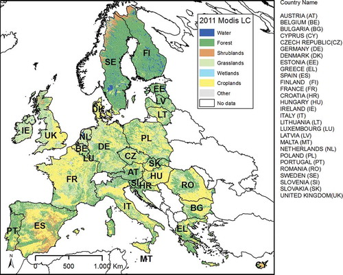
Figure 1. 2011 MODIS LC mosaic as produced after mosaicking and reclassification. Countries are listed in alphabetical order based on abbreviation. For full colour versions of the figures in this paper, please see the online version.

Forest and cropland are two LC classes vital for humans. Apart from its beneficial role in the global carbon cycle, economic growth, and recreational activities, forest represents some of the most diverse ecosystems on earth containing most of the living species (e.g., 90% of the planet’s species live in tropical forests; FAO 2010). Cropland provides 99.7% of the global human food supply, while the rest 0.3% comes from the sea (Day et al. 2014). Forest and cropland LC classes are dynamically changing mostly due to human actions (Lambert et al. 2013). These transformations have been described as being among the main drivers of global environmental changes that threaten earth’s sustainability (Lambin and Meyfroidt 2011; Unger 2014). For example, clearing land to create new croplands and intensifying existing croplands to meet the needs for increased crop production account for about a quarter of global greenhouse gas emissions (Tilman et al. 2011). In addition, the conversion of forests into croplands in the last 150 years worldwide has led to reduced net global cooling of about 0.1°C (Unger 2014). This does not suggest that increased forest loss is beneficial for climate change, but it highlights climate’s complexity (Unger 2014). Forest and cropland transformations are also affected by overpopulation (Lutz et al. 2012). As population increases, so do their resource needs for food, water, materials, and natural resources leading to either a conversion from one LC class to another (e.g., forest to cropland), or to the intensification use of already existing areas, or to both (Jarnagin 2006). The expected population increase will continue to pressure earth’s natural resources with even higher demands, thus a comprehensive strategic plan is needed.

Along these lines, the 2012 Rio+20 UN Conference on Sustainable Development recognized in its resolution entitled “The future we want” the importance for the “safeguarding of land resources” and the need for increased initiatives and scientific studies aimed at “deepening understanding and raising awareness of the economic, social and environmental benefits of sustainable land management and policies” (UN 2012a). It also highlighted the necessity for promoting and supporting more sustainable agriculture (including crops), increasing food security and forestry, while conserving land, biodiversity, and ecosystems (UN 2012b). In the same context, the UN recognized the importance of geospatial technologies for global LC mapping through satellite data and their use along with other socioeconomic variables to “facilitate informed policy decision-making on sustainable development issues” (UN 2012b). Although numerous and complex interactions exist between socioeconomic characteristics and various LC types, limited studies exist relating forest and cropland LC classes to socioeconomic variables (Grekousis and Mountrakis 2015). Integrating socioeconomic indices and variables with LC data should be put at the center of the research agenda to identify subpopulations that contribute at a higher or lower degree to sustainable development (Grekousis, Mountrakis, and Kavouras 2015; Lutz et al. 2012; Szantoi et al. 2012).

Linking “people to pixels” or “socializing the pixel” provides a geographic context in social behavior offering more possibilities to assess the impact of humans on land resources (Livermore et al. 1998; Butz and Torrey 2006; Lambin et al. 2009; Propastin and Kappas 2012). Spatial analysis of human settlement patterns, population change, and future trends along with consumption and behavioral patterns are considered of primary importance in understanding environmental and climate changes (O’Neill, MacKellar, and Lutz 2001; Butz and Torrey 2006; Forbes 2013). For example, the linkage of geography and macroeconomics might provide explanations for how much of the regional differences in per capita output are due to geography or a country’s specific factors such as institutional differences (Nordhaus 2006). The integration of socioeconomic variables in environmental research might explain why some regions inside a country or some countries compared to others lag environmentally.

Inspired by the aforementioned concepts, in this paper, land-related data were coupled with socioeconomic information for the 28 member countries comprising the European Union (EU28) to assess the human impact on land resources by identifying relations among them. First, the LC status for EU28 for the year 2011 was calculated. Forest and cropland estimations were then coupled with socioeconomic characteristics related to real gross domestic product (GDP), urbanization, and human/environmental quality. EU28 offers a highly heterogeneous land and socioeconomic landscape responding to different national pressures, making this an interesting comparison, beyond the obvious land size (Grekousis, Kavouras, and Mountrakis 2015). The rest of the paper presents the materials and methods (section 2) followed by results (section 3). Section 4 presents discussion and conclusions.

Materials and methods

Forest and cropland land cover estimation for 2011

Forest and cropland estimations were based on the moderate resolution imaging spectoradiometer (MODIS) global land cover type product, or MCD12Q1, which supplies annual global LC maps at 500-m spatial resolution (Schneider, Friedl, and Potere 2010; Friedl et al. 2010; NASA 2013). The MODIS database provides LC data from 2001 through 2013. In order to be consistent with the socioeconomic data referring to 2011, MODIS data were selected for the reference year 2011. To fully cover the EU28 spatial extent, 14 tiles were mosaiced, each one consisted of 2400 × 2400 (rows/columns) covering approximately 1200 × 1200 km with an 8-bit unsigned integer data type. The primary LC scheme associated with the MODIS LC product was used, which consisted of 17 LC classes defined by the International Geosphere-Biosphere Programme (IGBP; Loveland and Belward 1997), at 500-meter pixel size. While this pixel size is relatively large, super-resolution techniques, where a coarse pixel percent cover is distributed spatially at a higher resolution, have not yet gained importance for widespread usage (Jin, Mountrakis, and Li 2012). The user and producer accuracies are greater than 70% for this classification (Friedl et al. 2010). Administrative boundaries for the EU28 countries expressed as polygons were incorporated using the ETRS89 coordinate reference system for the 2010 reference year at 1:3M scale (Eurostat 2014a).

To produce the 2011 forest and cropland maps, a typical geographic information system (GIS) procedure was followed, where the 14 MODIS raster data sets were first merged and then reclassified to reduce the 17 classes, which the MODIS data set comes with, to 7 classes of wider interest from the environmental policy perspective (Table 1). Using zonal statistics, the total number and percent cover of forest and cropland pixels were calculated inside the boundaries of each country.

Table 1. EU28 LC classes and reclassification.

MODIS IGBP		Reclassified EU28 LC classes
Name	Class code	Name	Class code
Water	0	Water	1
Snow and ice	15
Evergreen needleleaf forest	1	Forest	2
Evergreen broadleaf forest	2
Deciduous needleleaf forest	3
Deciduous broadleaf forest	4
Mixed forest	5
Woody savannas	8
Savannas	9
Closed shrublands	6	Shrublands	3
Open shrublands	7
Grasslands	10	Grasslands	4
Cropland/natural vegetation mosaic	14
Permanent wetlands	11	Wetlands	5
Croplands	12	Croplands	6
Urban and built-up	13	Other	7
Barren or sparsely vegetated	16

Socioeconomic variables and analysis

For the socioeconomic analysis, it was necessary to adjust for a wide-ranging population size per country. Population was provided by Eurostat, as the inhabitants of a country at the NUTS0 geographical level, on 1 January 2011 (Eurostat 2014b). Eurostat based this information on the data from the most recent census, and then adjusted the numbers using post-census population changes and population registers. Population is used to calculate the forest and cropland area per capita for the EU28 countries. Forest per capita can be used as an indicator for resource potential, revealing the limits to forest resources availability (Woodall and Miles 2008) or how forest rich or forest poor a country is. Due to the heavy population pressure on resources, the low per capita forest area reveals a shortage in forest resources. Cropland per capita represents the land in hectares where food can be grown per person. Cropland per capita assesses the pressures on land resources due to the increasing demand for food (Zoebisch and Pauw 2006; Ramankutty, Foley, and Olejniczak 2008; Tilman et al. 2011). For example, although dependent on different factors (e.g., location, technology, etc.), it is estimated that the minimum cropland per capita area needed to produce an adequate quantity of food is 0.1 ha (Engelman and LeRoy 1995).

Moving beyond the population normalization, five socioeconomic indicators were implemented linking human behavior and environmental footprints. These indicators included (a) real GDP per capita as an economic indicator revealing economic development, (b) urbanization degree (UD) expressed as the percentage of people living in cities, (c) Human Development Index (HDI) as a measure of human prosperity through a combination of income, health, and education, (d) ecological footprint (EF) measuring human consumption of natural resources, and (e) total biocapacity (TB) expressing the earth’s ability to offer these resources in a sustainable way. Although these variables and indices have received criticism regarding their ability to fully depict what they are designed to show (Ewing et al. 2010), they still offer a baseline for a general discussion. A detailed description of each indicator is given below.

• Real GDP per capita: It is the final result of the production activity in euros per inhabitant and was obtained from Eurostat at the NUTS0 geographical level (Eurostat 2014b). Verma, Betti, and Gagliardi (2010) provided a survey on error assessment for Eurostat’s Income and Living Conditions. Three different approaches of GDP calculation are used by the national EU member statistical offices (GDP output approach, GDP expenditure approach, and GDP income approach) (Eurostat 2014b). For this reason, results are then balanced by Eurostat, so that a single value for GDP is obtained. Specific methodologies, data treatment, classifications, definitions, quality, and the statistical production processes for national population and GDP per capita can also be found in the metadata file associated with each table in the database. The real GDP per capita is used as an indicator of how well off a country is since it is the ratio of real GDP (real income) to the average population of a specific year in that country (for simplicity, the term GDP pca is used in this study) (Eurostat 2014b). GDP pca has been linked to land dynamics as higher GDP per capita and the increasing affluence is often regarded as a significant driver for the increased human footprint for biologically productive land, being thus one of the main causes of biodiversity loss (Weinzettel et al. 2013).

• Urbanization degree: Per country urban population for 2011 was obtained from the UN Food and Agriculture Organization (FAO) statistics (FAOSTAT 2013). As the MODIS data set does not include a built-up related LC class for the year 2011, the ratio of urban population to total population (urban and rural populations combined) of each country was used, which is the percentage of people living in cities (urbanization degree) (1).

  (1)

  where is the urbanization degree, taking values in the space [0,1], is the urban population, and is the rural population of a country. The magnitude of the people living in urban environments (as a percent of the total population), and the impact of urban sprawl have been associated with transformational effects to other LC classes such as forest, agriculture, and water (Alig, Kline, and Lichtenstein 2004; Jarnagin 2004; White, Morzillo, and Alig 2009; Grekousis and Mountrakis 2015).

• Human Development Index: The HDI for 2011 was retrieved from the UN Development Programme (UNDP 1990, 2014). It is a summary measure that takes into account health conditions through life expectancy at birth (Index Life), educational attainment through mean and expected years of schooling (Index Education), and general economic status through the gross national income (GNI) per capita (Index Income). The HDI is the geometrical mean of the three dimension indices (2) (Klugman, Rodríguez, and Choi 2011):

(2)

Although the HDI does not reflect on inequalities, security, or poverty, it is used in the work as an expression of the levels of social and economic development for a given country. The HDI is expressed as a value from 0 to 1, from least to most developed countries with values over 0.8 labeled as “very high” and values between 0.69 and 0.80 labeled as “high.” The HDI has been used as a strong, sustainable indicator based on the idea that high human development is closely related to sustainability (Wilson, Tyedmers, and Pelot 2007).

• Ecological footprint: The EF was obtained for the year 2011 from the Global Footprint Network (GFN) through the National Footprint Account 2015 database (GFN 2015). Borucke et al. (2013) provided the calculation methodology for the 2011 edition of the National Footprint Accounts (3):

  (3)

  where P is the amount of each primary product i harvested or waste emitted in the nation, Y_N,i is the average yield for product P, and YF_N,i and EQF_i are the yield factor and the equivalence factor, respectively, for the country and LC in question. Five main LC types are used for the calculation of EF: built-up land, forestland, fishing ground, cropland, and grazing land. EF is measured in global hectares. One global hectare is the world’s average productivity area of land and water for a given year. The EF calculates the land and water area per capita needed to produce all the resources a population consumes and requires to absorb its waste (Wackernagel et al. 2002; Ewing et al. 2010). It represents the demand on land and the portion of the planet’s regenerative capacity (actual biocapacity) used by certain human activities. The EF is regarded as one of the most important indices in the evaluation of sustainability (Siche et al. 2008).

• Total biocapacity: The TB indicator was obtained for the year 2011 from the GFN and is also measured in global hectares (GFN 2015). It represents the supply, or the amount of productive land available to generate the resources that humans need and to absorb the waste (Ewing et al. 2010). A country’s TB is calculated as follows (4) (Borucke et al. 2013):

  (4)

  where A_N,i is the bioproductive area (land area) that is available for the production of product i of each nation and YF_N,i and EQF_i are the yield factor and the equivalence factor, respectively, for the country and associated LC. This measure does not take into account any other species consuming the same biological material as humans. TB can be compared with EF and ecological deficit or reserve may be tracked by subtracting the supply (TB) from the demand (EF) (EEA 2014). EF and TB were not available for Malta and Luxembourg for the year 2011.

To identify any statistically significant correlations and highlight the related linkages among the forest per capita, cropland per capita, GDP per capita, the UD, the HDI, the EF, and the TB, Pearson’s correlation coefficients were calculated. Correlation analysis has been used in several studies related to LC types and various variables/indicators (Eva and Lambin 2001; Wyman and Stein 2010; Zhou, Huang, and Cadenasso 2011; Bagan and Yamagata 2015). To better control for economic development differences, countries were aggregated into three economic groups (low, moderate, and high) based on their GDP per capita. Scatter plots, correlation analysis, and boxplots are used to see if distributions of the forest per capita, cropland per capita, forest share, and cropland share vary between different economic groups. To test if distributions are statistically significantly different, the Mann–Whitney U test was applied (Mann and Whitney 1947; Nagendra, Pareeth, and GHate 2006; Grekousis and Mountrakis 2015). Hypothesis to be tested was: economic development does not affect the median values for the forest per capita, cropland per capita, forest share, and cropland share. Three significance levels for α (0.05, 0.01, and 0.001) were selected and if the p-values resulting from the test were to be less than α, then there would be compelling evidence to reject the hypothesis and conclude that these two distributions have statistically significant differences. This would conclude that economic development affected the variable at hand.

In addition, simple linear fits are used to model UD with forest and cropland and make assessments regarding future trends for forest and cropland in relation to urbanization dynamics. Analysis and conclusions are based in the space for time substitution technique, which assumes that spatial and temporal variations are equivalent and thus one can infer a temporal trend by studying sites of different locations (Pickett 1989; Blois et al. 2013). The space for time substitution technique is mostly used in ecological studies, when there is a lack of historical data and general trends are investigated or when hypotheses are to be generated (Pickett 1989). Although this technique has certain limitations, many studies base their outputs on space for time substitution (Arago et al. 2010; Blois et al. 2013; Grekousis and Mountrakis 2015).

To compare results at the global scale and provide wider discussion, world average values for the forest area per capita (FAO 2010), cropland area per capita (World Bank 2015), the percentage of forest coverage worldwide, and the percentage of cropland coverage worldwide (World Bank 2015) were also included in the analysis. The FAO and the World Bank have different ways of calculating and defining LC classes than MODIS. For example, the World Bank uses the term agriculture for land that is arable, under permanent crops, and under permanent pastures, but MODIS uses a specific class for cropland (Friedl et al. 2010; World Bank 2015). While the MODIS results for the above measures are likely to be different if calculated, the world averages can provide a general qualitative comparison metric.

Results

Forest and cropland distribution within EU28

Before examining the correlation of forest and cropland to socioeconomic indicators, it is helpful to understand forest and cropland distribution. The MODIS LC mosaic for the year 2011 is presented in Figure 1. LC varies among the EU28 countries depending on the geographical location and the different landscape. Figure 2 depicts major LC proportions for each EU28 country, while Figure 3 focuses on the geographic distribution of the LC classes of interest: forest and cropland. To build Figure 2, forest share and cropland share data were used, as produced from the MODIS mosaic for the year 2011 after the reclassification of the initial data set and calculation of zonal statistics by overlaying the boundaries of EU28 countries. Forest is the most dominant class covering 40.4% of the total EU28 area compared to 30.2% for croplands, 21.2% for grasslands, 3.6% for shrublands, 1.9% for water, 0.3% for wetlands, and 2.4% belonging to other LC types. Forest has strong presence in Northern Europe (e.g., Finland with 82.6% and Sweden with 75.5%), while in southern countries (e.g., Cyprus, Malta, France, and Spain), it does not exceed 35%. For comparison, the 2011 world forest average is estimated at 30.9% (World Bank 2015). In terms of cropland share, Hungary is the leading country with 63.2% followed by Denmark (59.7%), France (48.0%), and Romania (45.7%). The lowest shares are recorded in Finland (0.6%), Sweden (2.0%), and Ireland (3.6%). The 2011 world cropland average is estimated at 37.6% (World Bank 2015).

Figure 2. 2011 LC share per country for the EU28. EU28 average is also plotted for comparison.

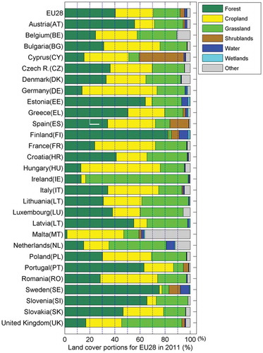
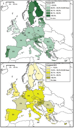
Figure 3. Forest and cropland shares for EU28 in 2011. The EU28 mean value for forest and cropland share is used in the legend as class boundary to better track EU28 countries above or below the mean.

Forest per capita and cropland per capita

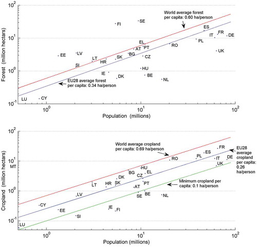
To better control for population differences, forest and cropland area were adjusted with each country’s population, calculating the forest per capita and cropland per capita (Figure 4). Countries below the EU28 average lines have lower forest per capita and cropland per capita areas than those above the EU28 average lines. The per capita forest area at the global scale for 2010 is 0.60 ha (FAO 2010). The average forest area per capita in EU28 for 2011 is 0.35 ha (40% less than world average). The World Bank (2015) reported the world average cropland per capita for the year 2011 to be 0.69 ha, and in our analysis, the EU28 average is 0.26 ha. No EU28 country exceeded the world average cropland per capita. However, four northern EU28 countries (Finland, Sweden, Latvia, and Estonia) far exceeded the 0.60 ha forest per capita world average and are the EU28 forest richest countries, with more than 1.70 ha per person each, which is five times more than the EU28 average (0.35 ha per capita). These countries are regarded as forest outliers. Cropland outliers are not detected.

Figure 4. Log–log plot of forest and cropland in million hectares against population in millions for the year 2011. The diagonally solid lines represent the EU28 average in forest and cropland per capita and dashed red lines represent the global average in forest and cropland per capita. The green line represents the minimum cropland per capita (Engelman and LeRoy 1995).

Based on the correlation coefficients at the EU28 level, forest per capita has a strong positive correlation with the TB (r = 0.88) and a moderate correlation with the EF (r = 0.43; Table 2). On the other hand, forest per capita is not correlated with the GDP per capita, the UD, or the HDI. If the four richest forest per capita countries (Finland, Sweden, Latvia, and Estonia) are excluded, then the correlation between forest per capita and UD is moderate negative (r = −0.69), and the correlation between forest per capita and the TB is weak positive (r = 0.12). Results are also different between the forest per capita and the GDP per capita, in which there is a negative moderate correlation (r = −0.42), but not statistically significant. For this reason, special attention should be given when referring to correlations of forest per capita with other variables, because in the case of using the EU28 set, there is a possibility to lead to incorrect conclusions (e.g., forest per capita is irrelevant to UD). Cropland per capita has negative weak correlation with the forest per capita (r = −0.24), the UD (r = −0.27), and the TB (r = −0.20), and moderate negative correlation with the GDP per capita (r = −0.53), the HDI (r = −0.61), and the EF (r = −0.61).

Table 2. Pearson’s correlation coefficient. Asterisk (*) indicates correlations statistically significant at the p < 0.01 level. p-Value is the probability of getting a correlation as large as the observed value by random chance, when the correlation is zero (null hypothesis). Forest outliers: Estonia, Latvia, Sweden, and Finland. (GDP: gross domestic product; pca: per capita; UD: urbanization degree; HDI: Human Development Index; EF: ecological footprint; TB: total biocapacity).

	Forest pca	Cropland pca	GDP pca	UD	HDI	EF	TB
Forest pca	1	−0.24	0.06	0.11	0.06	0.43	0.88*
Cropland pca		1	−0.53*	−0.27	−0.61*	−0.61*	−0.20
GDP pca			1	0.54*	0.80*	0.54*	0.21
UD				1	0.45	0.44	0.20
HDI					1	0.56*	0.05
EF						1	0.57*
TB							1
Forest pca without outliers	1	−0.31	−0.42	−0.69*	−0.40	−0.21	0.12

GDP per capita

The GDP per capita has a moderate positive correlation with the UD (r = 0.54) and the EF (r = 0.54) (Table 2). In addition, the GDP per capita has a strong correlation with the HDI (r = 0.80), expected to some extent, as the HDI includes gross national income per capita in the calculation.

For better delineation of the economic groups, the average EU28 GDP per capita (23,400 euros per capita, Table 3; Eurostat 2014b) was rounded to the next thousand (24,000 euros per capita). On the basis of the fact that the at-risk of poverty threshold for the year 2011 is not exceeding 12,000 euros per capita for each one of the EU28 countries (with the exception of Luxembourg and Austria) (Eurostat 2014b), those having less than 50% of EU28 GDP per capita (12,000) are labeled “low GDP per capita countries.” Countries having a GDP per capita larger than the EU28 GDP per capita average are labeled “high GDP per capita countries” and countries in between these values are labeled “moderate GDP per capita countries.”

Table 3. Average values for the three economic groups, EU28 and worldwide. (*) Data not available. Values in parentheses in forest per capita and forest share have been calculated removing forest-rich outlier countries. Values for the HDI, the EF, and the TB for the economic grouping are not offered from GFN.

Group	Forest pca (ha)	Cropland pca (ha)	Urban population (%)	Forest share (%)	Cropland share (%)	HDI	EF	TB	GDP pca
Low	0.36(0.30)	0.41	62.12	33.04(30.21)	38.05	*	*	*	7592
Moderate	0.31(0.31)	0.28	70.20	39.22(39.22)	35.80	*	*	*	20,943
High	0.36(0.14)	0.19	80.02	44.61(25.87)	23.61	*	*	*	30,399
EU28	0.35(0.22)	0.26	73.78	40.36(31.16)	30.23	0.86	4.1	2.3	23,400
World	0.60	0.69	52.00	30.80	37.61	0.70	2.7	1.7	*

To investigate if geographical patterns exist among GDP per capita, forest per capita, and cropland per capita, the GDP grouping and the EU28 countries are overlaid (Figure 5). There is a strong geographical pattern in GDP grouping because low GDP per capita countries are located in Eastern Europe, moderate GDP per capita countries are located next to the Mediterranean Sea, and high GDP per capita countries are located in Central and Northern Europe.

Figure 5. Forest area per capita and cropland area per capita for 2011. Three GPD per capita economic groups are also overlaid. EU28 mean value for forest per capita and cropland per capita is used as class boundary to better track which EU28 countries lie above or below this value. First class is less than 1 mean value, second class is 1–2 mean values, and third class is more than 2 mean values.

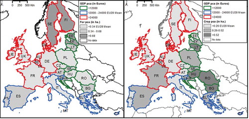
For the EU28 level, forest per capita follows the GDP per capita distribution as the average forest per capita per group is near the EU28 average (Tables 3, 4 and Figures 5, 6). For example, the four most forest-rich per capita countries (Sweden, Finland, Estonia, and Latvia) have more than 1.7 ha of forest area per capita and belong to two different economic groups. Sweden and Finland belong to the high GDP per capita countries, with more than 31,000 euros per capita, while Estonia and Latvia belong to the low GDP per capita countries, with less than 9000 euros per capita. This is actually a result of the geographical location because a northern country is most likely to be forest rich regardless of the GPD per capita. On the other hand, the Mann–Whitney U test reveals that there is no statistically significant difference in distributions among groups for the forest per capita and forest share (Tables 3, 4 and Figure 6). Therefore, in general, it cannot be concluded from the above data set that the forest per capita and the forest share are linked to GDP per capita. However, by the exclusion of the forest outliers (Finland, Sweden, Latvia, and Estonia), the results differ significantly (Figure 6). In this case, there is a statistically significant difference between high GDP per capita countries and low GDP per capita countries for forest per capita. High GDP per capita countries have, on average, 0.14 ha forest per capita, which is almost half the forest per capita (0.30 ha) of the low GDP per capita countries. This trend is slightly shown in forest share as well, as the average value of high GDP per capita countries is 15% smaller than low GDP per capita countries and 35% smaller than moderate GDP per capita countries. This trend is also depicted in Figure 7 (more comments can be found in the “Urbanization Degree” section). Still, the Mann–Whitney U test reveals no statistically significant differences among the economic groups regarding forest share.

Table 4. p-Values for the Mann–Whitney U test for the three economic groups. Values in parentheses in forest per capita and forest share have been calculated removing forest-rich outlier countries.

p Values	Forest pca	Cropland pca	Forest (%)	Croplands (%)
Low–moderate	0.4306 (0.8870)	0.1541	0.8125 (0.4634)	0.8867
Moderate–high	0.6426 (0.1995)	0.3817	0.7242 (0.2523)	0.2462
High–low	0.0977 (0.0138)	0.0027	0.5494 (0.3213)	0.1926

Figure 6. Boxplots for all variables over the three economic groups. Each boxplot includes median, 25th, and 75th, percentiles (marked by upper and lower edges of boxes). Red horizontal dashed lines express average for each economic group. The red lines represent EU28 and EU24 average value and the blue lines represent the world average value. *: 0.01 < p ≤ 0.05, **: 0.001 < p ≤ 0.01, ***: p ≤ 0.001, NS: p > 0.05.

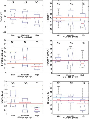
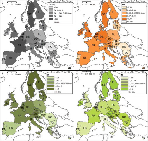
Figure 7. SE variables geographic distribution for the EU28.

Cropland per capita is unevenly distributed regarding GDP per capita (Table 3, Figure 6). On average, low GDP per capita countries have almost twice the cropland LC per capita (0.41) compared to high GDP per capita countries (0.19) (statistically significant difference), which is less than the EU28 average (0.26). On average, the moderate GDP per capita group has almost one-third less cropland LC per capita (0.28) compared to the low GDP per capita group, but their differences in median values are not statistically significant. For the cropland share, there are no statistically significant differences among economic groups, yet for the high GDP per capita countries (23.61%), it is 20% smaller than the EU28 average (30.23%) (Table 3, Figure 6).

Urbanization degree

High UD can be found mainly in northern countries, for example, France, Belgium, or the Netherlands (Figure 7, Table 5). These countries have at the same time low values in forest share. On the other hand, countries with low UD values, for example, Romania or Slovenia, have higher values in forest share. This trend is also evident in Figure 8, which illustrates the forest share and the cropland share with UD along with economic development, using the three GDP per capita groups. The general view for the EU28 countries for the forest share over UD reveals a negative trend, as when the urban population share increases, the forest share decreases. The high GDP per capita countries (with the exception of the two forest richest countries of Finland and Sweden) are mainly grouped in the lower right corner of the figure. These countries have 10% more people living in their cities compared to the EU28 average, and their forest share (25.87%) is almost 40% less than that of the EU28 (Table 3). The negative trend of forest share to urban population share is more evident within the moderate GDP per capita countries because these countries seem to be aligned within a sharp negative slope with a correlation r = −0.89. The linear fit model is applied to the moderate GDP per capita group having an R² = 0.79 and an R² adjusted = 0.75. This linear fit model reveals that for the moderate GDP per capita group, a 5.0% increase in urban population will lead to a 7.4% decrease in forest share. For forest share data, linear fit models are not depicted for low and high GDP per capita groups, as well as for the total set of EU28 countries as they have R² < 0.08.

Table 5. Socioeconomic values, forest and cropland shares, and per capita values per country.

NAME	NUTS_ID	UD (%)	HDI	EF	TB	GDP pca	Economic group	Forest pca (HA)	Cropland pca (HA)	Forest (%)	Croplands (%)
Austria	AT	67.65	0.88	5.13	3.15	32,100	3	0.55	0.16	55.69	15.88
Belgium	BE	97.48	0.88	5.77	1.14	29,800	3	0.07	0.09	24.64	33.07
Bulgaria	BG	73.12	0.77	2.64	2.93	3700	1	0.47	0.67	31.11	44.85
Cyprus	CY	70.40	0.85	3.59	0.35	18,100	2	0.17	0.39	15.50	35.57
Czech Republic	CZ	73.41	0.86	4.50	2.58	11,600	1	0.27	0.25	36.36	33.36
Germany	DE	73.93	0.91	4.37	2.06	30,000	3	0.14	0.14	33.04	31.68
Denmark	DK	86.94	0.90	4.28	4.49	37,500	3	0.11	0.46	13.89	59.73
Estonia	EE	69.50	0.84	5.46	9.94	9100	1	2.17	0.18	64.25	5.26
Greece	EL	61.44	0.85	3.91	1.49	15,900	2	0.60	0.35	50.49	29.18
Spain	ES	77.42	0.87	3.41	1.49	20,600	2	0.37	0.41	34.29	38.03
Finland	FI	83.69	0.88	4.84	13.19	31,300	3	5.15	0.04	82.58	0.64
France	FR	85.82	0.88	4.16	2.94	27,800	3	0.20	0.41	23.97	48.41
Croatia	HR	57.79	0.81	3.20	2.70	8600	1	0.54	0.32	41.14	24.44
Hungary	HU	69.46	0.82	2.81	2.35	8900	1	0.12	0.59	12.95	63.23
Ireland	IE	62.19	0.90	4.64	3.82	36,500	3	0.20	0.05	13.17	3.55
Italy	IT	68.38	0.87	4.15	1.08	23,500	2	0.17	0.20	34.36	40.52
Lithuania	LT	67.08	0.83	4.38	4.24	7700	1	0.65	0.65	30.81	30.69
Luxembourg	LU	85.47	0.88	4.10	2.30	64,200	3	0.19	0.11	38.16	22.09
Latvia	LV	67.68	0.80	5.58	8.75	6400	1	1.71	0.32	55.12	10.46
Malta	MT	94.84	0.82	4.10	2.30	13,400	2	0.00	0.03	1.85	45.12
Netherlands	NL	83.18	0.91	4.45	1.11	33,200	3	0.03	0.05	15.13	20.18
Poland	PL	60.85	0.83	3.83	1.97	8300	1	0.24	0.31	30.23	38.86
Portugal	PT	61.06	0.82	3.34	1.51	14,700	2	0.53	0.20	63.19	23.57
Romania	RO	52.80	0.78	2.50	2.61	4300	1	0.33	0.54	28.33	45.69
Sweden	SE	85.20	0.90	6.51	10.54	35,200	3	3.58	0.10	75.45	2.03
Slovenia	SI	49.90	0.87	4.53	2.33	15,400	2	0.65	0.07	65.60	7.41
Slovakia	SK	54.73	0.83	3.78	2.81	9200	1	0.42	0.29	46.62	32.14
United Kingdom	UK	79.46	0.89	4.15	1.37	30,600	3	0.07	0.11	16.85	28.58
EU28	EU28	73.80	0.86	4.10	2.30	24,000	3	0.35	0.26	40.30	30.20
World	WORLD	52.00	0.70	2.65	1.72		3	0.60	0.69	30.87	37.59

Figure 8. LC shares over UD and GDP per capita groups.

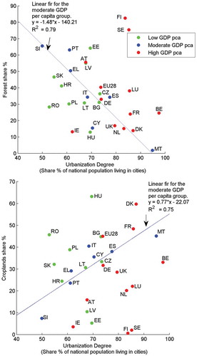
Cropland share at the EU28 level is weakly correlated with urban population share having a random distribution. Yet, for the moderate GDP per capita countries, there is a clear positive correlation (r = 0.86) between the cropland share and the urban population share, and the linear fit model applied has an R² = 0.75 and an R² adjusted = 0.70. Model reveals that for the moderate GDP per capita group, a 5.0% increase in urban population will lead to a 3.9% increase in cropland share. This highlights (and will be further discussed in the discussion and results section) that these countries have a trend for increase in land dedicated for agricultural needs when urbanization increases, possibly due to their economic structure, despite the fact that their cities are getting larger. Linear fits for low and high GDP per capita groups are not depicted as they have R² < 0.09.

HDI

There is a high level of human well-being as 26 of the studied countries have a very high HDI and all of them have more than the 2011 global average HDI (Tables 3 and 5, Figures 8 and 9). Still countries having the lowest values in the EU28 are clustered (with the exception of Portugal) in Eastern Europe, for example, Bulgaria, Romania, Hungary, or Slovakia, having at the same time high values in cropland per capita (Figure 8). Looking at the EU28 level, HDI is uncorrelated to forest per capita (r = 0.06), but if outliers (Finland, Sweden, Latvia, and Estonia) are not included, then the correlation is moderate negative (r = −0.40; Figure 9, Table 2). In addition, the economic grouping appears to create a clear cluster for the high GDP per capita countries that are mostly concentrated on the lower right part of the graph, meaning that the more affluent countries tend to have smaller forest LC per capita values, which is less than half that of the EU28 average.

Figure 9. Forest per capita and cropland per capita over the HDI, the EF, and the TB.

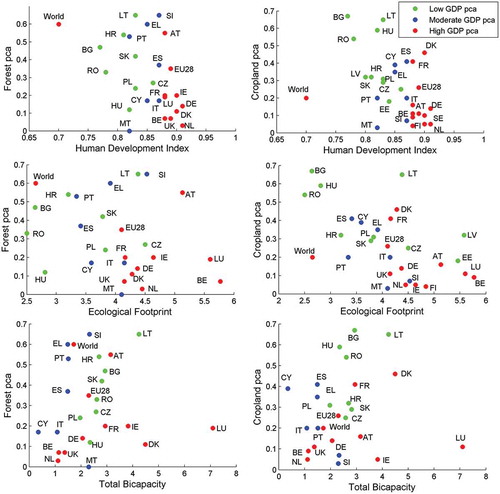
Cropland per capita has a moderate negative correlation (r = −0.61) with the HDI and most of the high GDP per capita countries are clustered in the lower right corner of the graph (Figures 6 and 9). The negative correlation is also present in the low GPD per capita countries. Moderate GDP per capita countries lie in between the two other groups. This graph clearly shows that the more affluent countries (Denmark, Netherlands, and Finland) base their economies on non-primary sectors of the economy, possibly the tertiary economic sector. The low GDP per capita countries, such as Bulgaria, Romania, and Hungary, have large values in cropland per capita, which aligns with the general idea that countries with lower incomes tend to base their economies on the primary sector, making direct use of their natural resources.

EF

High values in EF can be found in Northern Europe and especially in Scandinavian and Baltic countries (Figure 7). Forest per capita with the EF is weakly correlated (r = −0.21), and high GDP per capita countries tend to be in the lower right part of the graph. The cropland LC per capita has a moderate negative correlation (r = −0.61) with the EF, but economic groups are not that distinct (Figures 6, 9). The average EF per capita for EU28 is 4.1 global hectares, much higher than the global average of 2.6 global hectares per capita. Residents of Romania have the lowest EF, at 2.5 global hectares per capita, which is even less than the global average. On the other hand, Sweden lies on the first position of the rank, being the country with triple EF compared to world average. EU28 has an ecological deficit of 1.8 global hectares per capita from the EU28 average biocapacity per person for 2011 (Table 3) (EF–TB average values, GFN 2015).

TB

High values in TB are clustered in Northern Europe and especially in Scandinavian and Baltic countries, while Mediterranean countries tend to have the lowest values in TB (Figure 7). Forest per capita with TB has weak correlation (r = 0.12). Still, in this graph, there is a clear distinction of low and moderate GDP per capita countries. They both tend to have a sharp increase in forest per capita when the TB increases, but moderate GDP per capita countries are on the far left of the graph, having a nearly constant distance from the low GDP per capita countries of around 1 global hectare for similar forest per capita values. Also, high GDP per capita countries tend to cluster closer to low GDP per capita countries and further away from the moderate GDP countries. This is strange because there seems to exist a clear structure between low and moderate GDP per capita groups, and the high GDP per capita group is more freely scattered. Finally, the cropland LC per capita compared with the TB has a weak negative correlation (r = −0.20) and clear patterns are not recognized.

Discussion and conclusions

The well-being of a society is clearly linked to the natural resources and the biological capacity available to that society. The unbalanced economic growth and human prosperity at the expense of nature’s stability are shortsighted as the consequences of ecological degradation that usually follow with a time lapse are often irreversible. Timely and accurate LC information is essential for monitoring the environment. When coupled with socioeconomic indices and variables, it can locate subpopulations, habits, or trends that affect environmental and climate change at different levels and degrees, enabling quicker policy decisions, regulatory actions, and measures, if needed, for a more sustainable future.

Currently, various metrics, sustainable indices, and extensive LC databases are available, offering a clear status of the European natural landscape for succeeding in sustainable development. In this research, the EU28 LC status for 2011 was presented, and forest and cropland LC classes were further analyzed with various socioeconomic variables to reveal any linkages with the population (forest per capita and cropland per capita), economic development (GDP per capita), urban development (UD), human prosperity (income, health, and education; HDI), the way humans consume natural resources to satisfy their needs (EF), and the ability of earth to offer these resources in a sustainable way (TB). The key findings of the research for every SE variable related to forest and cropland LC are presented below:

Forest LC: The average forest area (0.35 ha) per capita in EU28 is almost half that of the world average forest (0.60 ha) per capita.

• GDP: Excluding forest outlier countries, forest per capita average is negatively correlated to GDP per capita (r = −0.42). Compared to low GDP per capita countries, high GDP per capita countries have 50% less forest (0.14 ha) per capita. This makes high GDP per capita countries forest poor for their citizens.

• UD: Excluding forest outlier countries, forest per capita average is negatively correlated to UD (r = −0.69). Countries with high percentage of people living in cities have lower forest share. For example, most of the countries that have more than 80% of the national population living in their cities are high GDP per capita countries, having 40% less forest share than that of the EU28 average. The negative correlation among the urban population and forest share is even larger within the moderate GDP countries with r = −0.89. A 5.0% increase in urban population will lead to a 7.4 decrease in forest share for these countries, something that should be taken into account during planning in order to achieve a sustainable future. For example, smart growth policies should be in higher priority in these countries in order to save forest land resources during increasing urbanization.

• HDI: More affluent countries in terms of HDI tend to have smaller forest per capita values, which is less than half of the EU28 average.

• EF: EF is weakly negatively correlated to forest per capita (r = −0.21). Still, high GDP per capita countries tend to have high EF values and low forest per capita values (Figure 9).

• TB: Low and moderate GDP per capita countries tend to have a sharp increase in forest per capita when the TB increases. TB has a strong correlation with forest per capita only when forest outlier countries are included.

Cropland LC: The EU28 cropland per capita average is almost one-third of the world average cropland per capita, showing that cropland area is limited or possibly there is high agricultural productivity intensification.

• GDP: Cropland per capita average is negatively correlated to GDP per capita (r = −0.56). Low GDP per capita countries have more than double cropland (0.41 ha) per capita than high GDP per capita countries (0.19 ha). This is possibly explained by the fact that the more affluent countries base their economies on non-primary sectors of the economy.

• UD: Cropland share at the EU28 level is weakly correlated with UD. Still, for the moderate GDP countries, there is a strong positive correlation between the cropland share and the UD (r = 0.86). A 5.0 % increase in share of national population living in cities will lead to a 3.9% increase in cropland share. This is an interesting pattern, as it is at first sight contradictory to the general view that urbanization is mostly at the expense of agricultural land (Seto et al. 2011; Alig, Kline, and Lichtenstein 2004). It would be expected that the more urbanized a country is the less cropland share it has. For example, more than 3/4 of the artificial land uptake for the years 2000 through 2006 in the European area had previously consisted of arable and cropland LCs (EEA 2013). In this study though, the percentage of people living in cities was used and not the actual developed or built-up land share for defining urbanization. In addition, by using the percent value, the results were adjusted over the country’s population, and thus there were countries with similar UD values but with different populations in absolute values (e.g., Malta and Belgium), imposing different pressures on croplands when UD gets higher. The strong correlation of the moderate GDP per capita countries between UD and cropland share does not necessarily mean that new urban land does not come from croplands. This shows that there is an increase in agricultural needs, possibly due to the economic structure and higher standard of living. For example, Spain, Greece, Portugal, and Italy are all labeled as moderate GDP per capita with their economies being based to a large extent in agricultural goods and related exports. To suffice increased agricultural needs, new croplands might have been formed from other LCs. For example, 15% of new agricultural lands formed during 2000 to 2006 for Europe came from forests (EEA 2013). This might also explain why correlations between the forest share to UD and cropland share to UD for this economic group are almost identical but with opposite signs (r = −0.89 and r = 0.86; Figure 8).

• HDI: Cropland per capita has strong negative correlation with the HDI (r = −0.61) revealing that the more prosperous a society is the less cropland LC per capita it has.

• EF: Cropland per capita has strong negative correlation with the EF (r = −0.61) meaning that societies with high consumption rate tend to have smaller values in the cropland LC per capita.

• TB: TB is weakly negatively correlated with cropland per capita.

Concentrating people into cities and increasing urbanization does not necessarily mean that forest resources or agricultural lands are protected as a result of less land needed for dwelling and construction. On the contrary, there is a negative correlation between the forest shares and the UD which highlighted that the pressure of urban development led to the shrinking of forest land resources. Smart growth – as a response to cropland and forestland losses from the urbanization process – aims to create denser cities that are also attractive and comfortable, protecting forests, green spaces, and land resources. It is therefore important to improve urban monitoring methods (Mountrakis et al. 2009; Luo and Mountrakis 2010), develop accurate urban growth models (Wang and Mountrakis 2011; Grekousis, Manetos, and Photis 2013), and also connect modelers with urban planners (Triantakonstantis and Mountrakis 2012). For example, Finland and Sweden (Figure 7) succeed in this goal as they both have high shares in urban population and forest. The increase of the GDP per capita also threatens forests as high GDP per capita countries have smaller forest shares (Table 3). Sustainable development should be achieved by fulfilling both a very high HDI and a low EF within the earth’s limits, which is below the average biocapacity per capita value. The EU28 achieved a very high HDI in almost all of the participating countries; however, it was far away from being ecologically sustainable because it had a large ecological deficit (1.8 ghas, GFN 2015). If everyone in the world lived the average lifestyle of the Europeans, it would require almost two and a half (2.4) planet earths to meet their needs (GFN 2015). The road to development should advance human well-being, but only within the ecological limits of earth. The EU28 should make advances to further increase the HDI of mainly low GDP per capita countries, and at the same time follow a more ecologically friendly policy that will significantly save natural resources.

The EU also should take a more active role on the global scale as well. Taking into account overpopulation, the global average biocapacity per capita is expected to reduce further, which has been proven historically as global average biocapacity per capita has declined steadily from 3.2 ghas per capita in 1961 to 1.9 ghas in 2001 and 1.7 ghas in 2011 (GFN 2015). In addition, overpopulation and the expected increase in demand for biologically productive land to provide food, along with the increasing demand for fuels and construction materials (Lambin and Meyfroidt 2011), will put extra pressure on land systems, leading to rapid LC changes if left uncontrolled by economic forces. Many low-income countries in Asia, Africa, and Latin America typically have more sustainable land savings and ecological perspectives because they do not have an ecological deficit; however, they face the serious problems of hunger, poverty, disease, illiteracy, escalated urbanization, overpopulation, and political instability. These problems should be managed to reduce inequalities among countries and share human prosperity while pursuing earth’s ecological sustainability. After all, the availability of land and other natural resources is crucial for fighting hunger and poverty. Humans should pursue a balanced global increase of human prosperity and conserve natural resources, taking into account the long-term effects on the planet and the necessary legacy to be left to future generations.

Disclosure statement

No potential conflict of interest was reported by the authors.

Additional information

Funding

This work was supported by the State Scholarships Foundation of Greece (IKY) under Grant SR 22032/13, IKY Fellowships of Excellence for Postgraduate Studies in Greece–Siemens Program. Dr. Mountrakis’ research was partially supported by the National Aeronautics and Space Administration through a New Investigator Award [no. NNX08AR11G].

References

- Alig, R. J., J. D. Kline, and M. Lichtenstein. 2004. “Urbanization on the US Landscape: Looking Ahead in the 21st Century.” Landscape and Urban Planning 69: 219–234. doi:10.1016/j.landurbplan.2003.07.004.
- Aragao, L. E., and Y. E. Shimabukuro. 2010. “The Incidence of Fire in Amazonian Forests with Implications for REDD.” Science 328: 1275–1278. doi:10.1126/science.1186925.
- Bagan, H., and Y. Yamagata. 2015. “Analysis of Urban Growth and Estimating Population Density Using Satellite Images of Nighttime Lights and Land-Use and Population Data.” GIScience & Remote Sensing 52 (6): 765–780.doi:10.1080/15481603.2015.1072400.
- Blois, J. L., J. W. Williams, M. C. Fitzpatrick, S. T. Jackson, and S. Ferrier. 2013. “Space Can Substitute for Time in Predicting Climate-Change Effects on Biodiversity.” Proceedings of the National Academy of Sciences USA 110: 9374–9379. doi:10.1073/pnas.1220228110.
- Borucke, M., D. Moore, G. Cranston, K. Gracey, K. Iha, J. Larson, and E. Lazarus. et al. 2013. “Accounting for Demand and Supply of the Biosphere’s Regenerative Capacity: The National Footprint Accounts’ Underlying Methodology and Framework.” Ecological Indicators 24: 518–533, 1470–160X. doi:10.1016/j.ecolind.2012.08.005.
- Butz, W., and B. Torrey. 2006. “Some Frontiers in Social Science.” Science 312 (5782): 1898–1900. doi:10.1126/science.1130121.
- Day, J., M. Moerschbaecher, D. Pimentel, C. Hall, and A. Arancibia. 2014. “Sustainability and Place: How Emerging Mega-Trends of the 21st Century Will Affect Humans and Nature at the Landscape Level.” Ecological Engineering 65: 33–48. doi:10.1016/j.ecoleng.2013.08.003.
- EEA- European Environmental Agency. 2014. “Assessment of Global Megatrends — An Update Global Megatrend 2: Living in an Urban World.” Report. Accessed 25 February 2014. http://www.eea.europa.eu/publications/global-megatrends-update-2
- EEA-European Environmental Agency. 2013. “Changes in the European Land Cover Form 2000 to 2006.” Report. Accessed 25 February 2014. http://www.eea.europa.eu/data-and-maps/figures/land-cover-2006-and-changes-1
- Engelman, R., and P. LeRoy. 1995. Conserving Land: Population and Sustainable Food Production. Washington, DC: Population and Environment Program; Population Action International.
- Eurostat. 2014a. EuroGeographics for the administrative boundaries. Accessed 10 January 2013. http://epp.eurostat.ec.europa.eu/portal/page/portal/gisco_Geographical_information_maps/popups/references/administrative_units_statistical_units_1
- Eurostat. 2014b. Statistics database. Accessed 18 February 2014 http://epp.eurostat.ec.europa.eu/portal/page/portal/statistics/search_database. GDP per capita. Table code: nama_aux_gph Retrieved from: http://ec.europa.eu/eurostat/web/products-datasets/-/nama_aux_gph. Population: Table code: tps00001 Retrieved from: http://ec.europa.eu/eurostat/web/products-datasets/-/tps00001. At risk of poverty threshold: Code: tessi014
- Eva, H., and E. Lambin. 2001. “Fires and Land-Cover Change in the Tropics:A Remote Sensing Analysis at the Landscape Scale.” Journal of Biogeography 27 (3): 765–776. doi:10.1046/j.1365-2699.2000.00441.x.
- Ewing, B., D. Moore, S. Goldfinger, A. Oursler, A. Reed, and M. Wackernagel. 2010. The Ecological Footprint Atlas 2010. Oakland: Global Footprint Network.
- FAO. 2010. “Global Forest Resources Assessment 2010.” FAO forestry paper 163. Accessed 8 September 2014. http://www.fao.org/docrep/013/i1757e/i1757e.pdf
- FAOSTAT. 2013. FAOSTAT database. Accessed 24 February 2014. http://faostat3.fao.org/faostat-gateway/go/to/download/O/*/E
- Foley, J. A., R. S. DeFries, G. P. Asner, and C. Barford, et al. 2005. “Global Consequences of Land Use.” Science 309: 570–574. PMID: 16040698. doi:10.1126/science.1111772.
- Forbes, D. 2013. “Multi-Scale Analysis of the Relationship between Economic Statistics and DMSP-OLS Night Light Images.” GIScience and Remote Sensing 50: 483–499.
- Friedl, M. A., D. Sulla-Menashe, B. Tan, A. Schneider, N. Ramankutty, A. Sibley, and X. M. Huang. 2010. “MODIS Collection 5 Global Land Cover: Algorithm Refinements and Characterization of New Datasets.” Remote Sensing of Environment 114 (1): 168–182. doi:10.1016/j.rse.2009.08.016.
- (GFN) Global Footprint Network. 2015. National Footprint Accounts. 2015 ed. Accessed 18 May 2015. http://footprintnetwork.org/en/index.php/GFN/page/public_data_package
- Grekousis, G., M. Kavouras, and G. Mountrakis 2015. “Land Cover Dynamics and Accounts for European Union 2011-2011.” Proc. of SPIE Vol. 9535, 953507, 3rd Remote Sensing Cy International Conference. Cyprus-Pafos, 16-19 March 2015. doi:10.1117/12.2192554
- Grekousis, G., P. Manetos, and Y. Photis. 2013. “Modeling Urban Evolution Using Neural Networks, Fuzzy Logic and GIS: The Case of the Athens Metropolitan Area.” Cities 30: 193–203. doi:10.1016/j.cities.2012.03.006.
- Grekousis, G., and G. Mountrakis. 2015. “Sustainable Development under Population Pressure: Lessons from Developed Land Consumption in the Conterminous U.S.” PLoS One 10 (3): e0119675. doi:10.1371/journal.pone.0119675.
- Grekousis, G., G. Mountrakis, and M. Kavouras 2015. “An Overview of 21 Global and 43 Regional Land Cover Mapping Products.” International Journal of Remote Sensing (Paper In Press): 1–27. doi:10.1080/01431161.2015.1093195.
- Jarnagin, S. 2004. “Regional and Global Patterns of Population, Land Use, and Land Cover Change: An Overview of Stressors and Impacts.” GIScience & Remote Sensing 41: 207–227. doi:10.2747/1548-1603.41.3.207.
- Jarnagin, T. 2006. “An Overview of Stressors and Ecological Impacts Associated with Regional and Global Patterns of Population, Land-Use and Land Cover Change.” In Rates, Trends, Causes and Consequences of Urban Land-Use Change in the United States, edited by W. Acevedo, J. Taylor Hester, C. Mladinich, and S. Glavac. Reston, VA: USGS. Professional Paper 1726.
- Jin, H., G. Mountrakis, and P. Li. 2012. “A Super-Resolution Mapping Method Using Local Indicator Variograms.” International Journal of Remote Sensing 33 (24): 7747–7773. doi:10.1080/01431161.2012.702234.
- Klugman, J., F. Rodríguez, and H.-J. Choi. 2011. “The HDI 2010: New Controversies, Old Critiques.” The Journal of Economic Inequality 9 (2): 249–288. doi:10.1007/s10888-011-9178-z.
- Lambert, J., C. Drenou, J. Denux, G. Balent, and V. Cheret. 2013. “Monitoring Forest Decline through Remote Sensing Time Series Analysis.” GIScience and Remote Sensing 50: 437–457.
- Lambin, E. F., H. Geist, J. F. Reynolds, and M. D. Stafford-Smith. 2009. “Coupled Human-Environment System Approaches to Desertification: Linking People to Pixels.” In Recent Advances in Remote Sensing and Geoinformation Processing for Land Degradation Assessment, edited by A. Roder and J. Hills. London: CRC Press.
- Lambin, E. F., and P. Meyfroidt. 2011. “Global Land Use Change, Economic Globalization, and the Looming Land Scarcity.” Proceedings of the National Academy of Sciences of the United States of America 108: 3465–3472. doi:10.1073/pnas.1100480108.
- Livermore, D., E. Moran, R. Rindfuss, and P. Stern, eds. 1998. People and Pixels. Washington, DC: National Academy Press.
- Loveland, T. R., and A. S. Belward. 1997. “The IGBP-DIS Global 1km Land Cover Data Set, Discover: First Results.” International Journal of Remote Sensing 18 (15): 3289–3295. doi:10.1080/014311697217099.
- Luo, L., and G. Mountrakis. 2010. “Integrating Intermediate Inputs from Partially Classified Images within a Hybrid Classification Framework: An Impervious Surface Estimation Example.” Remote Sensing of Environment 114 (6): 1220–1229. doi:10.1016/j.rse.2010.01.008.
- Lutz, W., W. P. Butz, M. Castro, P. Dasgupta, P. G. Demeny, I. Ehrlich, S. Giorguli, and D. Habte, et al. 2012. “Demography’s Role in Sustainable Development.” Science 335: 918. doi:10.1126/science.335.6071.918-a.
- Mann, H. B., and D. R. Whitney. 1947. “On a Test of whether One of Two Random Variables Is Stochastically Larger than the Other.” The Annals of Mathematical Statistics 18 (1): 50–60. doi:10.1214/aoms/1177730491.
- Mountrakis, G., R. Watts, L. Luo, and J. Wang. 2009. “Developing Collaborative Classifiers using an Expert-based Model.” Photogrammetric Engineering & Remote Sensing 75 (7): 831–843. doi:10.14358/PERS.75.7.831.
- Nagendra, H., S. Pareeth, and R. GHate. 2006. “People within Parks—Forest Villages, Land-Cover Change and Landscape Fragmentation in the Tadoba Andhari Tiger Reserve, India.” Applied Geography 26 (2): 96–112. doi:10.1016/j.apgeog.2005.11.002.
- NASA Land Processes Distributed Active Archive Center (LP DAAC). 2013. Land Cover Type - MCD12Q1. Sioux Falls, South Dakota: USGS/ Land Processes Distributed Active Archive Center. Accessed 31 January 2014. http://e4ftl01.cr.usgs.gov/MOTA/MCD12Q1.051/
- Nordhaus, W. 2006. “Geography and Macroeconomics: New Data and New Findings.” Proceedings of the National Academy of Sciences 103: 3510–3517. doi:10.1073/pnas.0509842103.
- O’Neill, B., F. MacKellar, and W. Lutz. 2001. Population and Climate Change, 114–117. Cambridge: Cambridge University Press.
- Pickett, S. 1989. “Space-for-Time Substitution as an Alternative to Long-Term Studies.” In Long-Term Studies in Ecology, edited by G. E. Likens, 110–135. New York: Springer Verlag.
- Propastin, P., and M. Kappas. 2012. “Assessing Satellite-Observed Nighttime Lights for Monitoring Socioeconomic Parameters in the Republic of Kazakhstan.” GIScience & Remote Sensing 49: 538–557. doi:10.2747/1548-1603.49.4.538.
- Ramankutty, N., J. A. Foley, and N. J. Olejniczak. 2008. “Land Use Change and Global Food Production.” In Land Use and Soil Resources, edited by A. K. Braimoh and P. L. G. Vlec. Dordrecht: Springer.
- Schneider, A., M. Friedl, and D. Potere. 2010. “Mapping Global Urban Areas Using MODIS 500-M Data: New Methods and Datasets Based on ‘Urban Ecoregions.” Remote Sensing of Environment 114: 1733–1746. doi:10.1016/j.rse.2010.03.003.
- Seto, K. C., M. Fragias, B. Guneralp, and M. K. Reilly. 2011. “A Meta-Analysis of Global Urban Land Expansion.” PloS One 6: 1–9. doi:10.1371/journal.pone.0023777.
- Siche, J., F. Agostinho, E. Ortega, and A. Romeiro. 2008. “Sustainability of Nations by Indices: Comparative Study between Environmental Sustainability Index, Ecological Footprint and the Emergy Performance Indices.” Ecological Economics 66 (4): 628–637.
- Szantoi, Z., F. Escobedo, J. Wagner, J. M. Rodriguez, and S. Smith. 2012. “Socioeconomic Factors and Urban Tree Cover Policies in a Subtropical Urban Forest.” GIScience & Remote Sensing 49: 428–449. doi:10.2747/1548-1603.49.3.428.
- Tilman, D., C. Balzer, J. Hill, and B. L. Befort. 2011. “Global Food Demand and the Sustainable Intensification of Agriculture.” Proceedings of the National Academy of Sciences USA 108: 20260–20264. doi:10.1073/pnas.1116437108.
- Triantakonstantis, D., and G. Mountrakis. 2012. “Urban Growth Prediction: A Review of Computational Models and Human Perceptions.” Journal of Geographic Information System 4 (6): 555–587. doi:10.4236/jgis.2012.46060.
- UNDP. 1990. Human Development Report 1990. New York: Oxford University Press.
- UNDP. 2014. Human Development Index Database. Accessed 15 March 2013. http://hdr.undp.org/en/content/table-2-human-development-index-trends-1980-2013
- Unger, N. 2014. “Human Land-Use-Driven Reduction of Forest Volatiles Cools Global Climate.” Nature Climate Change 4: 907–910. doi:10.1038/nclimate2347.
- United Nations. 2012b. Report of the United Nations conference on sustainable development. Rio de Janeiro, Brazil 20-22 June. Accessed 15 March 2012. http://hdr.undp.org/en/data
- United Nations. 2012a. The Future We Want. Rio de Janeiro, Brazil 20-22 June. Accessed 21 February 2014. http://daccess-dds-ny.un.org/doc/UNDOC/GEN/N11/476/10/PDF/N1147610.pdf?OpenElement
- United Nations, Department of Economic and Social Affairs, Population Division. 2013. World Population Prospects: The 2012 Revision. New York. Accessed 21 May 2015. https://data.un.org/Data.aspx?q=population&d=PopDiv&f=variableID%3a12
- Verma, V., G. Betti, and F. Gagliardi. 2010. “An Assessment of Survey Errors in EU-SILC.” Eurostat methodologies and working papers. ISSN 1977-0375. doi:10.2785/56062.
- Wackernagel, M., N. B. Schulz, D. Deumling, A. C. Linares, M. Jenkins, V. Kapos, C. Monfreda, et al. 2002. “Tracking the Ecological Overshoot of the Human Economy.” Proceedings of the National Academy of Sciences USA 99: 9266–9271. doi:10.1073/pnas.142033699.
- Wang, J., and G. Mountrakis. 2011. “Developing A Multi-Network Urbanization Model: A Case Study of Urban Growth in Denver, Colorado.” International Journal of Geographical Information Science 25 (2): 229–253. doi:10.1080/13658810903473213.
- Weinzettel, J., E. Hertwich, G. Peters, K. Steen-Olsen, and A. Galli. 2013. “Affluence Drives the Global Displacement of Land Use.” Global Environmental Change 23: 433–438. doi:10.1016/j.gloenvcha.2012.12.010.
- White, E. M., A. T. Morzillo, and R. J. Alig. 2009. “Past and Projected Rural Land Conversion in the US at State, Regional, and National Levels.” Landscape and Urban Planning 89 (1–2): 37–48. doi:10.1016/j.landurbplan.2008.09.004.
- Wilson, J., P. Tyedmers, and R. Pelot. 2007. “Contrasting and Comparing Sustainable Development Indicator Metrics.” Ecological Indicators 7: 299–314. doi:10.1016/j.ecolind.2006.02.009.
- Woodall, C. W., and P. D. Miles. 2008. “Reaching a Forest Land per Capita Milestone in the United States.” Environmentalist 28: 315–317. doi:10.1007/s10669-008-9167-3.
- World Bank 2015. World Development Indicators. Database table, Accessed 12 September 2014. Agriculture: http://data.worldbank.org/indicator/AG.LND.AGRI.ZS, Arable per capita: http://wdi.worldbank.org/table/3.1#, Total pop: http://data.worldbank.org/indicator/SP.POP.TOTL, Forest share: http://data.worldbank.org/indicator/AG.LND.FRST.ZS
- Wyman, M., and T. Stein. 2010. “Modeling Social and Land-Use/Land-Cover Change Data to Assess Drivers of Smallholder Deforestation in Belize.” Applied Geography 30 (3): 329–342. doi:10.1016/j.apgeog.2009.10.001.
- Zhou, W., G. Huang, and M. Cadenasso. 2011. “Does Spatial Configuration Matter? Understanding the Effects of Land Cover Pattern on Land Surface Temperature in Urban Landscapes.” Landscape and Urban Planning 102 (1): 54–63. doi:10.1016/j.landurbplan.2011.03.009.
- Zoebisch, A. M., and D. E. Pauw. 2006. “Degradation of Food Security on a Global Scale.” In Encyclopedia of Soil Science, edited by R. Lal. Boca Raton, FL: Taylor and Francis.