Temperature dependence of variations in the end of the growing season from 1982 to 2012 on the Qinghai–Tibetan Plateau

Abstract

A growing number of studies have focused on variations in vegetation phenology and their correlations with climatic factors. However, there has been little research on changes in spatial heterogeneity with respect to the end of the growing season (EGS) and on responses to climate change for alpine vegetation on the Qinghai–Tibetan Plateau (QTP). In this study, the satellite-derived normalized difference vegetation index (NDVI) and the meteorological record from 1982 to 2012 were used to characterize the spatial pattern of variations in the EGS and their relationship to temperature and precipitation on the QTP. Over the entire study period, the EGS displayed no statistically significant trend; however, there was a strong spatial heterogeneity throughout the plateau. Those areas showing a delaying trend in the EGS were mainly distributed in the eastern part of the plateau, whereas those showing an advancing trend were mostly scattered throughout the western part. Our results also showed that change in the vegetation EGS was more closely correlated with air temperature than with precipitation. Nonetheless, the temperature sensitivity of the vegetation EGS became lower as aridity increased, suggesting that precipitation is an important regulator of the response of the vegetation EGS to climate warming. These results indicate spatial differences in key environmental influences on the vegetation EGS that must be taken into account in current phenological models, which are largely driven by temperature.

Keywords:

• end of the growing season (EGS)
• spatial-temporal variation
• climate change
• GIMMS-3g NDVI
• Qinghai–Tibetan Plateau (QTP)

Introduction

Changes in vegetation growing seasons have profound effects on global carbon cycles (Churkina et al. 2005; Penuelas et al. 2004). To some degree, the increase in terrestrial carbon sinks over the last decade has been attributed to a lengthening of growing seasons (Piao et al. 2007). In addition, changes in growing seasons have important implications not only for biodiversity (Both et al. 2006) but also for climate change by altering biogeochemical cycling and biophysical properties (e.g., albedo) (Penuelas, Rutishauser, and Filella 2009; White et al. 2009). An extended growing season may provide optimal conditions for earlier planting, thereby promoting crop maturation and increased crop productivity (Memmott et al. 2007; Meroni et al. 2014). With regard to husbandry, Ding et al. (2013) reported that changes in the length of the growing season will inevitably have a significant effect on both livestock production and farming livelihoods.

The vegetation growing season, as determined by the start of the growing season (SGS) and the end of the growing season (EGS), is regarded as one of the most sensitive indicators of climate change (Badeck et al. 2004). Global combined land and ocean temperature data show that air temperature increases of approximately 0.89°C occurred during the 1901–2012 period and of approximately 0.72°C during the 1951–2012 period (IPCC 2013). Within the context of climate change, a growing body of research based on in situ phenological, meteorological and remote sensing data indicates that vegetation growing seasons are becoming prolonged (Linderholm, Walther, and Chen 2008; Parmesan and Yohe 2003; Schwartz and Hanes 2010; Fu et al. 2014; Zhang et al. 2013a). Parmesan and Yohe (2003) carried out a quantitative assessment of 677 species reported in the literature and found that 62% of them showed trends towards spring advancement. With regard to China, observational data also show that spring phenology has been occurring earlier since the 1980s (Dai, Wang, and Ge 2013, 2014). Based on meteorological data, Song et al. (2010) concluded that the growing season in China had lengthened and that this was largely due to an earlier onset of the growing season in spring. Furthermore, many studies based on satellite data have concluded that spring phenology in northern China has advanced (Cong et al. 2012; Zhang et al. 2013a).

The Qinghai–Tibetan Plateau (QTP), recognized as “the Earth’s third pole”, is an ideal region in which to study the spatial patterns of changes in growing season and responses to climate change, due to the sensitive response of its vegetation to climate change (Shen et al. 2011; Piao et al. 2011) and the low incidence of human disturbance in this region. However, because of the harsh physical environment, long-term observational phenology data are scarce, which has resulted in a paucity of phenology studies over the last few decades. This fact limits our ability to detect regional variations in vegetation growth (Tang et al. 2009). Fortunately, with the development of remote sensing techniques, satellite data, including long time-series normalized difference vegetation index (NDVI) data, are available for analyses. Although in recent years there has been an increase in studies focusing on the phenology of the growing season, most of this work has focused on the SGS (Piao et al. 2011; Shen et al. 2011; Yu, Luedeling, and Xu 2010). Several studies reporting on the EGS have been published (Che et al. 2014; Ding et al. 2013; Dong et al. 2012; Yu, Luedeling, and Xu 2010; Zhang et al. 2013a), yet these studies have mainly focused on the spatial distribution and inter-annual changes in this parameter. Moreover, the results of these studies are inconsistent, such as the opposite trend between the findings of Yu, Luedeling, and Xu (2010) and Che et al. (2014). Concerning the response to climate change, some studies have analyzed the relationships between the EGS and air temperature (Yu, Luedeling, and Xu 2010), soil temperature and moisture (Jin et al. 2013), sunlight duration and precipitation (Che et al. 2014), and elevation (Dong et al. 2012; Ding et al. 2013; Che et al. 2014). However, none of these studies has analyzed the relationship between the EGS and the end of the thermal growing season (ETGS), daytime temperature (T_max) and night-time temperature (T_min), even though some of them have indicated that ETGS (Dong et al. 2012) and daytime temperature (T_max) play important roles in the growing season (Piao et al. 2015).

It is well known that climate change may alter vegetation phenology; however, both phenology and its modulation by climate are spatially heterogeneous (Piao et al. 2011; Shen et al. 2011). Regional variations in changes in phenology not only reflect current regional climatic signals; but could also be enhanced or dampened by different temperature sensitivities across climate regions (Sherry et al. 2007; Cleland et al. 2006; Yuan, Wang, and Mitchell 2014). The QTP has unique geographical conditions that create a distinct environmental gradient from the southeast to the northwest (Ding et al. 2007; Piao et al. 2004), and this spatial heterogeneity of the environment may lead to a diversity of phenological responses to climate change across the plateau (Shen et al. 2011). Thus far, however, there have been very few studies of the spatial pattern of the relationship between the EGS and climatic factors across the entire region, which has severely restricted our understanding of the variations in phenology across the QTP within the context of climate change.

Therefore, the aim of this study was to quantify spatial and temporal changes in the alpine vegetation EGS and their relationships to climatic factors on the QTP from 1982 to 2012. More specifically, we addressed the following questions:

1. What were the spatio-temporal changes in the EGS from 1982 to 2012?

2. Can spatial heterogeneity be observed in the response of the EGS to climate change, and how?

Materials and methods

Study area

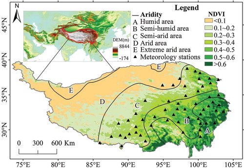
The QTP, located in western China (Figure 1), encompasses an area of approximately 2.57 × 10⁶ km² with an average elevation of approximately 4000 m above sea level (Zhang, Li, and Zheng 2002). The temperature in the southeast, with low elevations, is generally high, but it is very cold in the northwest, with higher elevations. Precipitation mainly occurs in the period from May to September, and the mean annual precipitation decreases from more than 1000–50 mm from the southeast to the northwest. These patterns of precipitation and temperature result in an increase in aridity from the southeast to the northwest (Figure 1). The QTP comprises approximately 1,521,500 km² of alpine grasslands, accounting for 59.15% of the total area (Ding et al. 2013), which includes alpine meadows, alpine steppes and alpine deserts. Regarding the growing season, the SGS mainly occurs during days 120–170, and the EGS mainly between days 250 and 300 (Ding et al. 2013). Recent studies have indicated that the grassland ecosystems of the QTP play a significant role in the ecological security of China and East Asia (Sun, Zheng, and Yao 2012).

Figure 1. Spatial pattern of aridity and NDVI in the Qinghai–Tibetan Plateau. The 57 meteorological stations used in this study are also plotted.

Dataset

NDVI, defined as the ratio of the difference between near-infrared reflectance and red visible reflectance to their sum, can effectively reflect seasonal variations in vegetation (Myneni et al. 1997; Huete et al. 2002). This index has been widely applied for monitoring interactions between climate factors and vegetation and crop growth (Son, Chen, and Chen 2012; Liu et al. 2011; Nigam et al. 2015; Kim and Yeom 2015). In this study, global inventory modeling and mapping studies (GIMMS) NDVI-3 g (NDVI, third generation) data, spanning the period from 1982 to 2012, at a spatial resolution of 8 km and at intervals of 15 d, were used, which is presently the longest NDVI dataset series. The dataset was generated by the Advanced Very High Resolution Radiometer (AVHRR) instrument onboard the National Oceanic and Atmospheric Administration (NOAA) satellite series and was provided by the Global Land Cover Facility of the University of Maryland (Tucker et al. 2005). The dataset was compiled by merging segments (data strips) of a half-month period using the Maximum Value Composition method (Holben 1986).

To investigate the relationship between the EGS and climate, we obtained daily meteorological data from 57 meteorological stations distributed across the QTP (Figure 1) and operated by the State Meteorological Administration of China (http://cdc.nmic.cn). These data, which spanned the period from 1982 to 2012, included the daily mean temperature (T_mean), daytime temperature (T_max), nighttime temperature (T_min) and precipitation data.

Determination of the ETGS

At present, there is no universal method for defining the ETGS (Linderholm 2006). In this study, we employed the definition by Linderholm, Walther, and Chen (2008) and Dong et al. (2012), namely, that ETGS is defined as the first day of the first 10-day period with a mean temperature less than 5°C.

Detection of vegetation EGS from satellite images

On the QTP, the distribution pattern of precipitation and temperature results in a progressive increase in aridity from the southeast to the northwest. In the warm and wet southeast, there is a relative small zone of evergreen forest. However, in the cold and dry west there is an extensive area with sparse or absent vegetation. In addition, Zhang et al. (2013a) have suggested that GIMMS NDVI data may suffer from severe data-quality limitations in most parts of the western plateau. Thus, to minimize the impact of bare, sparsely and evergreen vegetated regions, we used only pixels that simultaneously met the following criteria: (1) an average NDVI value during April–September of more than 0.10; (2) a maximum annual NDVI value of greater than 0.15; (3) an annual maximum NDVI value occurring between July and September; and (4) an average winter NDVI value of less than 0.4 (Shen et al. 2011; Ding et al. 2013).

Despite all the efforts to improve the data quality, the remaining atmospheric contamination in the NDVI dataset may still result in spurious variations in vegetation indices (Chen et al. 2004) and may affect the determination of the EGS. To further reduce contamination by clouds, snow, and ice, we applied a Savitzky–Golay (S–G) filtering procedure to each annual NDVI cycle (Chen et al. 2004). As a result of the S–G treatment, we obtained an initial type of processed data, comprising smoothed data with the same temporal resolution as the raw data; based on this type of data, we then obtained a further type of processed data with a temporal resolution of 1 d by spline interpolation.

A variety of methods have been developed for retrieving phenology from seasonal NDVI data (Cong et al. 2012; White et al. 2009). However, a universally accepted definition of phenological events does not exist. In the present study, we applied the “Threshold of NDVI Ratio” technique developed by White, Thornton, and Running (1997) to derive the EGS. First, based on the smoothed data with the same temporal resolution as the raw data, we determined the maximum and minimum NDVI values (Figure 2(a)). Yu, Luedeling, and Xu (2010) evaluated the average NDVI curve over 24 years (GIMMS) and noted that the NDVI reached its minimum value in February and March. To eliminate the influences of snow cover, the annual NDVI minimum was replaced by the average NDVI for these two months. Then, based on the smoothed data with a temporal resolution of 1 d, we calculated the NDVI ratio using the following formula:

(1)

where is the time. Ground observation data from 18 grassland-monitoring stations were then used to determine the appropriate threshold. The final thresholds were selected according to the mean absolute error (MAE) and the root-mean-square error (RMSE), calculated by comparing the ground observations and the modeled EGS values. Finally, we selected an NDVI ratio threshold of 0.70 (MAE = 10.14 d and RMSE = 12.52 d) for the EGS (Figure 2(b)).

Figure 2. Illustration of the NDVI ratio method used to derive the end of the growing season (EGS). (a) Some parameters used in the NDVI ratio method. (b) EGS is assumed to occur when the EGS-specific threshold is below 0.70.

Identifying EGS trends

The piecewise regression model has been widely adopted to identify trends in vegetation changes (Wang et al. 2011; Zhang et al. 2013a, 2013b). To evaluate EGS trends, we applied this model to quantitatively identify the turning points from 1982 to 2012:

(2)

where t is the year; y is the EGS; α is the estimated turning points of the EGS change trend, which was estimated by the least-squares error method; β₀, β₁ and β₂ are regression coefficients; and ϵ is the residual error. Because long time-series of EGS might contain more than one turning point, in the present work Equation (2) was modified to detect more than one turning point as follows:

(3)

where n is the number of turning points in the time-series and α_{i +1} is the time of the ith turning points. The other parameters in Equation (3) are defined as above.

To avoid linear regression in a too short period, Wang et al. (2011) confined α to within the period 1986 to 2002, whereas Che et al. (2014) analyzed the trends in the EGS by linear regression over a period of at least six years. Therefore, we confined α to within the period from 1988 to 2006 and set the minimum period between turning points to not less than six years.

Results

Change in the EGS on a regional scale

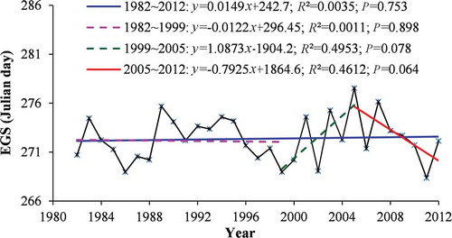
The inter-annual variations of the vegetation EGS on a regional scale from 1982 to 2012 are illustrated in Figure 3. The EGS displayed no statistically significant trend across the study period as a whole (P = 0.753); however, three different trends could be identified for the periods 1982–1999, 1999–2005, and 2005–2012. The EGS displayed no significant trend from 1982 to 1999 (P = 0.898) and then showed a delaying trend of 1.087 d year⁻¹ from 1999 to 2005 (P = 0.078); after 2005, however, the trend towards an earlier EGS appeared to be abrupt, with the onset of an advancing trend of 0.79 d year⁻¹ (P = 0.064).

Figure 3. Inter-annual variations in the end of the growing season (EGS) for the entire study area for the 1982–2012 period.

Spatial patterns of trends in the vegetation EGS

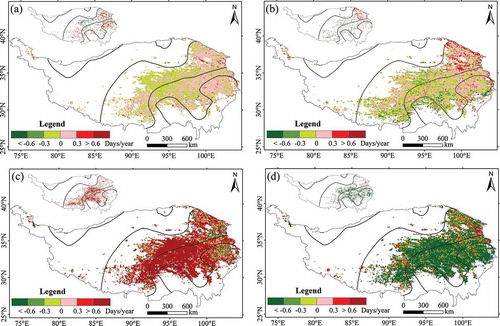
Spatial heterogeneity throughout the plateau was observed for the variation in the EGS (Figure 4). Over the entire study period (Figure 4(a) and Table 1), the pixels for which the delaying trend was significant (P < 0.1) amounted to approximately 8.18% of the total; these pixels were distributed mainly in the eastern part of the study area. Areas that showed a significant advancing trend accounted for approximately 5.24% of the total and were mainly scattered in the western part of the study area. For the period 1982–1999 (Figure 4(b) and Table 1), the pixels displaying a significant delaying trend accounted for 4.14% of the total and were mainly distributed in the east of the study area. A similar proportion of pixels displayed a significant advancing trend, and these pixels were mainly distributed in the central and western parts of the study area. For the 1999–2005 period, a clear delaying trend was evident throughout the study area; as shown in Figure 4(c) and Table 1, the proportion of pixels showing a delaying trend was 86.41%. In contrast, from 2005 to 2012 (Figure 4(d)), there was a clear advancing trend throughout the entire plateau and the proportion of pixels displaying this trend was 84.41% (Table 1). Overall, comparing the three different periods, the delaying trend for the period 1999–2005 was the most significant. However, over the study period as a whole, the trend was strongly influenced by the marked advancing trend since 2005; therefore, although the EGS displayed an overall delaying trend between 1982 and 2012, the amplitude of the change was very low.

Table 1. Percentage of pixels displaying an advancing or delaying trend in the end of the growing season (EGS).

	1982 – 2012	1982 – 1999	1999 – 2005	2005 – 2012
Advancing trend (%)	47.11	54.21	13.59	84.41
Significant advancing trend (P < 0.1) (%)	5.24	3.82	0.25	15.31
Delaying trend (%)	52.89	45.79	86.41	15.59
Significant delaying trend (P < 0.1) (%)	8.18	4.14	20.54	0.61

Figure 4. Spatial pattern of trends for the end of the growing season (EGS) throughout the study area: (a) 1982–2012, (b) 1982–1999, (c) 1999–2005, and (d) 2005–2012. The small map on top illustrates significant pixels (P < 0.1).

Correlation between the EGS and climatic factors

For the period from 1982 to 2012, the ETGS was significantly and positively correlated with the EGS across the study area (R² = 0.26, P = 0.004), and this correlation was maintained consistently throughout the plateau for the various specific zones (Figure 5). The results indicated that the ETGS influenced the vegetation EGS profoundly across the entire study area; in other words, temperature is a determinant factor for the EGS.

Figure 5. Relationship between the end of the growing season (EGS) and the end of the thermal growing season (ETGS) across meteorological stations in the entire study area (a), the humid zone (b), the semi-humid zone (c), and the semi-arid zone (d).

The correlations between the EGS and August/September temperature and precipitation for different periods and regions are shown in Table 2. For the study period overall (1982–2012), a positive correlation between the EGS and air temperature was observed during August and September, with the correlation being more apparent for September than for August. In contrast, the EGS and precipitation displayed a positive correlation for August but no relationship in September; nonetheless, the correlation in August had a low level of significance. Considering the individual periods within the overall study period, the correlation between air temperature and the EGS observed for the 1999–2005 period was more significant than that for the other periods. Regarding the spatial pattern of the correlation, the positive correlation between air temperature and the EGS diminished with the increase of aridity, whereas the positive correlation between the EGS and the amount of precipitation in August was enhanced with increasing aridity.

Table 2. Correlation between the end of the growing season (EGS) and August/September temperature and precipitation for different periods and regions.

	Period	MTmean			SP
		Aug	Sep	Aug–Sep	Aug	Sep	Aug–Sep
Humid area	1982 – 2012	0.32*	0.50***	0.49***	0.12	0.02	0.12
	1982 – 1999	0.16	0.51**	0.44*	−0.26	0.06	−0.24
	1999 – 2005	0.83**	0.73*	0.92***	0.54	0.73*	0.66
	2005 – 2012	0.00	0.26	0.28	0.54	−0.29	0.44
Semi-humid area	1982 – 2012	0.24	0.29	0.36**	0.29	−0.08	0.21
	1982 – 1999	0.12	0.47**	0.43*	−0.08	0.01	−0.06
	1999 – 2005	0.72*	0.60	0.78**	0.76*	0.32	0.75*
	2005 – 2012	0.15	−0.01	−0.42	0.69*	−0.30	0.45
Semi-arid area	1982 – 2012	0.08	0.28	0.19	0.27	−0.07	0.24
	1982 – 1999	−0.34	0.42*	0.13	0.17	−0.02	0.21
	1999 – 2005	0.77**	0.78**	0.85**	0.43	0.09	0.31
	2005 – 2012	0.29	−0.07	0.21	0.70*	−0.16	0.45

Note: MT_mean: mean of daily mean temperature; SP: sum of precipitation; ***P < 0.01; **P < 0.05; *P < 0.1.

There was a positive correlation between the EGS and the daily mean temperature for each of the pre-senescence periods (15, 30 and 60 d) (Table 3). However, this correlation was significantly reduced with the increase of aridity. In the semi-humid and semi-arid zones, this positive correlation was also significantly reduced as the length of the pre-senescence period extended. In this study, we also evaluated the effects of daytime temperature (T_max) or nighttime temperature (T_min) during pre-senescence periods on the EGS (Table 4). During the entire study period (1982–2012), there was also a positive correlation between the EGS and T_max or T_min for each of the pre-senescence periods (15, 30 and 60 d). With the increase of aridity, the correlation coefficient showed a reducing trend, similar to daily mean temperature. Additionally, we found a difference in the response of the EGS to T_max and T_min, such that the correlation coefficient between the EGS and T_max decreased and that between the EGS and T_min increased with the lengthening of the EGS. Regarding precipitation (Table 3), the correlation with the EGS was very complex for the different pre-senescence periods. In the humid area, it was found that the shorter the period before the onset of the EGS, the more noticeable was the influence of precipitation upon the EGS. However, with the increase of aridity, precipitation showed increasing importance with regard to the length of the EGS extension. Considering the individual periods within the overall study period, the correlations between the EGS and pre-senescence temperature and the amount of pre-senescence precipitation observed for the 1999–2005 period were more significant than those for any of the other periods. The results indicated that climate factors profoundly influenced the vegetation EGS across the entire study area from 1999 to 2005.

Table 3. Correlation between the end of the growing season (EGS) and mean temperature and cumulative precipitation prior to EGS for different periods and regions.

Study area	Period	MTmean for 15 d period before EGS	MTmean for 30 d period before EGS	MTmean for 60 d period before EGS	SP for 15 d period before EGS	SP for 30 d period before EGS	SP for 60 d period before EGS
Humid area	1982 – 2012	0.45**	0.52***	0.51***	0.22	0.03	0.15
	1982 – 1999	0.20	0.44*	0.47*	0.40*	0.21	−0.23
	1999 – 2005	0.92***	0.72**	0.92***	0.56	0.63	0.66
	2005 – 2012	0.61	0.53	0.43	0.02	−0.36	0.45
Semi-humid area	1982 – 2012	0.47***	0.40**	0.36**	−0.04	−0.06	0.25
	1982 – 1999	0.43*	0.49**	0.44*	0.26	0.07	−0.02
	1999 – 2005	0.89***	0.66	0.80*	0.45	0.42	0.78**
	2005 – 2012	0.47	0.09	0.11	−0.37	−0.42	0.49
Semi-acid area	1982 – 2012	0.33*	0.23	0.14	−0.03	0.10	0.27
	1982 – 1999	0.40	0.35	0.10	0.32	0.12	0.20
	1999 – 2005	0.81**	0.79**	0.84**	0.25	0.13	0.26
	2005 – 2012	0.13	−0.11	0.05	−0.53	0.08	0.57

Note: MT_mean: mean of daily mean temperature; SP: sum of precipitation; ***P < 0.01; **P < 0.05; *P < 0.1.

Table 4. Correlation between the end of the growing season (EGS) and mean daytime temperature (T_max) and night-time temperature (T_min) prior to the EGS for different periods and regions.

Study area	Period	MTmin for 15 d period before EGS	MTmin for 30 d period before EGS	MTmin for 60 d period before EGS	MTmax for 15 d period before EGS	MTmax for 30 d period before EGS	MTmax for 60 d period before EGS
Humid area	1982 – 2012	0.36**	0.48***	0.48***	0.45**	0.45**	0.4**
	1982 –1999	0.15	0.45*	0.20	0.20	0.33	0.51**
	1999 – 2005	0.95***	0.82**	0.95***	0.66	0.49	0.60
	2005 – 2012	0.13	0.15	0.80**	0.65*	0.70*	−0.10
Semi-humid area	1982 – 2012	0.35*	0.34*	0.42**	0.47***	0.35*	0.23
	1982 – 1999	0.49**	0.43*	0.30	0.33	0.41*	0.42*
	1999 – 2005	0.91***	0.86**	0.91***	0.68*	0.39	0.34
	2005 – 2012	−0.07	−0.15	0.70*	0.64*	0.28	−0.19
Semi-acid area	1982 – 2012	0.24	0.18	0.20	0.33*	0.23	0.02
	1982 – 1999	0.45*	0.33	0.18	0.36	0.40	−0.01
	1999 – 2005	0.84**	0.74*	0.92***	0.69*	0.65	0.68*
	2005 – 2012	−0.17	−0.11	0.37	0.19	−0.32	−0.27

Note: MT_min: mean of night-time temperature (T_min); MT_max: mean of daytime temperature (T_max); ***P < 0.01; **P < 0.05; *P < 0.1.

Discussion

Changes in the EGS based on meta-analysis

As shown in Figure 6, there was a high level of consistency in the trend in the inter-annual variation in the EGS between the retrieved EGS results based on GIMMS-3 g and those based on SPOT VGT (R = 0.603, P = 0.022). Furthermore, the accuracy of the retrieved EGS results in this study was also assessed by comparison with the findings of previous studies (Che et al. 2014; Ding et al. 2013; Yu, Luedeling, and Xu 2010). At the regional scale, the trend in the annual changes in the EGS for the period 1982–2007 is in agreement with the results of Che et al. (2014), who used GIMMS-3 g LAI to derive the EGS on the QTP. Similarly, the trend for the 1999–2009 period is in accordance with the findings of Ding et al. (2013). Admittedly, this qualitative examination of derived EGS values is less accurate than quantitative analyses; however, it is the only method available when observational data are lacking (Che et al. 2014).

Figure 6. Comparison of inter-annual variation in the end of the growing season (EGS) derived from SPOT and GIMMS-3 g for the period 1999–2012. The correlation coefficient R- and its P-value between the two datasets are shown in the figure.

Temperature thresholds for the EGS

The relationship between the temperature or the accumulative temperature on the date of the EGS and the mean annual temperature across all the meteorological stations (Figure 7) illustrates that both the temperature threshold and the accumulative temperature threshold for the EGS were significantly and positively correlated with the mean annual temperature (P < 0.001). The results indicate that the vegetation growing season ended at a lower temperature in colder locations than in warmer areas. This suggests that, with a trend towards global warming, the vegetation growing season may occur at higher temperatures and that the threshold temperature (the temperature on the date of the EGS) required to trigger the EGS may therefore also be higher. Such an increase in the EGS threshold in response to a rising mean annual temperature could likely be attributed to growth acclimation to higher temperatures (Piao et al. 2011; White, Running, and Thornton 1999). The observed dependence of the EGS on the mean annual temperature suggests that, on the QTP, a 1°C increase in the mean annual temperature would increase the temperature threshold for the vegetation EGS by 0.75°C; this is in good agreement with the results of Piao et al. (2011) and Jin et al. (2013). We also found that the temperature thresholds for EGS have no universal definition. Most of the thresholds in this study were higher than 2°C (92.81.%), which was in approximate agreement with the findings of Jin et al. (2013). However, the conclusions above are inferred only from remote sensing data and meteorological data; additional in situ observational data of vegetation phenology and further research will be required to determine whether the results predict that the EGS at any given location will respond to an increased temperature or to an increased cumulative temperature as the climate becomes warmer.

Figure 7. Relationship between the temperature threshold of the end of the growing season (EGS) and the mean annual temperature for meteorological stations across the Qinghai–Tibetan Plateau. (a) Temperature threshold. (b) Accumulative temperature threshold.

The spatial heterogeneity of the correlation between the EGS and climate factors

Our analysis indicated a clear positive response of the EGS to temperature across the study area, which was consistent with the results from previous studies (Che et al. 2014; Jin et al. 2013). In general, for the entire study period, the EGS was most significantly correlated with the ETGS. However, the correlation between the EGS and air temperature exhibited divergence across the study area; the importance of air temperature gradually decreased with the increase of aridity. Compared to the effects of air temperature, the impact of precipitation on the EGS is extremely complex.

Based on the results of our study, it is clear that the EGS shows a more significant correlation with the air temperature in September than with the air temperature in August (Table 2). On the QTP, the highest monthly air temperatures occur from June to August; the vegetation grows rapidly during this period, and the NDVI reaches its peak in August. Therefore, the air temperature during this phase has a weak effect on the EGS (Che et al. 2014). The air temperature, however, begins to decline in September. Because the temperature-related senescence of vegetation is mainly modulated by cumulative cold temperatures below a specific threshold (Jeong et al. 2011), warmer air temperatures in September can result in a delay in the EGS.

Regarding precipitation, the precipitation in the southeast of QTP is adequate for the growth of vegetation; therefore, the impact of precipitation is very low. However, in the semi-humid or semi-arid zones of the north-west of the QTP, the impact of precipitation on the EGS is much greater (Che et al. 2014). As also noted by Zhou, Yang, and Fang (2007), the distribution of vegetation in this north-western area is mainly influenced by precipitation. However, we found that the EGS showed a positive correlation with precipitation in August but no relationship with precipitation in September. This may be because the EGS date in this area was found to occur mainly in early September and the increase in precipitation in September resulted in an air temperature decrease.

The pre-senescence temperature plays a more significant role than pre-senescence precipitation in shaping the spatial pattern of the trend in the EGS (Tables 3 and 4). Across the study area, the EGS was positively correlated with the pre-senescence mean temperature for the entire study period. However, the correlation was gradually reduced with the increase of aridity. Jin et al. (2013) reported that soil wetting is an important regulator of the response of the vegetation EGS to temperature change. In our study, the correlation was also for the different lengths of the pre-senescence period. In the humid zone, the pre-senescence temperature always showed an important influence on the EGS. However, in the semi-humid and semi-arid zones, the correlation was gradually reduced for the daily maximum temperature and enhanced for the daily mean and minimum temperature with extension of the length of the pre-senescence period. Piao et al. (2015) found the vegetation green-up in spring is triggered more by the daytime temperature (T_max) than by the night-time temperature (T_min). However, our study found no significant difference between the response of the EGS to T_max and T_min. Regarding precipitation, a distinct difference in effects was observed between the humid zone and the semi-humid and semi-arid zones. In the humid zone, the influence of precipitation increased as the pre-senescence period under consideration became shorter (i.e., as the length of time prior to the EGS decreased). In contrast, the opposite relationship was observed for the semi-humid and semi-arid zones, in which the summer season is very short; precipitation likely leads to a decline in air temperature when it occurs close to the date of the EGS, and this leads to a reduction in the impact of precipitation.

Numerous studies have been conducted on the relationships between phenology and climatic factors on the QTP (Zhang et al. 2013a; Yu, Luedeling, and Xu 2010; Shen et al. 2011; Piao et al. 2011); however, there are few reports on the impact of climatic factors on autumn phenology (Che et al. 2014; Yu, Luedeling, and Xu 2010; Jin et al. 2013). Autumn phenology is a more complicated process than spring phenology (Chmielewski and Rotzer 2001), and achieving an adequate understanding of its long-term variations is very difficult (Jeong et al. 2011). In the present study, only climatic factors, such as air temperature, precipitation, soil moisture and temperature, and sunlight duration, were used to assess the response of the EGS to climate change. However, variations in the EGS may also be affected by other factors, such as grassland degradation (Che et al. 2014; Chen et al. 2011) and human activities (Shen et al. 2011); therefore, the influence of these factors should be clarified in the future.

Conclusions

In this study, based on the satellite-derived NDVI and meteorological record from 1982 to 2012, we analyzed the spatial patterns of variations in the vegetation EGS and their relationships with temperature and precipitation on the QTP. The following conclusions were drawn:

1. There is a high level of consistency in the trend between the retrieved EGS results from the GIMMS-3 g and SPOT VGT (R = 0.603, P = 0.022). We also used the findings of previous studies to assess the accuracy of the retrieved EGS results in this study and found that there was also a good consistency in the trend.

2. For the whole study period (1982–2012), the EGS displayed no statistically significant trend at the regional scale (P = 0.753). However, within this overall period, three different trends were apparent. From 1982 to 1999, the EGS displayed no significant trend (P = 0.898); from 1999 to 2005, it displayed a delaying trend of 1.087 d year⁻¹ (P = 0.078); and finally, after 2005, there was a clear advancing trend.

3. Clear spatial heterogeneity was observed throughout the plateau for the three different periods. Those areas showing a delaying trend were mainly distributed in the eastern part of the QTP, whereas those showing an advancing trend were mostly scattered in the west.

4. Throughout the study period, the ETGS was significantly and positively correlated with the EGS (P = 0.004), and this correlation was consistent throughout the plateau for the various areas.

5. An analysis of the correlation between the EGS and climate factors indicated a clear positive response of the EGS to temperature across the study area. In addition, the change in the vegetation EGS was more closely correlated with air temperature than with precipitation. However, the importance of temperature gradually decreased with the increase of aridity. The pre-senescence temperature plays a more significant role than pre-senescence precipitation in shaping the spatial patterns of the trend in the EGS, yet this significance also became lower as the aridity increased. These results suggest that precipitation is an important regulator of the response of the vegetation EGS to climate warming, and also indicate that spatial difference is the key environmental influence on the vegetation EGS.

Disclosure statement

No potential conflict of interest was reported by the authors.

Additional information

Funding

This work was supported by the Strategic Priority Research Program of the Chinese Academy of Sciences [grant number XDB03030500]; National Natural Science Foundation of China [grant number 41201095], [grant number 41171080], [grant number 41371120], and [grant number 41201055].

References

- Badeck, F. W., A. Bondeau, K. Bottcher, D. Doktor, W. Lucht, J. Schaber, and S. Sitch. 2004. “Responses of Spring Phenology to Climate Change.” New Phytologist 162 (2): 295–309. doi:10.1111/j.1469-8137.2004.01059.x.
- Both, C., S. Bouwhuis, C. M. Lessells, and M. E. Visser. 2006. “Climate Change and Population Declines in a Long-Distance Migratory Bird.” Nature 441 (7089): 81–83. doi:10.1038/nature04539.
- Che, M. L., B. Z. Chen, J. L. Innes, G. Y. Wang, X. M. Dou, T. M. Zhou, H. F. Zhang, J. W. Yan, G. Xu, and H. W. Zhao. 2014. “Spatial and Temporal Variations in the End Date of the Vegetation Growing Season Throughout the Qinghai-Tibetan Plateau from 1982 to 2011.” Agricultural and Forest Meteorology 189: 81–90. doi:10.1016/j.agrformet.2014.01.004.
- Chen, H., Q. A. Zhu, N. Wu, Y. F. Wang, and C.-H. Peng. 2011. “Delayed Spring Phenology on the Tibetan Plateau May Also Be Attributable to Other Factors Than Winter and Spring Warming.” Proceedings of the National Academy of Sciences of the United States of America 108 (19): E93–E93. doi:10.1073/pnas.1100091108.
- Chen, J., P. Jonsson, M. Tamura, Z. H. Gu, B. Matsushita, and L. Eklundh. 2004. “A Simple Method for Reconstructing A High-Quality NDVI Time-Series Data Set Based on the Savitzky-Golay Filter.” Remote Sensing of Environment 91 (3–4): 332–344. doi:10.1016/j.rse.2004.03.014.
- Chmielewski, F. M., and T. Rotzer. 2001. “Response of Tree Phenology to Climate Change across Europe.” Agricultural and Forest Meteorology 108 (2): 101–112. doi:10.1016/s0168-1923(01)00233-7.
- Churkina, G., D. Schimel, B. H. Braswell, and X. M. Xiao. 2005. “Spatial Analysis of Growing Season Length Control over Net Ecosystem Exchange.” Global Change Biology 11 (10): 1777–1787. doi:10.1111/j.1365-2486.2005.001012.x.
- Cleland, E. E., N. R. Chiariello, S. R. Loarie, H. A. Mooney, and C. B. Field. 2006. “Diverse Responses of Phenology to Global Changes in a Grassland Ecosystem.” Proceedings of the National Academy of Sciences of the United States of America 103 (37): 13740–13744. doi:10.1073/pnas.0600815103.
- Cong, N., S. L. Piao, A. P. Chen, X. H. Wang, X. Lin, S. P. Chen, S. J. Han, G. S. Zhou, and X. P. Zhang. 2012. “Spring Vegetation Green-Up Date in China Inferred from SPOT NDVI Data: A Multiple Model Analysis.” Agricultural and Forest Meteorology 165: 104–113. doi:10.1016/j.agrformet.2012.06.009.
- Dai, J. H., H. J. Wang, and Q. S. Ge. 2013. “Multiple Phenological Responses to Climate Change among 42 Plant Species in Xi’an, China.” International Journal of Biometeorology 57 (5): 749–758. doi:10.1007/s00484-012-0602-2.
- Dai, J. H., H. J. Wang, and Q. S. Ge. 2014. “The Spatial Pattern of Leaf Phenology and Its Response to Climate Change in China.” International Journal of Biometeorology 58 (4): 521–528. doi:10.1007/s00484-013-0679-2.
- Ding, M. J., Y. L. Zhang, L. S. Liu, W. Zhang, Z. F. Wang, and W. Q. Bai. 2007. “The Relationship between NDVI and Precipitation on the Tibetan Plateau.” Journal of Geographical Sciences 17 (3): 259–268. doi:10.1007/s11442-007-0259-7.
- Ding, M. J., Y. L. Zhang, X. M. Sun, L. S. Liu, Z. F. Wang, and W. Q. Bai. 2013. “Spatiotemporal Variation in Alpine Grassland Phenology in the Qinghai-Tibetan Plateau from 1999 to 2009.” Chinese Science Bulletin 58 (3): 396–405. doi:10.1007/s11434-012-5407-5.
- Dong, M. Y., Y. Jiang, C. T. Zheng, and D. Y. Zhang. 2012. “Trends in the Thermal Growing Season Throughout the Tibetan Plateau during 1960-2009.” Agricultural and Forest Meteorology 166: 201–206. doi:10.1016/j.agrformet.2012.07.013.
- Fu, Y., H. C. Zhang, W. J. Dong, and W. P. Yuan. 2014. “Comparison of Phenology Models for Predicting the Onset of Growing Season over the Northern Hemisphere.” PlOS ONE 9 (10): e109544–e109544. doi:10.1371/journal.pone.0109544.
- Holben, B. N. 1986. “Characteristics of Maximum-Value Composite Images from Temporal AVHRR Data.” International Journal of Remote Sensing 7 (11): 1417–1434. doi:10.1080/01431168608948945.
- Huete, A., K. Didan, T. Miura, E. P. Rodriguez, X. Gao, and L. G. Ferreira. 2002. “Overview of the Radiometric and Biophysical Performance of the MODIS Vegetation Indices.” Remote Sensing of Environment 83 (1–2): 195–213. doi:10.1016/s0034-4257(02)00096-2.
- IPCC. 2013. Climate Change 2013: The Physical Science Basis. Contribution of Working Group I to the Fifth Assessment Report of the Intergovernmental Panel on Climate Change, 5–8. Cambridge: Cambridge University Press.
- Jeong, S.-J., C.-H. Ho, H.-J. Gim, and M. E. Brown. 2011. “Phenology Shifts at Start Vs. End of Growing Season in Temperate Vegetation over the Northern Hemisphere for the Period 1982-2008.” Global Change Biology 17 (7): 2385–2399. doi:10.1111/j.1365-2486.2011.02397.x.
- Jin, Z. N., Q. L. Zhuang, J.-S. He, T. X. Luo, and Y. Shi. 2013. “Phenology Shift from 1989 to 2008 on the Tibetan Plateau: An Analysis with a Process-Based Soil Physical Model and Remote Sensing Data.” Climatic Change 119 (2): 435–449. doi:10.1007/s10584-013-0722-7.
- Kim, H.-O., and J.-M. Yeom. 2015. “Sensitivity of Vegetation Indices to Spatial Degradation of Rapideye Imagery for Paddy Rice Detection: A Case Study of South Korea.” GIScience & Remote Sensing 52 (1): 1–17. doi:10.1080/15481603.2014.1001666.
- Linderholm, H. W. 2006. “Growing Season Changes in the Last Century.” Agricultural and Forest Meteorology 137 (1–2): 1–14. doi:10.1016/j.agrformet.2006.03.006.
- Linderholm, H. W., A. Walther, and D. L. Chen. 2008. “Twentieth-Century Trends in the Thermal Growing Season in the Greater Baltic Area.” Climatic Change 87 (3–4): 405–419. doi:10.1007/s10584-007-9327-3.
- Liu, Y., X. F. Wang, M. Guo, H. Tani, N. Matsuoka, and S. Matsumura. 2011. “Spatial and Temporal Relationships among NDVI, Climate Factors, and Land Cover Changes in Northeast Asia from 1982 to 2009.” GIScience & Remote Sensing 48 (3): 371–393. doi:10.2747/1548-1603.48.3.371.
- Memmott, J., P. G. Craze, N. M. Waser, and M. V. Price. 2007. “Global Warming and the Disruption of Plant-Pollinator Interactions.” Ecology Letters 10 (8): 710–717. doi:10.1111/j.1461-0248.2007.01061.x.
- Meroni, M., M. M. Verstraete, F. Rembold, F. Urbano, and F. Kayitakire. 2014. “A Phenology-Based Method to Derive Biomass Production Anomalies for Food Security Monitoring in the Horn of Africa.” International Journal of Remote Sensing 35 (7): 2472–2492. doi:10.1080/01431161.2014.883090.
- Myneni, R. B., C. D. Keeling, C. J. Tucker, G. Asrar, and R. R. Nemani. 1997. “Increased Plant Growth in the Northern High Latitudes from 1981 to 1991.” Nature 386 (6626): 698–702. doi:10.1038/386698a0.
- Nigam, R., S. S. Vyas, B. K. Bhattacharya, M. P. Oza, S. S. Srivastava, N. Bhagia, D. Dhar, and K. R. Manjunath. 2015. “Modeling Temporal Growth Profile of Vegetation Index from Indian Geostationary Satellite for Assessing In-Season Progress of Crop Area.” GIScience & Remote Sensing 52 (6):723–745. doi:10.1080/15481603.2015.1073036.
- Parmesan, C., and G. Yohe. 2003. “A Globally Coherent Fingerprint of Climate Change Impacts across Natural Systems.” Nature 421 (6918): 37–42. doi:10.1038/natu-re01286.
- Penuelas, J., I. Filella, X. Y. Zhang, L. Llorens, R. Ogaya, F. Lloret, P. Comas, M. Estiarte, and J. Terradas. 2004. “Complex Spatiotemporal Phenological Shifts as a Response to Rainfall Changes.” New Phytologist 161 (3): 837–846. doi:10.1111/j.1469-8137.2004.01003.x.
- Penuelas, J., T. Rutishauser, and I. Filella. 2009. “Phenology Feedbacks on Climate Change.” Science 324 (5929): 887–888. doi:10.1126/science.1173004.
- Piao, S. L., M. D. Cui, A. P. Chen, X. H. Wang, P. Ciais, J. Liu, and Y. H. Tang. 2011. “Altitude and Temperature Dependence of Change in the Spring Vegetation Green-Up Date from 1982 to 2006 in the Qinghai-Xizang Plateau.” Agricultural and Forest Meteorology 151 (12): 1599–1608. doi:10.1016/j.agrformet.2011.06.016.
- Piao, S. L., J. Y. Fang, W. Ji, Q. H. Guo, J. H. Ke, and S. Tao. 2004. “Variation in a Satellite-Based Vegetation Index in Relation to Climate in China.” Journal of Vegetation Science 15 (2): 219–226. doi:10.1658/1100-9233(2004)015[0219:viasvi]2.0.co;2.
- Piao, S. L., P. Friedlingstein, P. Ciais, N. Viovy, and J. Demarty. 2007. “Growing Season Extension and Its Impact on Terrestrial Carbon Cycle in the Northern Hemisphere over the past 2 Decades.” Global Biogeochemical Cycles 21: 3. doi:10.1029/2006gb002888.
- Piao, S. L., J. G. Tan, A. P. Chen, Y. S. H. Fu, P. Ciais, Q. Liu, and I. A. Janssens. et al. 2015. “Leaf Onset in the Northern Hemisphere Triggered by Daytime Temperature.” Nature Communications 6. doi:10.1038/ncomms7911.
- Schwartz, M. D., and J. M. Hanes. 2010. “Intercomparing Multiple Measures of the Onset of Spring in Eastern North America.” International Journal of Climatology 30 (11): 1614–1626. doi:10.1002/joc.2008.
- Shen, M. G., Y. H. Tang, J. Chen, X. L. Zhu, and Y. H. Zheng. 2011. “Influences of Temperature and Precipitation before the Growing Season on Spring Phenology in Grasslands of the Central and Eastern Qinghai-Tibetan Plateau.” Agricultural and Forest Meteorology 151 (12): 1711–1722. doi:10.1016/j.agrformet.2011.07.003.
- Sherry, R. A., X. H. Zhou, S. L. Gu, J. A. Arnone, D. S. Schimel, P. S. Verburg, L. L. Wallace, and Y. Q. Luo. 2007. “Divergence of Reproductive Phenology Under Climate Warming.” Proceedings of the National Academy of Sciences of the United States of America 104 (1): 198–202. doi:10.1073/pnas.0605642104.
- Son, N. T., C. R. Chen, and C. F. Chen. 2012. “Investigating Rice Cropping Practices and Growing Areas from MODIS Data Using Empirical Mode Decomposition and Support Vector Machines.” GIScience & Remote Sensing 49 (1): 117–138. doi:10.2747/1548-1603.49.1.117.
- Song, Y. L., H. W. Linderholm, D. L. Chen, and A. Walther. 2010. “Trends of the Thermal Growing Season in China, 1951-2007.” International Journal of Climatology 30 (1): 33–43. doi:10.1002/joc.1868.
- Sun, H. L., D. Zheng, and T. D. Yao. 2012. “Protection and Construction of the National Ecological Security Shelter Zone on Tibetan Plateau.” Acta Geographica Sinica 67 (1): 3–12. doi:10.11821/xb201201001.
- Tang, Y. H., S. Q. Wan, J. S. He, and X. Q. Zhao. 2009. “Foreword to the Special Issue: Looking into the Impacts of Global Warming from the Roof of the World.” Journal of Plant Ecology 2 (4): 169–171. doi:10.1093/jpe/rtp026.
- Tucker, C. J., J. E. Pinzon, M. E. Brown, D. A. Slayback, E. W. Pak, R. Mahoney, E. F. Vermote, and N. E. Saleous. 2005. “An Extended AVHRR 8-Km NDVI Dataset Compatible with MODIS and SPOT Vegetation NDVI Data.” International Journal of Remote Sensing 26 (20): 4485–4498. doi:10.1080/01431160500168686.
- Wang, X. H., S. L. Piao, P. Ciais, J. S. Li, P. Friedlingstein, C. Koven, and A. P. Chen. 2011. “Spring Temperature Change and Its Implication in the Change of Vegetation Growth in North America from 1982 to 2006.” Proceedings of the National Academy of Sciences of the United States of America 108 (4): 1240–1245. doi:10.1073/pnas.1014425108.
- White, M. A., K. M. Beurs, K. Didan, D. W. Inouye, A. D. Richardson, O. P. Jensen, and J. O’Keefe, et al. 2009. “Intercomparison, Interpretation, and Assessment of Spring Phenology in North America Estimated from Remote Sensing for 1982-2006.” Global Change Biology 15 (10): 2335–2359. doi:10.1111/j.1365-2486.2009.01910.x.
- White, M. A., S. W. Running, and P. E. Thornton. 1999. “The Impact of Growing-Season Length Variability on Carbon Assimilation and Evapotranspiration over 88 Years in the Eastern US Deciduous Forest.” International Journal of Biometeorology 42: 139–145. doi:10.1007/s004840050097.
- White, M. A., P. E. Thornton, and S. W. Running. 1997. “A Continental Phenology Model for Monitoring Vegetation Responses to Interannual Climatic Variability.” Global Biogeochemical Cycles 11 (2): 217–234. doi:10.1029/97gb00330.
- Yu, H. Y., E. Luedeling, and J. C. Xu. 2010. “Winter and Spring Warming Result in Delayed Spring Phenology on the Tibetan Plateau.” Proceedings of the National Academy of Sciences of the United States of America 107 (51): 22151–22156. doi:10.1073/pnas.1012490107.
- Yuan, F., C. Z. Wang, and M. Mitchell. 2014. “Spatial Patterns of Land Surface Phenology Relative to Monthly Climate Variations: US Great Plains.” GIScience & Remote Sensing 51 (1): 30–50. doi:10.1080/15481603.2014.883210.
- Zhang, G. L., Y. J. Zhang, J. W. Dong, and X. M. Xiao. 2013a. “Green-Up Dates in the Tibetan Plateau Have Continuously Advanced from 1982 to 2011.” Proceedings of the National Academy of Sciences of the United States of America 110 (11): 4309–4314. doi:10.1073/pnas.1210423110.
- Zhang, Y. L., J. G. Gao, L. S. Liu, Z. F. Wang, M. J. Ding, and X. C. Yang. 2013b. “Ndvi-Based Vegetation Changes and Their Responses to Climate Change from 1982 to 2011: A Case Study in the Koshi River Basin in the Middle Himalayas.” Global and Planetary Change 108: 139–148. doi:10.1016/j.gloplacha.2013.06.012.
- Zhang, Y. L., B. Y. Li, and D. Zheng. 2002. “A Discussion on the Boundary and Area of the Tibetan Plateau in China.” Geographical Research 21 (1): 1–8. doi:10.3321/j.issn:1000-0585.2002.01.001.
- Zhou, R., Y. H. Yang, and J. Y. Fang. 2007. “Responses of Vegetation Activity to Precipitation Variation on the Tibetan Plateau.” Acta Scientiarum Naturalium Universitatis Pekinensis 43 (6): 771–775. doi:10.3321/j.issn:0479-8023.2007.06.007.