Estimation of hourly and daily evapotranspiration and soil moisture using downscaled LST over various urban surfaces

Abstract

Surface moisture is important to link land surface temperature (LST) to people’s thermal comfort. In urban areas, the surface roughness from buildings and urban trees impacts wind speed, and consequently surface moisture. To find the role of surface roughness in surface moisture estimation, we developed methods to estimate daily and hourly evapotranspiration (ET) and soil moisture, based on a case study of Indianapolis, Indiana, USA. In order to capture the spatial and temporal variations of LST, hourly and daily LST was produced by downscaling techniques. Given the heterogeneity in urban areas, fractions of vegetation, soil, and impervious surfaces were calculated. To describe the urban morphology, surface roughness parameters were calculated from digital elevation model (DEM), digital surface model (DSM), and Terrestrial Light Detection and Ranging (LiDAR). Two source energy balance (TSEB) model was employed to generate ET, and the temperature vegetation index (TVX) method was used to calculate soil moisture. Stable hourly soil moisture fluctuated from 15% to 20%, and daily soil moisture increased due to precipitation and decreased due to seasonal temperature change. ET over soil, vegetation, and impervious surface in the urban areas yielded different patterns in response to precipitation. The surface roughness from high-rise has bigger influence on ET in central urban areas.

Keywords:

• Evapotranspiration (ET)
• soil moisture
• urban
• downscaling LST
• roughness length
• displacement height

1. Introduction

The knowledge of surface moisture in urban areas is significant because it is one of the important factors that links land surface temperature (LST) to air temperature (Carlson and Arthur 2000). A combination of air temperature, wind speed, humidity, and short and longwave radiation exposure determines a person’s thermal comfort during urban heat island effects and heat waves (Voogt and Oke 2003). The study of urban surface moisture faces one of the greatest challenges in urban remote sensing because currently available models and methods to estimate surface moisture were mainly developed for forest and agricultural areas, and empirical values or functions to compute the values of roughness conditions were set up according to vegetation types, e.g., forest, grass, and crops, in those models (Kato and Yamaguchi 2007; Weng et al. 2013). However, in urban areas, the morphology, formed by buildings, urban trees, and other surface covers, varies from place to place. Therefore, how to apply those models and methods developed for natural settings to urban areas is a scientific question that must be addressed.

LST is an essential variable in the estimation of evapotranspiration (ET) and surface moisture. Derivation of LST data from remotely sensed imagery has become more mature (Weng 2009). Compared to air temperature measured by weather stations, LSTs derived from satellite images have great advantages in flexible combinations of spatial and temporal resolutions. For example, LSTs from the Landsat family have a combination of 60–120 m spatial resolution and 16 days temporal resolution; LSTs from moderate-resolution imaging spectroradiometer (MODIS) have a 1-km spatial resolution and 1-day temporal resolution; and LSTs from Geostationary satellites (e.g., GOES) have 4-km spatial resolution and 15-min temporal resolution. In addition to the various spatial and temporal resolutions from the thermal infrared sensors, thermal downscaling techniques have the potential to increase the spatial and temporal resolutions even more (Agam et al. 2007; Inamdar and French 2009; Yang et al. 2011; Zakšek and Oštir 2012). For instance, the downscaled Landsat LSTs could have 30-m resolution in a daily interval (Weng, Fu., and Gao 2014), and downscaled GOES images could have 1-km resolution every 15 min (Weng and Fu 2014).

Given the recent advances in LST data and downscaling techniques, studies on the relationship between LST and air temperature become highly desirable. The two most important links between LST and air temperature are vegetation cover and surface moisture (Carlson and Arthur 2000). Although the relationship between temperature and vegetation cover has been intensively studied (Weng 2009), few efforts have been made on the estimation of surface moisture in urban areas (Ramamurthy and Bou-Zeid 2014).

The primary objective of this paper is to assess the surface moisture in urban areas, or more specifically, on vegetation, soil, and impervious surfaces, respectively, and to identify the impact of urban morphology from buildings and trees on surface moisture.

2. Background

2.1. ET over various urban surfaces

The surface moisture on vegetation cover, impervious surfaces, and soil can be measured by vegetation transpiration, evaporation over impervious surfaces, and soil moisture. ET is the sum of evaporation and plant transpiration. Transpiration is the process in which water is absorbed by plants’ roots and is moved to pores on the underside of leaves, where it changes to vapor and is released to the atmosphere. It is controlled by several atmospheric factors: temperature, relative humidity, topographic condition, wind and air movement, and soil moisture availability (Penman and Long 1960; Monteith 1965; Christensen, Tague, and Baron 2008; Strelcova et al. 2013). In agricultural and forest areas, the studies on transpiration usually were conducted on individual or several species (Strelcova et al. 2013). However, in urban areas, urban forests and street trees contain a diverse mix of species from many regions worldwide. Therefore, the studies of transpiration in urban areas specifically considered the diversity of the species and hypothesized that species played a more important role than meteorological variables (Pataki et al. 2011). Urban built environments increase urban runoff and slow down the infiltration rate, which reduces the transpiration rate and limits the rooting depth of urban trees (Bartens et al. 2009). Plant density varies in urban areas as well. Hagishima, Narita, and Tanimoto (2007) suggested that the small size plants and low spatial density vegetation may result in an increase in ET and latent heat flux in urban areas. The land cover of urban surfaces impacts urban tree transpiration because energy fluxes and ambient humidity may impact the leaf-to-air vapor pressure, consequently, prolonging or shortening the stomatal closure (Kjelgren and Montague 1998).

Evaporation over impervious surfaces is one of the least studied topics in the fields of urban hydrology and microclimatology (Ramamurthy and Bou-Zeid 2014). Urban areas play an important role in global climate change because of the urban heat island effects, heat wave hazards, and urban runoff. To measure the impact of urban climate in regional or global scale models, one of the areas that have not been thoroughly studied is urban surface moisture. Impervious surfaces contribute to urban evaporation (Ramamurthy and Bou-Zeid 2014); urban evaporation greatly impacts air temperature, which is what people suffer from the extreme weather conditions. With the LST derived from satellite images in various combinations of temporal and spatial resolution, and the maturity of the techniques of surface temperature derivation, LST becomes more and more popular to heat-related hazard monitoring. Therefore, methods to link LST and air temperature are a way of monitoring heat-related hazards in the future.

In urban areas, the land surface can be depicted by three major components: vegetation cover, impervious surfaces, and soil (Ridd 1995; Weng and Lu 2009). In remote sensing, the land cover surface in each pixel can be described by the percentage of vegetation cover, impervious surfaces, and soil. Figure 1 shows the vegetation–impervious surface–soil (VIS) model, which illustrates the features of an urban landscape.

Figure 1. The illustration of urban and near urban features and the characteristics of an urban landscape in the vegetation–impervious surface–soil (VIS) model (Ridd 1995). For full color versions of the figures in this paper, please see the online version.

2.2. Soil moisture

Soil moisture is water held in the pore spaces of soil. The volumetric soil moisture is the ratio of the volume of water and the volume of soil, water, and air (Rahimzadeh-Bajgiran et al. 2013). The public is aware of the problems of water storage and soil erosion in rural areas and the importance of soil moisture management to secure food production and water supply (Shaxson and Barber 2003). When the soil is less porous, surface runoff increases. As a result, rainfall cannot support plant growth and sustain surface water levels (Shaxson and Barber 2003). In urban areas, research on soil moisture focused on the influence on the urban microclimate and surface layer meteorology. The relationship between soil moisture, temperature, and wind speed has been studied by Husain, Bélair, and Leroyer (2014). They found that high soil moisture was associated with colder near-surface temperature and lower near-surface wind speed, while lower soil moisture was associated with warmer near-surface temperature and higher near-surface wind speed. Compared to soil moisture condition in rural areas, urban soil moisture content was predicted to have smaller impacts on surface-layer meteorological conditions with greater impact on the water table and the ET (Fleetwood and Larsson 1968).

2.3. Surface roughness in urban areas

Roughness length and displacement height are two parameters in urban morphology to describe the blockage of wind by objects on land surfaces. Displacement height is the height above the ground at which zero wind speed is achieved as a result of flow obstacles such as trees or buildings. It is generally approximated as 2/3 of the average height of the obstacles. Roughness length is a corrective measure to account for the effect of the roughness of a surface on wind flow and is between 1/10 and 1/30 of the average height of the roughness elements on the ground. In estimating heat fluxes, evaporation, and transpiration, roughness length and displacement height were usually calculated as empirical functions of canopy height and leaf area (Boegh et al. 1999; Hilker et al. 2013). In the urban areas, roughness length and displacement height were assigned empirical values according to land use and land cover type (Kato and Yamaguchi 2007; Weng et al. 2013). Tables 1 and 2 show examples in two different study sites, one in Nagoya, Japan (Table 1), and the other in Indianapolis, United States (Table 2).

Table 1. Fixed roughness length for momentum for surface coverage types in Kato and Yamaguchi (2007).

Land cover	Roughness length for momentum (m)
Tall tree/forest	1.00000
Low tree	0.50000
Orchard	0.50000
Dense grass/paddy field	0.10000
Sparse grass/field	0.00400
Lawn	0.01000
Bare soil/fallow	0.00100
River/Lake	0.00003
Flat pavement	0.10000
Road	0.05000
Industrial area	1.50000
Low-rise dwelling	0.50000
Mid-/High-rise dwelling	2.00000
Commercial/Business area	2.00000
Low-rise building	0.50000

Table 2. Fixed roughness length for momentum for surface coverage types in Weng et al. (2013).

LULC types	Roughness length for momentum (m)
Water	0.00003
Bare soil	0.00100
Grass	0.10000
Forest	0.30000
Urban	0.33000
Agriculture	0.10000

Such fixed empirical values for the estimation of heat fluxes have several disadvantages. First, there are no standard land use and land cover types for fixed empirical roughness values in the estimation of heat fluxes; the types are subjective based on the authors’ preferences. Second, even if there are standard land use and land cover types for assigning roughness values, the actual surface roughness in the same classes may vary largely from place to place due to various urban planning styles, local topography, climate, and population. Therefore, the methods for extracting roughness values locally and for applying such methods globally are highly desirable in surface moisture modeling.

3. Methodology and data

3.1. Study area

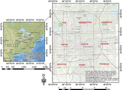
The study area, Marion County, Indiana, is located in the Midwest USA (Figure 2). It is the county seat of Indianapolis, the capital and largest city in the State of Indiana. Marion County is part of the Indianapolis–Carmel–Anderson metropolitan statistical area. It covers both the urban and suburban areas of the city of Indianapolis. The county is located on a flat plain, which makes it possible for the city to expand in all directions.

Figure 2. The location of the study area, Marion County, Indiana, USA, and the nine townships in Marion County.

3.2. Dataset

3.2.1. Data for linear spectral mixture analysis

Landsat 8 images that overpass path 21 row 32 on 1 May and 18 June 2013 were used for applying linear spectral mixture analysis (LSMA) and producing images of the percentage of vegetation in each pixel. The percentage of impervious surfaces is from National Land Cover Database (NLCD) 2011. Local climate information was acquired from Indiana State Climate office (iClimate.org). USGS provides LEDAPS-processed surface reflectance for Landsat 8 scenes acquired from 11 April 2013. Therefore, the atmospheric correction was processed by USGS.

3.2.2. Data for downscaling TIR images

GOES-13 bands 4 and 6 images, one for each hour, from 20 June to 30 June 2013, were downloaded from the National Oceanic and Atmospheric Administration (NOAA) comprehensive large array-data stewardship system (http://www.nsof.class.noaa.gov/saa/products/search?datatype_family=GVAR_IMG). There are two locations for GOES satellites: East and West (http://www.nsof.class.noaa.gov/release/data_available/goes/index.htm). Our study area was covered by the GOES satellites at the East location. During 2013, GOES13-Imager was the one covering the East half of the earth. Therefore, GOES13-Imager was chosen in this study. MODIS daily LST images from September to November, 2013, were downloaded from Earth Explorer (http://earthexplorer.usgs.gov/). The auxiliary data for downscaling GOES to MODIS resolution included vegetation indices, albedo, emissivity, elevation, and percent of imperviousness. Vegetation includes MODIS NDVI and enhanced vegetation index (EVI) data products, albedo in visible, near-infrared (NIR), and short-wave bands and emissivity in MODIS bands 31 and 32 were selected as auxiliary data. In addition, the Shuttle Radar Topography Mission (SRTM) digital elevation data were used to represent the terrain effects. The percentage of imperviousness data in 2011 was downloaded from the NLCD and was resampled to a 1-km resolution. The auxiliary data for downscaling MODIS to Landsat resolution were the same, except that coarser resolution data were resampled into 30-m resolution, and NDVI and fractional vegetation cover was derived from Landsat images.

3.2.3. Data for soil moisture estimation

The downscaled LST and fractional vegetation cover were used in soil moisture estimation. Soil type data for Marion County were acquired from Indianapolis Mapping and Geographic Infrastructure System (IMAGIS). Air temperatures were requested from weather stations on Indiana State Climate office (iClimate.org). Vegetation indices and fractional vegetation cover were calculated from Landsat 8 images.

3.2.4. Data for displacement height and roughness length estimation

For buildings, digital elevation model (DEM), digital surface model (DSM), building footprint, and land use types in Marion County at parcel level in 2010 were requested from IMAGIS. It was reclassified for the purpose of validating and comparing the estimated roughness length and displacement height with existing literatures. In addition, 2010 TIGER Census Block shapefiles have been downloaded from Census.gov.

3.2.5. Data for ET estimation

Hourly solar radiation data were acquired from the National Solar Radiation Database (http://rredc.nrel.gov/solar/old_data/nsrdb/). Daily solar radiation was configured by averaging hourly data. Hourly wind speed, atmospheric temperature, air pressure, and relative humidity were acquired from the Indiana State Climate office (iClimate.org). The data were collected in the International Airport of Indianapolis. Percent of Imperviousness was downloaded from NLCD 2011. Fractional vegetation cover data configured by LSMA in previous sections. LSTs were downscaled from GOES to MODIS resolution and from MODIS to Landsat resolution. DEM and DSM were used to produce roughness length for both momentum and heat and displacement height.

3.3. Methodology

The following figure shows the work flow of the methodology section (Figure 3). First, the LST data were downscaled to produce 1-km resolution hourly LST, and 30-m resolution daily LST. Second, the LSMA was applied, and the land surface was depicted by three major components: vegetation, soil, and impervious surfaces. In each pixel, the combination of land surfaces was described by percentages of the three components. Third, the volumetric soil moisture was calculated by temperature vegetation index (TVX) method. Fourth, the energy balance model was formed, and the ET was calculated. Fifth, urban morphology, such as the frontal area of buildings and trees that face the wind direction, was calculated, and the roughness length for momentum and heat transport was estimated and embedded into the energy balance model. Lastly, a sensitive analysis and field work validation were conducted.

Figure 3. The flowchart of general methodology.

3.3.1. LST computation

LST was computed by Split Window (SW) algorithm for GOES images, because it has two thermal bands located in the atmospheric window between 10 and 12 μm. The SW algorithms and the coefficients were adopted from Jiménez-Muñoz and Sobrino (2008) for GOES. The equation of the algorithm can be written as

(1)

where and are the at-sensor brightness temperature at the SW bands and in kelvins, is the mean emissivity , is the emissivity difference , is the total atmospheric water vapor content in , and are the SW coefficients determined from simulated data.

3.3.2. LST downscaling

The downscaling method follows Zakšek and Oštir (2012). First, principal component analysis (PCA) was applied on auxiliary data in 1-km spatial resolution; second, the highest ranked principal components were upscaled to 4 km; third, regressions between GOES LST and selected components were formed; lastly, the LSTs in 1-km spatial resolution were be estimated. For the hourly estimation, the LSTs are downscaled from 4-km GOES resolution to 1-km MODIS resolution; for daily estimation, the LSTs are downscaled from 960-m MODIS resolution to 240 m, and then from 240 to 30 m Landsat resolution.

Data were divided into two categories: temperature and auxiliary data. The GOES-13 Imager possesses five spectral bands, one visible band at 0.54–0.71 µm, and four infrared bands at 3.73–4.08, 5.90–7.28, 10.19–11.18, and 13.01–13.71 µm, respectively. The data were downloaded from the NOAA comprehensive large array-data stewardship system (http://www.nsof.class.noaa.gov/saa/products/search?datatype_family=GVAR_IMG). The NOAA Weather and Climate Toolkit was used to export the AREA files to tiff format. AREA files are count data with calibration coefficients. The toolkit uses the calibration information contained in the calibration block of the AREA file and converts the raw counts (10 bit precision) to brightness temperatures for the IR channels. Then, GOES LSTs were retrieved using the SW algorithm and coefficients from Jiménez-Muñoz and Sobrino (2008).

Since LST is strongly influenced by parameters as solar irradiation, albedo, topography, thermal inertia, and vegetation cover (Weng, Lu, and Schubring 2004), auxiliary data were obtained for downscaling. The auxiliary data related to vegetation included MODIS NDVI and EVI data products. Albedo in visible, NIR, and shortwave bands and emissivity in MODIS bands 31 and 32 were also selected. In addition, the SRTM digital elevation data were used in the downscaling. The percentage of imperviousness data in 2011 was downloaded from NLCD and was resampled to 1-km resolution.

3.3.3. VIS model

LSMA was applied to derive fractional vegetation cover. The fractional vegetation cover was calculated according to scaled NDVI, because the data used in this study span from summer to winter, the vegetation cover changed and it will be hard to keep the accuracy by selecting end members manually at the vertices of PCA bands scatter plots. The equation of calculating fractional vegetation cover can be written as

(2)

where is the minimum value of NDVI and is the maximum value of NDVI.

The percentage of impervious surface was based on the NLCD2011 Percent of Imperviousness. We assume that each pixel consists of vegetation, impervious surface, and soil. Therefore, besides the percentage of vegetation and impervious surfaces, the rest of the land in each pixel was assumed to be soil.

3.3.4. Soil moisture estimation

Soil moisture was retrieved based on surface energy balance modeling (Jiang and Islam 2001; Rahimzadeh-Bajgiran et al. 2013). First, the extension of the Priestley–Taylor parameter (Jiang and Islam 2001) was estimated in the TVX space; second, based on the results, the evaporative fraction was calculated; finally, the volumetric soil moisture was computed based on its relationship with the evaporative fraction (Rahimzadeh-Bajgiran et al. 2013).

The detailed description of the TVX space can be found in Carlson and Arthur (2000). In this case, φ is the extension of the Priestley–Taylor parameter α. can be written as

(3)

where is the maximum scaled LST, is the minimum. is the maximum value, and is the minimum. and are the LST and values of pixel i. LST was transformed to scaled LST before the TVX space was formed. The equation for transforming LST to scaled LST was written as

(4)

Then, the evaporative fraction can be estimated by the following equation:

(5)

where is the extension of the Priestley–Taylor parameter α and is air temperature control parameter (Jiang and Islam 2001). In this study, the maximum value of (under the wet surface condition) was assumed to be 1.26 and the minimum was 0 (under the dry surface condition). was estimated using a linear function with air temperature (Wang, Li, and Cribb 2006).

The method to calculate soil moisture from evaporation fraction was adapted from Lee and Pielke (1992):

(6)

where θ is volumetric soil moisture, EF is evaporative fraction, and is volumetric soil moisture at field capacity. Silt loam and clay loam were commonly found in our study area (Sturm and Gilbert 1978). Based on the soil–water characteristics of different soil types in Lee and Pielke (1992), was assumed to be 0.3.

3.3.5. Estimating displacement height and roughness length using DEM and DSM

The method of estimating displacement height and roughness length was adopted from Burian et al. (2002, 2003a, 2003b), and the estimation is based on height, frontal area, and building plan area fraction. DSM and DEM derived from airborne Terrestrial Light Detection and Ranging (LiDAR) data were used to estimate the building heights. The average height of DSM and DEM within each building polygon was extracted, and the difference between the two is building height. Since the LiDAR was collected in 2009, and the building polygon data were updated in 2013, not all building polygons had corresponding buildings when LiDAR was taken. Therefore, only buildings greater than 3 m were selected in the following analysis. We used 3 m as the criterion, because, in this area, most commercial properties have flat roofs, they are 12 ft per floor; and most residential properties have slanted roofs, and they are 10 ft per floor and 10 ft for the roof. Therefore, the buildings should be greater than 3 m.

The building plan area fraction is calculated as the building plan area divided by the total plan area. The frontal area is the total area of buildings projected into the plane normal to the approaching wind direction. The frontal area index can be calculated by the frontal area divided by total plan area. Although the average wind direction in Indianapolis is SW, the majority of streets are in North–South or East–West direction, and the wind at this height follows the direction of streets. Building frontal area facing north was used in the following calculation.

The Macdonald method (Macdonald, Griffiths, and Hall 1998) was chosen because it was modified from the one representing rounded obstacles to more rectangular and greater building plan area. Therefore, it is good to represent buildings.

(7)

(8)

where is the height of the building, α is an empirical coefficient, (=1.2) is a drag coefficient, k is von Karman’s constant, and β is a correction factor for the drag coefficient. According to the sensitivity analysis in Macdonald, Griffiths, and Hall (1998), the value for α and β is 4.43 and 1.0, respectively. is the building plan area fraction, and is the building frontal area index.

Considering the seasonal change of tree morphology, the tree morphological data that estimated from terrestrial LiDAR was from September 2013 which covered Warren Township, Indianapolis. The displacement height and roughness length were calculated using tree height and tree frontal area based on the Raupach (1994). The details of Raupach method can also be found in Grimmond and Oke (1999) and Burian, Han, and Brown (2003a). The Raupach (1994) method can be written per the following equations:

(9)

(10)

(11)

where is the roughness sublayer influence function, U is the large-scale wind speed, and is the friction velocity. and are drag coefficients for the substrate surface at height in the absence of roughness elements and of an isolated roughness element mounted on the surface, respectively. is a free parameter. is the building plan area fraction, is the building frontal area index. According to Raupach (1994), , , , , and . Raupach (1994) method was chosen because it was originally designed to calculate displacement height and roughness length as functions of canopy height and area index for vegetation. The displacement height and roughness length were added to the layers of building morphological data and used in the surface moisture model.

3.3.6. The land surface moisture model

The method of estimating LE followed Weng et al. (2013) and Kato and Yamaguchi (2007). Net radiation was calculated according to shortwave radiation, broadband albedo, surface emissivity, atmospheric emissivity, air temperature from weather stations, and surface temperature from downscaling. The equation is as follows:

(12)

where is the net radiation, is the Stefan–Boltzmann constant , is atmospheric emissivity, is broadband albedo, is shortwave radiation, is surface broadband emissivity, is atmospheric temperature, and is surface temperature.

Atmospheric emissivity was calculated as

(13)

where is the atmospheric water vapor pressure. Broadband albedo was calculated according to Liang (2000), and broadband emissivity was calculated according to Ogawa et al. (2003).

Ground heat flux was calculated based on net radiation and a coefficient that describes the influence of surface cover material, seasonality, and diurnal change. The land cover was classified into water, bare soils, grass, forest, urban, and agriculture, and values vary among different land cover types. The equation is as follows:

(14)

In this original model, the values were adopted from Table 2 in Weng et al. (2013), because the study area was the same. The values can be found in Table 3.

Table 3. Values according to LULC types for ground heat flux.

LULC types
Water	0.35
Bare soils	0.30
Grass	0.30
Forest	0.15
Urban	0.40
Agriculture	0.30

Sensible heat flux was calculated as

(15)

where is the air density in kg/m³, is the specific heat of air at constant pression in J/(kg K), is the surface temperature for non-vegetated areas and is the surface temperature for vegetated areas, and is the air temperature. is the aerodynamic resistance in s/m. The aerodynamic resistance was calculated by displacement height and roughness lengths for momentum and heat transport. was calculated as

(16)

where is the displacement height. and are the roughness lengths for momentum and heat transport. In the original model, the parameters describing the roughness condition of land surface, namely , , and , were fixed according to the LULC types that were estimated in existing literature. Although each land cover type may yield similar morphological parameters, each city has its own unique morphological characteristics, which relate to history, culture, tradition, planning, and topography; it varies over regions, countries, and continents as well. Contexts that impact the urban setting include hydraulic factors, transportation hubs, trade centers, defensive sites, and religious factors. Therefore, in this study, these parameters were estimated using DEM and DSM data (Burian, Han, and Brown 2003a). According to Weng et al. (2013), and are the heights at which the wind speed and atmospheric temperature are measured. and are 10 and 2 m, respectively. and are stability correction functions for momentum and heat, and k is von Karman’s constant, which equals 0.4. This equation may be simplified by removing and (Weng, Fu., and Gao 2014).

Latent flux (LE), also known as ET, will also be calculated for vegetated and non-vegetated areas separately. The total LE was described by the following equation:

(17)

where and are used to differentiate the vegetated and non-vegetated areas. In this article, 0.5 was used as the threshold. The , LE from non-vegetated areas, was estimated by subtracting G and from on non-vegetated surfaces. It can be expressed by

(18)

The , LE over vegetated areas, was estimated by the following equation:

(19)

where is the Priestley–Taylor parameter, which equals 1.26, γ is psychrometric constant, is the slope of saturation vapor pressure–temperature curve. is the fraction of the leaf area index that is green, and it equals unity when it is not available. If is negative, it was set to zero, was recomputed as the residual of Equation (18).

When the LE is greater than zero, the LE estimates at the sensor overpass time were converted to daily daytime ET, assuring a self-preservation of the evaporative fraction during daytime hours: (Cammalleri et al. 2014). A correction multiplicative coefficient of 1.1 for was introduced for a 10% systematic underestimation of daytime average from values estimated around midday (Cammalleri et al. 2014).

4. Results

4.1. Percentage of soil, vegetation, and impervious surface in each pixel

In this study, we considered the pixels with 90% or more of certain land cover type (vegetation, soil, or impervious surfaces) as pure pixels. On 6 September, 94,533 out of 1158,956 pixels were pure vegetation, 9 pixels were pure soil. On 8 October, 27,072 pixels were pure vegetation, and 449 pixels were pure soil. On 9 November, 2384 pixels were pure vegetation, and 312 pixels were pure soil. According to NLCD2011, there were 43,673 pure impervious surfaces pixels. The spatial distribution of the three land cover types on three satellite over-pass days is showed in Figure 4.

Figure 4. Fractions of vegetation, soil, and impervious surfaces in each pixel and the distribution of pure pixels. The fractions of vegetation and soil were from Landsat 8 acquired on DOY 249 (6 September), 281 (8 October), and 313 (9 November), 2013, and the fraction of impervious surface was from NLCD2011 data. The spatial resolution is 30 m.

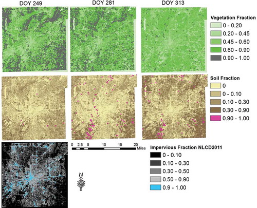
In this study, the pixels with 90% or above of certain land cover are considered to be pure pixels, and the ET was compared between the three categories of pure pixels, namely vegetation, soil, and impervious surfaces. The contrastive colors in Figure 3 were to show the locations of the pure pixels. In September, the DOY249 image shows large amount of pure vegetation pixels (in gray) in the forest areas along the Eagle Creek Reservoir and Geist Reservoir, the low-density residential areas in the north side of Indianapolis, and the agricultural fields in the South of Indianapolis. In October, the pure vegetation pixels decreased dramatically in agricultural fields; in November, the limited pure vegetation pixels scattered in the DOY313 image. On the contrary, in September, the pure soil pixels (in pink) were very limited, but in October and November, the pure soil pixels increased along White River, and the pixels with higher percentage of soil further increased in agricultural and forest areas. In blue shows the distribution of pure impervious surfaces in NLCD 2011 image; the pure impervious surfaces pixels were located along major roads and interstate highway, as well as Central Business District (CBD), shopping mall, and big infrastructures.

4.2. Displacement height and roughness length from buildings

Compared to the empirical values displacement height and roughness length that estimated according to land use and land cover types, the estimates from DEM and DSM represented a more realistic scenario (Figure 5). It did not assign the large portion of built-up areas with the same value but captured higher variation between blocks in the land use and land cover type. The highest displacement height values were found in the CBD, followed by commercial areas and high density residential. The highest roughness length values were found in the coal-mining site near the power plant, followed by CBD and high density residential areas. The displacement height and roughness length of trees were estimated in Warren Township. We did not show figure separately here, because the roughness values from trees are significantly smaller than buildings, which is due to the transparency of trees.

Figure 5. Displacement height (a) and roughness length (b) in meters from buildings.

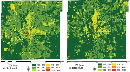
In Kato and Yamaguchi (2007) and Weng et al. (2013), empirical values of surface roughness were used to estimate heat fluxes such as net radiation, ground heat flux, sensible heat flux, and latent heat flux. Since the study area of Weng et al. (2013) was also Indianapolis, Indiana, the airborne LiDAR-derived surface roughness and the empirical values were compared. Weng et al. (2013) categorized the land cover into six types: water, bare soil, grass, forest, urban, and agriculture. The displacement height value was based on Kustas et al. (2003). The area categorized as urban were given the uniformed value 1.95, and the area categorized as agriculture and grass were given the value 0.1. The uniformed displacement height or roughness length values were not as accurate. Although the average displacement height value of urban area is close to 1.95 m, the highest point yielded 46.47 m, which is 2383% different from the average value. According to the DEM and DSM from LiDAR data, the downtown core areas would yield much higher displacement height, industrial sites and residential area have different morphological characteristics, and even residential areas can be further categorized based on its density. Not to mention the dramatic variations between commercial and transportation areas. Therefore, using coarse land cover classification and assigning empirical values may lead to inaccurate estimation in surface fluxes estimation.

Finer classifications would be more accurate. For example, Kato and Yamaguchi (2007) classified land cover in to 15 types. They were able to differentiate tall trees and low trees, dense grass and sparse grass, flat pavement and road, and high-rise and low-rise. However, in each category, the assigned value was an average for the whole category, not the actual measure. This matters because for the same land cover classes, the parameters may vary in different locations and for different purpose. For example, industrial areas in urban areas and suburb areas may show different morphological characteristics, and car manufacturing and electronic industry may also show big difference. Therefore, using LiDAR-derived DEM and DSM to model the surface roughness is more accurate than using empirical values based on LULC types, and it will improve the accuracy of surface fluxes and moisture estimation as well.

4.3. Hourly soil moisture and ET estimated from downscaled GOES LST

The hourly estimates of soil moisture and ET are not the average of each hour, but the instantaneous value of the downscaled LST. The hourly soil moisture was estimated from the downscaled GOES LST from 4 to 1 km from 20 to 30 June 2013. Since in urban areas it is hard to find pure soil pixels at the size of 1 km × 1 km, a pixel with 85% or higher percentage of soil was considered pure soil pixels. The hourly soil moisture in the study area fluctuated between 15% and 20% and do not show an obvious correspondence with the precipitation (Figure 6(a)). Although there is more than 2-cm precipitation on 23 June and less than 0.5-cm precipitation, on 25 June, 26 June, 29 June, and 20 June, the soil moisture did not show dramatic changes immediately before and after precipitation. About 24 h later, it showed slight increases of peak values. This indicates the water retention capacity of soil: it absorbs and transports extra water right after the precipitation. The previous study on soil moisture by Rahimzadeh-Bajgiran et al. (2013) showed that the soil moisture in the Canadian Prairies in parts of Saskatchewan and Alberta was 12–22%, and the study on soil moisture in Indianapolis, Indiana by Jiang, Fu, and Weng (2015), showed that the soil moisture in this area was 16–20% in 2001 and 2006. Therefore, the range of soil moisture is reasonable in this study. Although field-measured soil moisture data are needed to further validate the results, the estimation of soil moisture using thermal infrared remote sensing and downscaling technique is useful to monitor the changes of soil moisture in urban areas with heterogeneous land cover types.

Figure 6. Hourly soil moisture (a) and hourly LE from soil, vegetation, and impervious surfaces (b) from 20 June to 30 June 2013.

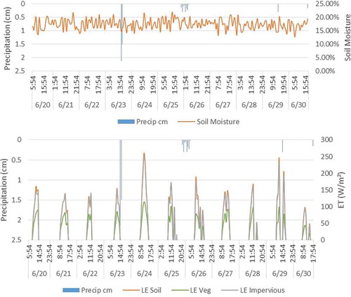
The evaporation and transpiration from vegetation, soil, and impervious surfaces shows different patterns before and after precipitation (Figure 6(b)). The pattern of ET from soil and impervious surfaces was similar, with slightly higher ET from soil surfaces. It was expected that impervious surfaces could show different patterns than soil surfaces. However, due to the frequent precipitation in June, 2013, the ET over impervious surfaces stayed high. According to the Indiana State Climate Office (iclimate.org), the recent precipitations before 20 June were on a 9-h rainfall on 16 June, followed by another precipitation on 17 June. In between the precipitations, the ET from the soil and impervious surfaces were between 150 and 200 W/m². After the precipitation on 23rd June, the LE of the soil and impervious surfaces increased dramatically and reached 250 W/m². Another reason for the similar pattern of ET on soil and impervious surfaces is that this estimation was based on LST downscaled from 4 to 1 km, it is hard to guarantee that pure soil or impervious surfaces was found in a 1-km² area, given the heterogeneity of urban land covers. Compared to soil and impervious surfaces, ET from vegetation surfaces was more stable and did not change much before or after precipitation. The peak value during the day was 50–100 W/m².

4.4. Daily soil moisture and ET estimated from downscaled MODIS LST

The daily soil moisture and ET were estimated in the fall and winter season from September to November, 2013. They are not daily average, but the instantaneous estimates at the MODIS passing time. Compared to hourly soil moisture, daily soil moisture shows more variations to precipitation and temperature (Figure 7(a)). The general trend of soil moisture decreased slightly from September to November, although there is more precipitation in the winter months. This trend is more obvious in October to November. Soil moisture also showed the corresponding changes before and after precipitation. For example, after the precipitation before DOY 265, there was a clear increase followed by a drop of soil moisture between DOY 265 and 270. During the precipitations between DOY 270 and 280, the soil moisture increased slowly. After the 2-cm precipitation on DOY 305, the soil moisture increased again.

Figure 7. Daily soil moisture (a) and daily ET over vegetation, soil, and impervious surfaces (b) from September to November in 2013.

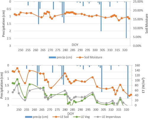
Similar to the soil moisture, the ET estimates from three land cover surfaces showed a decreasing trend from September to November (Figure 7(b)). This is due to the decrease of solar irradiation, air temperature, and LST. Similar to the hourly ET estimation in summer 2013, soil surfaces yielded the highest ET in September to November as well. ET from vegetation showed a similar pattern as soil surfaces, although the amount is much smaller. Impervious surfaces show different responses to precipitation. For example, during the precipitation between DOY 260 and 265, the ET from impervious surfaces shows a more rapid increase than vegetation and soil surfaces. However, after DOY 280, a decrease of ET was shown on three land cover types. This decrease is because in the months of September to November, precipitation becomes a less important factor to impact ET, and the temperature due to seasonal change becomes more influential.

The spatial distribution of ET from DOY 281 to 318 with a roughly 5-day interval was shown at 30-m resolution in Figure 8(a). The highest ET was usually found in bodies of water, agriculture fields in the southern part of the county, and forests. On DOY 281, 291, 298, and 307, the central urban area yielded high ET, because these days were shortly after the precipitation.

Figure 8. Spatial distribution of ET: (a) for the whole study area from DOY 281 to 318, 2013; (b) comparison between the central urban area and the city’s average.

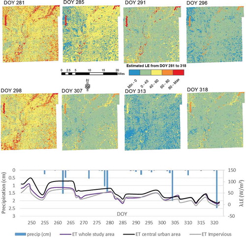
In the whole study area, the displacement height and roughness length were derived only from buildings; the surface roughness from soil and vegetation was not considered in the moisture estimation. Therefore, to investigate the impact of surface roughness on surface moisture, we chose a central urban area that yielded the highest displacement height: the area with displacement height greater than 10 m was selected. The result was compared with the average ET in the whole study area in Figure 8(b). The results show that the ET from central urban area was higher than that from the whole study area from September to November. It may be because the relatively higher temperature from anthropogenic heat in the offices and commercial buildings in the central urban area accelerate the evaporation. The difference was found greater in September and smaller in November. It is because the temperature is lower in November, and the ET in both central urban area and the surrounding area becomes slower compared to September. From DOY 305 to 320, the ET was almost the same. The trend and the response to precipitation were similar.

ET that estimated with building morphological data was compared with ET with combined building and tree morphological data in Warren Township. The result showed that tree morphological data affected little of the ET estimates from soil and impervious surfaces. The sample area, along the Lick Creek in Warren County, Indianapolis, has relatively big trees; however, due to the transparency of trees, they do not have a big impact on aerodynamic resistance compared to buildings.

5. Discussion

The major contribution of this study is to use the morphological data that derived from Terrestrial LiDAR in a two source energy balance (TSEB) model, and the results were compared with the morphological data that estimated from empirical values. The morphological data are important for urban surface moisture estimation because roughness length and displacement height impact wind direction and wind speed, and consequently surface moisture (Jiang et al. 2016). The limitation of the research and the future directions are discussed below.

In this research, displacement height, roughness length for momentum, and roughness length for heat were calculated from DEM and DSM. Among the three parameters, roughness length for heat was calculated based on its relationship with average building heights (Sugawara and Narita 2009). To keep the procedure simple and to consider the large influence from anthropogenic heat (Sugawara and Narita 2009), we did not consider the diurnal variation of in this study. Therefore, more study is needed to consider anthropogenic heat in estimation, as well as in LE estimation.

The method of estimating ET is applicable when the air temperature is higher than 0°C. In the estimation of atmospheric emissivity, the division of atmospheric water vapor pressure and air temperature must be greater than 0 to have a fractional power. Also, water does not evaporate under 0°C, and stomata of vegetation remain closed and stop transpiration at low temperatures. Therefore, in this study, the days with a negative air temperature, which only occurred in November, were eliminated from the surface moisture estimation.

Lacking field data for validation, the estimation of the soil moisture and ET were compared with previous studies from Rahimzadeh-Bajgiran et al. (2013) and Weng et al. (2013), respectively. According to Weng et al. (2013), the average ET on 3 October 2000 was 101 W/m² with a standard deviation of 66 W/m² in Indianapolis, Indiana in the fall season. The highest ET was from water bodies with an average of less than 300 W/m², followed by bare soil with an average of 200 W/m², vegetated area yielded 150 W/m², and the lowest ET is from urban land which contributed less than 100 W/m². In the summer season, the average of ET on 16 June 2001 was 195 W/m², with a standard deviation of 94 W/m². The ET was higher than 300 W/m² from bare soil, between 200 and 300 W/m² from vegetation and between 100 and 200 W/m² from urban land. In the current study, in October, the average ET from soil was 100.15 W/m² with a standard deviation of 14.35 W/m². The average ET from vegetation was 23.85 W/m² with a standard deviation of 15.53 W/m². The average ET from impervious surfaces was 35.32 W/m², with a standard deviation of 12.41 W/m². The average ET from vegetation is lower, because it is a monthly average instead of a value from a single day at the beginning of October in Weng et al. (2013). The impervious surfaces yielded higher ET because the images were acquired in a rainy period, and one of the purposes of the study was to investigate the behavior of impervious surfaces on evaporation after precipitation. In the summer season, the LE results estimated from calculated roughness length and displacement height values were compared with the ET results that estimated with empirical values of roughness length and displacement height over soil, impervious surfaces, and central urban areas. Vegetation surfaces were not included in the comparison because the ET for vegetation was generated according to net flux and ground flux without considering the surface roughness (Equation 12). The results showed that the ET estimations are almost the same from the two approaches, especially for soil and impervious surfaces. The R² was close to 1 and the RMSEs were 0.18 and 0.14 W/m² for soil and impervious surfaces, respectively. Slight larger differences were found in central urban areas with the surface roughness contributed by tall buildings, and the RMSE was 0.64 W/m². This result showed that the calculated surface roughness values did not produce ET results that deviate from the estimation from empirical values.

6. Conclusions

This study used hourly LST downscaled from GOES to MODIS resolution and daily LST downscaled from MODIS to Landsat resolution to estimate the soil moisture and ET in urban areas. In particular, this study used calculated surface roughness values from DEM and DSM in TSEB model. The results of this study showed the fluctuating, yet stable, hourly soil moisture ranged from 15% to 20% before and after precipitation in summer time; the increase of daily soil moisture toward precipitation and decreasing trend due to seasonal temperature changed from fall to winter. Also, soil, vegetation, and impervious surface in urban areas yielded different patterns in response to precipitation, which indicated the contribution of impervious surface to evaporation in urban areas. Moreover, in the central urban area, where the surface roughness is mainly contributed by high-rise, the evaporation and transpiration is higher than the average of the whole city. However, by adding the roughness parameters from trees, the surface moisture did not yield a significant difference, even in the residential area where there are lots of trees. This study showed that the downscaled LST is capable of capturing the ET over heterogeneous urban surfaces, and the combination of downscaled LST, surface roughness values from DEM and DSM, and TSEB model is a valid approach to the study on ET in urban areas.

Disclosure statement

No potential conflict of interest was reported by the authors.

References

- Agam, N., W. P. Kustas, M. C. Anderson, F. Li, and C. M. U. Neale. 2007. “A Vegetation Index Based Technique for Spatial Sharpening of Thermal Imagery.” Remote Sensing of Environment 107: 545–558. doi:10.1016/j.rse.2006.10.006.
- Bartens, J., S. D. Day, J. R. Harris, T. M. Wynn, and J. E. Dove. 2009. “Transpiration and Root Development of Urban Trees in Structural Soil Stormwater Reservoirs.” Environmental Management 44: 646–657. doi:10.1007/s00267-009-9366-9.
- Boegh, E., H. Soegaard, N. Hanan, P. Kabat, and L. Lesch. 1999. “A Remote Sensing Study of the NDVI–Ts Relationship and the Transpiration from Sparse Vegetation in the Sahel Based on High-Resolution Satellite Data.” Remote Sensing of Environment 69: 224–240. doi:10.1016/S0034-4257(99)00025-5.
- Burian, S. J., M. J. Brown, and S. P. Linger. 2002. Morphological Analyses Using 3D Building Databases. Los Angeles, CA: Los Alamos National Laboratory.
- Burian, S. J., W. S. Han, and M. J. Brown. 2003a. Morphological Analyses Using 3D Building Databases. Houston, TX: Los Alamos National Laboratory.
- Burian, S. J., W. S. Han, and M. J. Brown. 2003b. Morphological Analyses Using 3D Building Databases. Oklahoma City, OK: Los Alamos National Laboratory.
- Cammalleri, C., M. C. Anderson, F. Gao, C. R. Hain, and W. P. Kustas. 2014. “Mapping Daily Evapotranspiration at Field Scales over Rainfed and Irrigated Agricultural Areas Using Remote Sensing Data Fusion.” Agricultural and Forest Meteorology 186: 1–11. doi:10.1016/j.agrformet.2013.11.001.
- Carlson, T. N., and S. T. Arthur. 2000. “The Impact of Land Use — Land Cover Changes Due to Urbanization on Surface Microclimate and Hydrology: A Satellite Perspective.” Global and Planetary Change 25: 49–65. doi:10.1016/S0921-8181(00)00021-7.
- Christensen, L., C. L. Tague, and J. S. Baron. 2008. “Spatial Patterns of Simulated Transpiration Response to Climate Variability in a Snow Dominated Mountain Ecosystem.” Hydrological Processes 22: 3576–3588. doi:10.1002/hyp.v22:18.
- Fleetwood, Å., and I. Larsson. 1968. “Precipitation, Soil Moisture Content and Ground Water Storage in a Sandy Soil in Southern Sweden.” Oikos 19: 234–241. doi:10.2307/3565010.
- Grimmond, C. S. B., and T. R. Oke. 1999. “Aerodynamic Properties of Urban Areas Derived from Analysis of Surface Form.” Journal of Applied Meteorology 38: 1262–1292. doi:10.1175/1520-0450(1999)038<1262:APOUAD>2.0.CO;2.
- Hagishima, A., K.-I. Narita, and J. Tanimoto. 2007. “Field Experiment on Transpiration from Isolated Urban Plants.” Hydrological Processes 21: 1217–1222. doi:10.1002/(ISSN)1099-1085.
- Hilker, T., F. G. Hall, N. C. Coops, J. G. Collatz, T. Andrew Black, C. J. Tucker, P. J. Sellers, and N. Grant. 2013. “Remote Sensing of Transpiration and Heat Fluxes Using Multi-Angle Observations.” Remote Sensing of Environment 137: 31–42. doi:10.1016/j.rse.2013.05.023.
- Husain, S. Z., S. Bélair, and S. Leroyer. 2014. “Influence of Soil Moisture on Urban Microclimate and Surface-Layer Meteorology in Oklahoma City.” Journal of Applied Meteorology and Climatology 53: 83–98. doi:10.1175/JAMC-D-13-0156.1.
- Inamdar, A., and A. French. 2009. “Disaggregation of GOES Land Surface Temperatures Using Surface Emissivity.” Geophysical Research Letters 36: L02408. doi:10.1029/2008GL036544.
- Jiang, L., and S. Islam. 2001. “Estimation of Surface Evaporation Map over Southern Great Plains Using Remote Sensing Data.” Water Resources Research 37: 329–340. doi:10.1029/2000WR900255.
- Jiang, Y., P. Fu, and Q. Weng. 2015. “Assessing the Impacts of Urbanization Associated Land Use/Cover Change on Land Surface Temperature and Surface Moisture: A Case Study in the Midwestern United States.” Remote Sensing 7: 4880–4898. doi:10.3390/rs70404880.
- Jiang, Y., Q. Weng, J. H. Speer, and S. Baker. 2016. “Estimating Tree Frontal Area in Urban Areas Using Terrestrial LiDAR Data.” Remote Sensing 8 (5): 401. doi:10.3390/rs8050401.
- Jiménez-Muñoz, J., and J. A. Sobrino. 2008. “Split-Window Coefficients for Land Surface Temperature Retrieval from Low-Resolution Thermal Infrared Sensors.” IEEE Geoscience and Remote Sensing Letters5: 806–809. doi:10.1109/LGRS.2008.2001636.
- Kato, S., and Y. Yamaguchi. 2007. “Estimation of Storage Heat Flux in an Urban Area Using ASTER Data.” Remote Sensing of Environment 110: 1–17. doi:10.1016/j.rse.2007.02.011.
- Kjelgren, R., and T. Montague. 1998. “Urban Tree Transpiration over Turf and Asphalt Surfaces.” Atmospheric Environment 32: 35–41. doi:10.1016/S1352-2310(97)00177-5.
- Kustas, W. P., A. N. French, J. L. Hatfield, T. J. Jackson, M. S. Moran, A. Rango, J. C. Ritchie, and T. J. Schmugge. 2003. “Remote Sensing Research in Hydrometeorology.” Photogrammetric Engineering & Remote Sensing 69: 631–646. doi:10.14358/PERS.69.6.631.
- Lee, T. J., and R. A. Pielke. 1992. “Estimating the Soil Surface Specific-Humidity.” Journal of Applied Meteorology 31: 480–484. doi:10.1175/1520-0450(1992)031<0480:ETSSSH>2.0.CO;2.
- Liang, S. 2000. “Narrowband to Broadband Conversions of Land Surface Albedo I: Algorithms.” Remote Sensing of Environment 76: 213–238.
- Macdonald, R. W., R. F. Griffiths, and D. J. Hall. 1998. “An Improved Method for the Estimation of Surface Roughness of Obstacle Arrays.” Atmospheric Environment 32: 1857–1864. doi:10.1016/S1352-2310(97)00403-2.
- Monteith, J. L. 1965. “Evaporation and Environment.” Symposia of the Society for Experimental Biology 19: 205–224.
- Ogawa, K., T. Schmugge, F. Jacob, and A. French. 2003. “Estimation of Land Surface Window (8–12 Μm) Emissivity from Multispectral Thermal Infrared Remote Sensing- A Case Study in A Part of Sahara Desert.” Geophysical Research Letters 302: 1067. doi:10.1029/2002GL016354.
- Pataki, D. E., H. R. McCarthy, E. Litvak, and S. Pincetl. 2011. “Transpiration of Urban Forests in the Los Angeles Metropolitan Area.” Ecological Applications 21: 661–677. doi:10.1890/09-1717.1.
- Penman, H. L., and I. F. Long. 1960. “Weather in Wheat: An Essay in Micro-Meteorology.” Quarterly Journal of the Royal Meteorological Society 86: 16–50. doi:10.1002/(ISSN)1477-870X.
- Rahimzadeh-Bajgiran, P., A. A. Berg., C. Champagne, and K. Omasa. 2013. “Estimation of Soil Moisture Using Optical/Thermal Infrared Remote Sensing in the Canadian Prairies.” ISPRS Journal of Photogrammetry and Remote Sensing 83: 94–103. doi:10.1016/j.isprsjprs.2013.06.004.
- Ramamurthy, P., and E. Bou-Zeid. 2014. “Contribution of Impervious Surfaces to Urban Evaporation.” Water Resources Research 50: 2889–2902. doi:10.1002/2013WR013909.
- Raupach, M. R. 1994. “Simplified Expressions for Vegetation Roughness Length and Zero-Plane Displacement as Functions of Canopy Height and Area Index.” Boundary Layer Meteorology 71: 211–216. doi:10.1007/BF00709229.
- Ridd, M. K. 1995. “Exploring a V-I-S (Vegetation-Impervious Surface-Soil) Model for Urban Ecosystem Analysis through Remote Sensing: Comparative Anatomy for Cities†.” International Journal of Remote Sensing 16: 2165–2185. doi:10.1080/01431169508954549.
- Shaxson, T. F., and R. Barber. 2003. Optimizing Soil Moisture for Plant Production: The Significance of Soil Porosity. Rome: Food and Agriculture Organization of the United Nations.
- Strelcova, K., D. Kurjak, A. Lestianska, D. Kovalcikova, L. Ditmarova, J. Skvarenina, and Y. A. R. Ahmed. 2013. “Differences in Transpiration of Norway Spruce Drought Stressed Trees and Trees Well Supplied with Water.” Biologia 686: 1118–1122.
- Sturm, R. H., and R. H. Gilbert. 1978. “Soil survey of Marion County, Indiana.” http://www.nrcs.usda.gov/Internet/FSE_MANUSCRIPTS/indiana/IN097/0/marion.pdf
- Sugawara, H., and K. Narita. 2009. “Roughness Length for Heat over an Urban Canopy.” Theoretical and Applied Climatology 95: 291–299. doi:10.1007/s00704-008-0007-7.
- Voogt, J. A., and T. R. Oke. 2003. “Thermal Remote Sensing of Urban Climates.” Remote Sensing of Environment 86: 370–384. doi:10.1016/S0034-4257(03)00079-8.
- Wang, K. C., Z. Q. Li, and M. Cribb. 2006. “Estimation of Evaporative Fraction from A Combination of Day and Night Land Surface Temperatures and NDVI: A New Method to Determine the Priestley-Taylor Parameter.” Remote Sensing of Environment 102: 293–305. doi:10.1016/j.rse.2006.02.007.
- Weng, Q. 2009. “Thermal Infrared Remote Sensing for Urban Climate and Environmental Studies: Methods, Applications, and Trends.” ISPRS Journal of Photogrammetry and Remote Sensing 64: 335–344. doi:10.1016/j.isprsjprs.2009.03.007.
- Weng, Q., and P. Fu. 2014. “Modeling Diurnal Land Temperature Cycles over Los Angeles Using Downscaled GOES Imagery.” ISPRS Journal of Photogrammetry and Remote Sensing 97: 78–88. doi:10.1016/j.isprsjprs.2014.08.009.
- Weng, Q., D. Lu, and J. Schubring. 2004. “Estimation of Land Surface Temperature-vegetation Abundance Relationship for Urban Heat Island Studies.” Remote Sensing of Environment 89 (4): 467–483.
- Weng, Q., P. Fu., and F. Gao. 2014. “Generating Daily Land Surface Temperature at Landsat Resolution by Fusing Landsat and MODIS Data.” Remote Sensing of Environment 145: 55–67. doi:10.1016/j.rse.2014.02.003.
- Weng, Q., X. Hu, D. A. Quattrochi, and H. Liu. 2013. “Assessing Intra-Urban Surface Energy Fluxes Using Remotely Sensed ASTER Imagery and Routine Meteorological Data: A Case Study in Indianapolis, U.S.A.” IEEE Journal of Selected Topics in Applied Earth Observations and Remote Sensing. doi:10.1109/JSTARS.2013.2281776.
- Weng, Q., and D. Lu. 2009. “Landscape as a Continuum: An Examination of the Urban Landscape Structures and Dynamics of Indianapolis City, 1991-2000, by Using Satellite Images.” International Journal of Remote Sensing 30: 2547–2577. doi:10.1080/01431160802552777.
- Yang, G., R. Pu, C. Zhao, W. Huang, and J. Wang. 2011. “Estimation of Subpixel Land Surface Temperature Using an Endmember Index Based Technique: A Case Examination on ASTER and MODIS Temperature Products over A Heterogeneous Area.” Remote Sensing of Environment 115: 1202–1219. doi:10.1016/j.rse.2011.01.004.
- Zakšek, K., and K. Oštir. 2012. “Downscaling Land Surface Temperature for Urban Heat Island Diurnal Cycle Analysis.” Remote Sensing of Environment 117: 114–124. doi:10.1016/j.rse.2011.05.027.