Efficient paddy field mapping using Landsat-8 imagery and object-based image analysis based on advanced fractel net evolution approach

Abstract

This paper proposes an efficient paddy field mapping method using object-based image analysis and a bitemporal data set acquired by Landsat-8 Operational Land Imager. In the proposed approach, image segmentation is the first step and its quality has a serious impact on the accuracy of paddy field classification. In order to improve segmentation quality, a new segmentation algorithm based on a frequently used method, fractal net evolution approach, is developed, with improvement mainly in merging criteria. In order to automate the process of scale parameter determination, an unsupervised scale selection method is utilized to determine the optimal scale parameter for the proposed image segmentation approach. After segmentation, four types of object-based features including geometric, spectral, textural, and contextual information are extracted and input into the subsequent classification procedure. By using a random forest classifier, paddy fields and nonpaddy fields are separated. The proposed image segmentation method and the final classification result are both quantitatively evaluated. Our segmentation method outperformed two popular algorithms according to three supervised evaluation criteria. The classification result with overall accuracy of 91.00% and kappa statistic of 0.82 validated the effectiveness of the proposed framework. Further analysis on feature importance indicated that spectral features made the most contribution as compared to the other three types of object-based features.

Keywords:

• OBIA
• FNEA
• random forest
• paddy field
• Baoying xian

1. Introduction

Rice is a major food source for most people around the world (Valipour 2014; Valipour et al. 2014; Valipour 2015; Dong et al. 2016). According to the annual report of National Bureau of Statistics of China on its portal website (National Bureau of Statistics of China, 2015), in 2014 the national gross planting area of rice amounts to more than 30 million hectares, accounting for almost 1/3 of the total grain field of the country. Consequently, rice yield has a great impact on Chinese food security and agronomic development, and the process of rice growth greatly affects the regional agro-ecological environment. Paddy field monitoring by remote sensing can provide agricultural sectors with useful information on rice growth and its geographic distribution. In this kind of task, the basic step is to accurately and reliably classify paddy fields by remote sensing data (Kobayashi et al. 2001; Shen et al. 2009; Kuenzer and Knauer 2013; Nguyen-Thanh et al. 2014; Dong et al. 2016).

It has been confirmed that remote sensing can be a valuable tool for large-area crop field observation (Hadria et al. 2010; Gumma et al. 2011; Amorós-López et al. 2013). By using remotely sensed images acquired on different dates throughout a crop cycle, crop phenology can be captured, providing meaningful cues for crop type discrimination (Panigrahy and Sharma 1997; Sakamoto et al. 2010; Nguyen-Thanh et al. 2014).

Many have investigated the active microwave remote sensing techniques for paddy field mapping (Yang et al. 2008; Wang et al. 2009; Wu et al. 2011; Sonobe et al. 2014). Although this kind of data source is immune to cloud cover, synthetic aperture radar (SAR) images are naturally speckled, leading to difficulty in their operational use. In addition, although some SAR data are freely available, the coverage of those data is quite limited, thus many researchers often cannot find the free SAR data for their study area.

On the contrary, many moderate resolution multispectral satellite images are distributed with convenient accessibility, that is, Landsat, advanced very high resolution radiometer (AVHRR), and moderate-resolution imaging spectro-radiometer (MODIS), and users can acquire those data whenever and wherever they need. Since optical sensors often suffer from cloud contamination, it will be very appealing if limited number of multispectral images can be successfully applied to paddy field mapping. A novel image analysis method, called object-based image analysis (OBIA), or geographic object-based image analysis (Blaschke 2010; Blaschke et al. 2014), may help to achieve that goal because it has many advantages over the traditional pixel-based strategy. One of its important merits is that geometric, spectral, textural, and contextual information can be used simultaneously, so that paddy fields may be classified in a more accurate way.

Many efforts have been made to agricultural mapping using OBIA (Laliberte et al. 2004; Conrad et al. 2010; Peña-Barragán et al. 2011; Lyons, Phinn, and Roelfsema 2012; Vieira et al. 2012; Kim and Yeom 2014; Peña-Barragán et al. 2014; Zhong, Gong, and Biging 2014). According to the previous works, there are three key steps in OBIA: (1) object generation, (2) object-based feature extraction, and (3) classification.

The first step is usually achieved through image segmentation. As pointed out by some literature (Vieira et al. 2012; Blaschke et al. 2014), image segmentation plays an important part in OBIA because errors can be hardly avoided in classification if geo-objects of different classes are erroneously extracted as one segment in the segmentation step. By carefully studying the previous works related to image segmentation, two aspects were found to be important for performance improvement. On the one hand, fractal net evolution algorithm (FNEA) (Baatz and Schaepe 2000) embedded in a commercial software, eCognition developer (Laliberte et al. 2004; Duro, Franklin, and Dubé 2012; Vieira et al. 2012; Zhong, Gong, and Biging 2014), was frequently used for image segmentation. Although FNEA can perform well in some cases, it may produce unsatisfactory results because its merging criterion does not incorporate any information on edge and texture, which is considered to be meaningful for image interpretation. So it is necessary to optimize the merging criterion of FNEA. On the other, scale selection for image segmentation was often done through trial-and-error, which greatly hampered the automation and objectivity in OBIA-based crop monitoring. Due to many factors, that is, farmers’ habits, local terrain characteristics, agricultural management policy, and economic conditions, the sizes of croplands vary greatly in different places, which poses difficulties in scale determination. In fact, some scale selection methods have been relatively successfully developed for FNEA and they have been rarely utilized in agricultural mapping.

Despite the difficulties in image segmentation, the significance of feature selection should not be neglected. This phase was involved with choosing the most distinctive feature(s) to assist the subsequent classification. Peña-Barragán et al. (2011) explored the use of spectral data, vegetation indices (VI) and textural features to discriminate 13 crops. They concluded that VI and spectral information was the most effective for crop type identification. Other studies also focused on using spectral features for crop type classification (Laliberte et al. 2004; Conrad et al. 2010; Kim and Yeom 2014). In this study, four types of object-based features, incorporating shape, spectra, texture and context information, were defined and extracted for crop type classification.

As for the classification step, machine learning methods, that is, decision tree (DT), random forest (RF), support vector machine (SVM), have been investigated. Vieira et al. (2012) combined OBIA and DT to map sugarcane in Brazil. After FNEA, per-field features were extracted and fed to DT algorithm. Duro, Franklin, and Dubé (2012) compared three frequently used classification methods, DT, RF, and SVM, for crop mapping. Their findings suggested that when conducting object-based classification RF and SVM outperformed DT. Zhong, Gong, and Biging (2014) also chose RF for object-based agricultural mapping and listed its major advantages that (1) RF had high prediction accuracy, (2) it could process input vectors with high dimension, and (3) it was able to automatically produce the quantitative importance of each variable. Due to the perspectives mentioned above, RF was adopted in this work.

Although there have been significant contributions presented in previous studies related to OBIA, image segmentation is still a challenging issue. How to improve the quality of image segmentation is a key factor. As mentioned above, although FNEA is a frequently adopted segmentation approach in OBIA, it fails to take into account edge and texture information that is very important in image interpretation. This paper focuses on establishing an OBIA framework for rice field mapping using advanced FNEA by combining spectral, geometric, edge, and textural information in its merging criteria to enhance segmentation quality. In addition, a recently developed method for optimal scale estimation is implemented and applied to the proposed segmentation technique in order to enhance the automation of the proposed framework. It is expected that the accuracy of rice field mapping can be raised by the proposed framework.

2. Study area and data

2.1 Study area

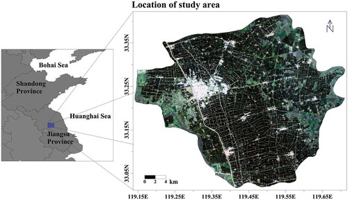
The study area is Baoying xian (similar to county from an administrative perspective), located in central Jiangsu province of China (Figure 1), covering an area of 1467.48 km², approximately 40.1% of which is used for agriculture. This place has a subtropical monsoonal climate, with ample solar illumination and average annual precipitation up to 966 mm, which makes it a great place for crop growth. Baoying has a decent reputation for its organic and high-yield rice, and major crops here include rice, wheat, cotton, and lotus root. Most crop land in this area is used for rice growth in summer and winter wheat during other time, featuring efficient land use from an agronomic perspective.

Figure 1. Location of the study area, Baoying xian, situated at the blue box in left map. For full colour versions of the figures in this paper, please see the online version.

The dominant rice cultivar in Baoying is Huaidao5, constituting almost 83.7% of the total rice planting area. This cultivar features in steady and high yield, with good quality; therefore, its quite popular among local farmers and seed markets. This cultivar belongs to mid-season japonica rice, seeded and transplanted in May and June, respectively, and its harvesting stage ranges from late September to mid-October, depending on weather and irrigation condition.

2.2 Data and preprocessing

Two scenes acquired from Landsat 8 Operational Land Imager (OLI) were collected for this study. Landsat 8 was launched in 11 February 2013, furthering the Earth observation task that had been finished remarkably by its predecessors. It has many advanced technologies for its instruments performance, with main purpose of providing high-quality moderate resolution image data for geoscience research. Compared to the sensor of the last Landsat mission, ETM+, OLI has 12-digit spectral resolution, better signal-to-noise performance, two new spectral bands, and more frequent revisit cycle, enabling it to work well in mapping miscellaneous landscapes. The work presented in this paper is also an attempt to validate the effectiveness of OLI data application on Chinese paddy field mapping.

Although Landsat 8 visits the study area about every twice a month, indicating that at least 10 images can be derived during an approximately 5-month rice-growing cycle, only two images, obtained on 11 August and 27 August, are cloud-free and can be used for this study in 2013 because local rainfall occurs frequently during most part of the rice-growing period. August is an important stage for local paddy growth when paddy is experiencing the transitional phase from vegetative to reproductive growth, thus 2-week difference in data acquisition may contain meaningful cues for rice differentiation from other crops.

The two scenes adopted were carefully preprocessed for three primary steps, which consisted of radiometric calibration, atmospheric correction, and pan-sharpening. The three steps were all successfully completed using ENVI5.0 package. The FLAASH model embedded in ENVI was employed for reliable and fast atmospheric correction before OLI images were radiometrically calibrated into radiance data. The initial visibility parameter required by FLAASH was set to 40 km for the two images, which was tested to be satisfactory for this study. Pan-sharpening was conducted because higher spatial resolution image was better suited for OBIA (Blaschke et al. 2014). Seven multispectral bands with 30-m spatial resolution were pan-sharpened using the panchromatic band (15-m resolution) as input and the Gram–Schmidt (ENVI 2003; Kumar, Sinha, and Taylo 2014) spectral sharpening method to produce multispectral image of 15-m resolution. Nearest neighbor was chosen for resampling because it could preserve the original pixel value of low-resolution bands.

3. Method

3.1 Image segmentation algorithm

Image segmentation is the first step in OBIA. It is defined as a partition of the input image with each region as homogeneous as possible and neighboring ones with sufficiently large heterogeneity. Numerous models have been developed with various extent of success to solve this problem, yet it is still an ongoing issue targeted by many literature to design better methods for different cases. During recent years, some good methods for image segmentation are available in the field of Earth observation, such as FNEA, hierarchical stepwise optimization (HSWO) (Beaulieu and Goldberg 1989), iterative region growing using semantics (Yu and Clausi 2008), mean-shift (Comaniciu 2002), etc.

FNEA, adopting a bottom-up region merging strategy to generate segments, has received much popularity. It is implemented as the multiresolution image segmentation module in the commercial software, eCognition, utilized frequently in studies related to OBIA. FNEA has several advantages. First, it is a hierarchical segmentation method, so differently sized geographic objects can be extracted by simply tuning the scale parameter. Second, FNEA’s merging criterion not only considers spectral properties but also geometric information, thus irregularly shaped ground objects can be extracted with relatively high possibility.

However, this approach has shortcomings sometimes leading to unsatisfactory results that may undermine the subsequent image classification, thus its optimization is justified. On the basis of FNEA, improvements were made in this work, resulting in a new segmentation algorithm including three merging stages (Figure 2). The new method includes two main enhancements: (1) edge and texture information is incorporated into the algorithm to raise segmentation accuracy; and (2) a self-balanced tree structure, combined with the mutual best-fit rule, is utilized to increase running efficiency, at almost no cost on accuracy. The proposed method, combining spectra, shape, edge, texture information, and the hierarchical FNEA, is termed as SETH for convenience.

Figure 2. Working flow of SETH algorithm.

3.1.1 Heterogeneity merge

Similar to FNEA, the first merging stage uses heterogeneity (Baatz and Schaepe 2000) as the merging criterion to perform segmentation starting from an oversegmentation where every pixel is considered as a single segment. The criterion considers spectral and geometric similarity of the candidate adjacent segments to be merged by calculating the heterogeneity change (HC) before and after the merge:

(1)

where ω_shape is a weighting factor in the range of (0,1), balancing the contribution of geometric and spectral information to the total HC. ΔH_spectral and ΔH_shape are spectral HC and shape HC, respectively, and their definitions (Baatz and Schaepe 2000) are as follows:

(2)

(3)

where σ represents spectral standard deviation of the pixels contained in a segment; n means the pixel number of a segment; B is band number; the subscript m symbolizes the segment generated by merging two adjacent segments 1 and 2. ω_compact is also a weighting factor for compactness HC, and ω_compact > 0; ΔH_compact and ΔH_smooth are compactness HC and smoothness HC, respectively, and they are computed by the following equations:

(4)

(5)

where l means the perimeter length (measured in pixel) of a segment; bx represents the length (also measured in pixel) of the bounding box of a segment.

The mutual best fit (MBF) rule (Baatz and Schaepe 2000) is applied to avoid potential erroneous merges. The MBF for two segments (1 and 2) stands if the following conditions are met: (1) the most similar (in this paper, the similarity between two segments is quantitatively measured by Equation (1), with lower value indicating more similar) neighboring segment of 1 is 2; and (2) the most similar neighboring segment of 2 is 1. MBF helps increase segmentation accuracy because some merges of the segments belonging to different geo-object can be avoided by this rule.

All of the segment pairs meeting MBF are ranked according to their HC value (Equation (1)), and the segmentation process starts from merging the most similar pair with the lowest HC. After a merge takes place, the HC scores of the newly merged segment paired with its neighbors are updated. This updating procedure has been emphasized in many FNEA-related researches; however, in our implementation (Figure 3), this operation can be omitted by using MBF and an advanced data structure, which is detailed as follows.

Figure 3. Flow chart of heterogeneity merge implementation.

In order to boost the searching efficiency of FNEA, a data structure, named red-black tree (Cormen et al. 2001), has been employed in our implementation. Red-black tree is a self-balancing binary search tree with good performance for dynamic node inserting, deleting, and searching. Based on a common binary search tree, a red-black tree adds red-or-black color information to its nodes, enabling this data structure to balance its tree depth automatically after an insertion or deletion. So it still works efficiently with temporal complexity of O(log N) (N is node number) in worst scenario when a simple binary search tree degenerates to a linear table. Thanks to the MBF rule, the update of red-black tree is much simplified. Because in the tree construction phase, if MBF is considered, all of the segment pairs are independent, which means that there are no identical segments in different pairs. The newly merged segment in one cycle may be merged with other segment paired with it through tree reconstruction in the following cycle(s) (Figure 3).

The tree reconstruction strategy is more efficient than the traditional updating approach because the latter should be performed every time when a merge occurs, while the former is conducted for each cycle, the merge number of which can be very high in the initial segmentation phase. The process shown in Figure 3 is also used to implement stages 2 and 3, except that the key values used to rank tree nodes are different: at stages 1–3, the key values are HC (Equation (1)), common boundary edge strength (as explained in Section 3.1.2), and a histogram-based criterion (Equation (7)), respectively.

The selection of an appropriate scale parameter is very important at this stage. A large-valued scale threshold may lead to undersegmentation if segments belonging to different ground objects are merged, causing hardly reversible errors at the following stages. In our method, a relatively small threshold T_Het should be set at the first stage to oversegment the image, then the other two stages are performed to further merge the small segments.

3.1.2 Edge merge

The input of this stage is an oversegmentation generated at the first stage. It is usually noticeable that, at the beginning of this stage, large regions are composed of several small segments generally separated by weak boundaries. So edge strength can be used to quickly merge those oversegmented regions. The merging suitability measure at this stage is edge strength value, which is calculated by a vector gradient method, proposed by Lee and Cok (1991).

The method requires two steps to output a single-valued edge strength measure of each pixel for a multiband image. First, differential of Gaussian (DOG) filters of both horizontal and vertical directions are used to obtain edge strength measure for each band, resulting in 2×band gradient maps. Secondly, edge strength for each pixel (i, j) is calculated as the square root of the largest eigenvalue λ_i,_j of matrix D_i,j that is equal to V_i,j·V_i,j^T, where V_i,j is a vector of band×2 dimension, having the following form as Equation (6):

(6)

where and denote the vertical and horizontal DOG filtered result for pixel (i, j) in band k, respectively.

It should be noted that only the two adjacent segments that are mutually found to have the lowest common boundary edge strength among their neighbors are paired for candidate merge. If the edge strength value is larger than a prespecified threshold T_edge, the merge is banned. In practice, a relatively small-valued T_edge is set to avoid undersegmentation, and 50 is used as default by exhaustive experiments.

3.1.3 Merge based on texture described by regional histogram

Texture is important information provided by Earth observation images. But how to use it appropriately is not an easy task. Methods based on gray-level co-occurrence matrix and Gabor filters are two common ways to extract texture information, but they usually suffer from heavy computational cost and may introduce redundant data, which unnecessarily complicates the subsequent analysis, thus they may not be ideal tools for image segmentation that is computation-intensive itself.

Histogram can provide meaningful cues for regional grayscale distribution, and thus it can effectively describe some textural patterns in Landsat images. Yuan, Wang, and Li (2012) presented a segmentation method using local spectral histograms in an attempt to differentiate regions of dissimilar texture in remote sensing images. They concluded that local spectral histogram is an effective way to characterize textural information.

The main purpose of this stage is to merge those adjoining segments with similar texture. At the beginning of this stage, histograms of each segment generated from the last two stages are initialized. Considering computational burden as well as segmentation accuracy, 40 bins for the grayscale ranging from 0 to 255 are determined for segment’s histogram initialization. A criterion, as shown in Equation (3), is designed to quantify the merging suitability of two candidate segments.

(7)

where T_i,j is the textural similarity calculated by two segments’ spectral histograms. N_BIN is the histogram bin number, equal to 40. n_k,i,b is the number of pixel whose grayscale value falls into kth bin of segment i in band b. Segment pair with low value calculated by Equation (7) is considered to be suitable for merge.

The scale parameter T_hist at this stage defines the average size of the resulted segments, so it should be set with much care. A scale selection method described in Section 3.2 was used in our experiment to determine the optimal T_hist for producing the final segmentation result.

3.2 Unsupervised scale selection method for image segmentation

To determine the optimal scale parameter for image segmentation, an unsupervised scale selection method is adopted. This method was first introduced by Johnson and Xie (2011) to optimize the scale selection for fractal net evolution approach. This approach exploits two metrics, area-weighted variance and global Moran’s I, to score a set of scale parameters, from which the optimal one can be selected according to the criterion described as follows.

Considering a set of scale parameters, S = {λ₁, λ₂, …, λ_n}, the score indicating each scale’s goodness for segmentation result is calculated by Equation (8):

(8)

where V_n and M_n are normalized area-weighted variance and global Moran’s I. They are both computed as (X–X_min)/(X_max – X_min), where X can be either area-weighted variance or global Moran’s I, and X_min and X_max are the lowest and highest score derived from the scale set, respectively. Equations (9) and (10) define the area-weighted variance and global Moran’s I, respectively,

(9)

(10)

where n_s is the segment number of a segmentation result produced by a value in the scale parameter set. v_i is the grayscale variance of segment i. w_ij is a weighting factor for segments’ adjacency; it is 1 when segment i and j are neighboring to each other, otherwise it is 0. g_i is the average spectral value for segment i. is the average grayscale value of the whole image.

For a segmentation result of one scale parameter, the V_w and M are recorded for each band, and the GS score of that scale is calculated by V_w and M averaged over all bands. The scale corresponding to the lowest GS among the values derived by a set of scales is chosen as the optimal parameter.

3.3 Object-based feature extraction

Representative object-based features are selected and extracted after segmentation of the input image data. Four major types of segment attributes including geometric, spectral, textural, and contextual information are chosen, with their detailed description listed in Table 1.

Table 1. Object-based features used in this paper.

Feature type	Feature name	Description
Geometric	Area	Segment area, computed as the pixel number of the segment.
	Perimeter	Perimeter length, in unit of pixel.
	Roundness	P^2/A, P is perimeter and A is area. It is small for circular segment, while large for irregularly shaped one.
	Rectangular degree	A/Arect, Arect is the area of the segment’s bounding box. Ranges from 0 to 1, reaches 1 only when the segment is a rectangle.
	Ratio of length and width	The more elongated the segment, the larger value of this feature.
Spectral	Mean (M)	The three features are all calculated for each input band of the bitemporal Landsat images and their NDVI bands.
	Standard deviation (SD)
	Ratio of M and SD
Textural	Gabor filters extracted texture	Gabor filtered result for each spectral band using four spatial and six directional frequencies. Principal component analysis is used for dimension reduction.
Contextual	Mean spectral contrast	The average spectral difference of all neighboring segments for each band.
	Maximal spectral contrast	The maximal spectral difference of all adjacent segments for each band.

As for spectral features, mean, standard deviation, and their ratio of each segment are extracted for the 14 multispectral and 2 normalized difference vegetation index (NDVI) bands of the bitemporal image data set (7 spectral bands plus one NDVI band for each image of one date), resulting in 48 spectral features per segment.

Except spectral features, textural ones are also extracted. Since Gabor filter is a common way to describe texture pattern in remotely sensed images, a bank of Gabor filters with a series of spatial frequencies and orientations are used to convolve the input images. In this study, five spatial frequencies with values of 2√2, 4√2, 8√2, 16√2, and 32√2, and six orientations comprising 0°, 30°, 60°, 90°, 120°, and 150° are tested to be sufficient for texture representation. As a consequence, a total of 420 bands (5 × 6 × 14) of filter responses are obtained, which leads to great computational burden for subsequent processes. Thus, a dimension reduction method based on principal component analysis (PCA) is used. The first seven components with total eigenvalue constitution up to 80.0% are adopted for textural feature extraction. In this way, the processing time of the object-based classification can be largely saved at almost no cost on accuracy.

Additionally, there are two types of contextual features that are designed to respectively delineate mean and maximal spectral contrast between a segment and its neighbors, and are extracted for each spectral and NDVI band, leading to 16 × 2 = 32 contextual features for each segment.

In total, for each segment, its feature vector is composed of 5 + 48 + 7 + 32 = 92 variables, which holds the important information for paddy field recognition. All of the features employed in this paper have been frequently used for agricultural observation by OBIA in other regions (Conrad et al. 2010; Peña-Barragán et al. 2011; Duro, Franklin, and Dubé 2012;).

3.4 Object-based RF classification model

RF was first introduced by Breiman (2001) and frequently used as a supervised machine learning tool for classification and regression problems with remarkable success in many fields. It is designed based on the DT model with improvement in overfitting, prediction accuracy, and the ability to deal with limited training samples. RF contains several DTs, which gives its name “forest.” Ample literature (Duro, Franklin, and Dubé 2012; Zhong et al. 2014; Sonobe et al. 2014) has proved its satisfactory performance in recognition of various geographical objects, including cropped areas (Duro, Franklin, and Dubé 2012; Zheng, Campbell, and Beurs 2012; Sonobe et al. 2014). In this paper, an object-based RF classifier for paddy field classification was implemented and validated.

There are two influential training parameters that should be adjusted with discretion. The first one is maximal tree number (MTN), controlling the uplimit of DTs built during RF training. Large MTN generally leads to good predictability, but it will raise computational burden. After a trial-and-error method, 300 was found to be satisfactory for MTN. The second parameter is the number of variable (NOV), indicating how many attributes are used for a DT node splitting. This parameter, in many studies, was symbolized as m, and empirically set as √P, where P is the dimension of input vector. Although some previous researches (Duro, Franklin, and Dubé 2012; Zhong, Gong, and Biging 2014) claimed that NOV had somewhat effects on training performance, in our experiment it was found to produce little influence on the result and thus was set to 1.

Despite the parameter selection for the RF model, the training strategy also plays a crucial part in the performance of classification. k-fold cross-validation is a standard statistics tool to provide objective training for supervised classifier model (Vieira et al. 2012). This method randomly divides the training samples into k subsets, and each subset is alternatively used for validating the classifier trained by the remaining k–1 sunsets. The process is conducted k times (the folds), and the most accurate model is selected. Larger k value generally results in more objective and robust classifier, but more training samples are needed as k increases. 10 was chosen and tested to be sufficient in our experiment.

3.5 Sample data collection

In order to train and validate the proposed paddy field classification model, 400 samples in total were manually extracted by three experts with reference to high-resolution maps available on Google Earth. Note that each sample was extracted in the form of polygon. All of the samples were stored in a shape file. Since human interpreter may make mistakes in classifying remotely sensed images, the samples were cross-checked by the three experts. A sample was removed if there is one expert having a little doubt for its correctness in the cross-check process. Finally, 383 samples were left and considered to be reliable. Then a stratified random sampling method was adopted to partition the entire sample set into training set and validation set. As a result, there were 97 samples of paddy field and 98 samples of nonpaddy field in the training set, and 96 samples of paddy field and 92 samples of nonpaddy field in the validation set.

4. Results

4.1 Image segmentation validation using subsets

4.1.1 Experiment setup for SETH validation

In order to validate the proposed image segmentation method, two subsets (they will be termed as s1 and s2 for short. s1 refers to the subset image shown in Figure 4(a) and s2 refers to the one displayed in Figure 5(a)) extracted from the OLI image acquired on 27 August with size of 264 × 317 and 353 × 264 pixels, respectively, were used for qualitative and quantitative accuracy assessment. The reasons why subsets were used are twofold. First, the two subsets employed well represented the local landscape of the study area. s1 and s2 both contained various geo-objects, such as rice field, village, road, wetland, and cotton field, so segmentation experiment by using these two subsets can be effective and appropriate. Second, the use of subsets instead of the whole scene was beneficial and convenient for illustration purpose. The detailed visual inspection of the segmentation result of the entire image can be hardly achieved due to too large size.

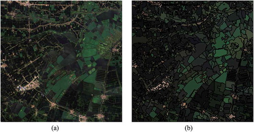
Figure 4. Segmentation results for s1. (a) is the original true color image, (b), (c), (d), and (e) are results of SETH, FNEA, HSWO, and SETH without the third stage, respectively. Note that the colors in (b), (c), (d), and (e) have no special meaning; they are simply formed by averaging the spectral value within each segment.).

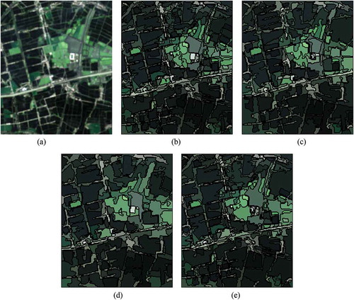
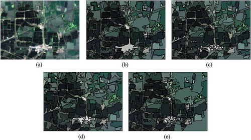
Figure 5. Segmentation results for s2. (a) is the original true color image, (b), (c), (d), and (e) are results of SETH, FNEA, HSWO, and SETH without the third stage, respectively. Note that the colors in (b), (c), (d), and (e) have no special meaning; they are simply formed by averaging the spectral value within each segment.).

Qualitative validation was performed through visual observation and analysis, while the quantitative validation was conducted using three criteria, which were accuracy (ACC) (Fu et al. 2013), m2 measure (Yi, Zhang, and Wu 2012), and correct grouped measure (CG) (Ortiz and Oliver 2006). The three criteria were all supervised evaluation methods, thus manual segmentation by an expert for both s1 and s2 was carefully produced. The definitions of the three metrics are given below:

(11)

(12)

(13)

(14)

(15)

where n_gt is the total number of ground truth segments; |·| indicates cardinality of a set; S_gt represents a set of pixels contained in a ground truth segment, while S_rt symbolizes a set of pixels belonging to a resulted segment; n_gt,_i in Equation (13) means the total number of the resulted segments that are spatially intersected with the ground truth segment S_gt,_i; pr is a threshold and is empirically set as 0.75 (Ortiz and Oliver 2006; Michel, Youssefi, and Grizonnet 2015). This value was tested in this study and turned out to be appropriate. Note that the three criteria all indicate better segmentation result when higher score is achieved and vice versa.

In order to objectively validate the proposed SETH approach, two popular segmentation methods including the traditional FNEA (Baatz and Schaepe 2000) and HSWO (Beaulieu and Goldberg 1989; Tilton et al. 2012) were adopted for comparison because they are both frequently used in OBIA with competitive performance. The traditional FNEA can be considered as a benchmark to test the improvement of the proposed SETH algorithm. The merging criterion of FNEA is HC, as can be seen in Equation (1). HSWO is also a bottom-up region merging method, but it was proposed very early (Beaulieu and Goldberg 1989). Thus, a recently modified version (Tilton et al. 2012) was employed in this work. Compared to the old version, Tilton’s method was improved primarily in two aspects: (1) nonadjacent segments can be considered for merge and (2) running speed of the iterative region merging process is much boosted by a heap-based approach (Williams 1964; Tilton et al. 2012). Note that the merging criterion used in HSWO in this experiment was band sum mean squared error (Tilton et al. 2012).

There are three parameters that need to be tuned for the traditional FNEA: ω_shape, ω_compact, and scale threshold. The former two parameters were set as default as 0.1 and 0.5, respectively. Some related studies indicated that the default values for these two parameters were suitable in most cases (Schultz et al. 2015) and the default setting was tested to be optimal in our experiment. As for HSWO, there are two parameters in total: proximity distance S_w and scale threshold. The former parameter was set to 0 because larger values significantly increased running time and they had trivial influence on segmentation quality in our experiment. As pointed out in Section 3.1, SETH has five parameters to be set: ω_shape, ω_compact, T_Het, T_edge, and T_hist. Note that T_hist is the scale threshold for SETH. To have a fair comparison, ω_shape, ω_compact were set as the same as those for FNEA. Since the purposes of the first and the second stage of SETH are to create oversegmentation, T_Het and T_edge were both set to relatively small values, which were 200 and 100, respectively. Note that the most important parameters for the three algorithms are scale thresholds that should be selected carefully. The unsupervised scale selection approach detailed in Section 3.2 was used for this purpose and this strategy was also beneficial in terms of fair comparison.

4.1.2 Experiment results

The optimal scale parameters for the three segmentation methods were determined via the unsupervised scale selection approach introduced in Section 3.2. Figure 6 illustrates the global scores for a range of scale parameters to be considered for the three segmentation methods, and the scale with the lowest GS was chosen as the optimal scale parameter. Since the scale thresholds for the three methods correspond to different merging criteria, their numerical ranges are different as can be observed on the abscissas of Figure 6.

Figure 6. Scale selection results for the three multiscale segmentation methods. (a), (b), and (c) are results for SETH, FNEA, and HSWO, respectively.

Figures 4 and 5 show the segmentation results produced by the three segmentation algorithms using the optimal scale parameter. Quantitative evaluation scores for s1 and s2, respectively, are tabulated in Tables 2 and 3, with bold figures indicating the best performance among the three methods. Visual comparison also conformed to the quantitative results. Most of the paddy fields were successfully segmented out by SETH, laying an important foundation for the subsequent feature extraction and paddy field classification. It was also obvious by observing s1 and s2 that many adjoining paddy fields were separated by very thin roads, causing weak boundaries between the fields. FNEA and HSWO, whose merging criteria all ignore the edge information, failed to avoid merging those weak-boundary-separated fields, leading to undersegmentation error. Consequently, the ACC, m2, and CG scores for both s1 and s2 were higher for SETH than those of the other two methods, except that for s2, the m2 score of FNEA was slightly better than SETH. Since the difference between the m2 scores of SETH and FNEA for s2 was very small, and the ACC, CG of SETH were all evidently higher than those of FNEA, it can be safely concluded that SETH outperformed FNEA for s2 segmentation.

Table 2. Quantitative validation result of s1.

Method	Optimal scale	ACC	m2	CG
HSWO	3000	0.6386	0.4910	0.5530
FNEA	1700	0.6758	0.4956	0.6465
SETH	0.11	0.8107	0.5194	0.7004
SETH (without the third stage)	200	0.7171	0.4931	0.6550

Note: Bold figures indicating the best performance among the three methods.

Table 3. Quantitative validation result of s2.

Method	Optimal scale	ACC	m2	CG
HSWO	2900	0.5666	0.4277	0.5560
FNEA	1800	0.7175	0.5291	0.5907
SETH	0.13	0.7479	0.4924	0.6417
SETH (without the third stage)	210	0.5944	0.4430	0.5831

Note: Bold figures indicating the best performance among the three methods.

The superior results yielded by the proposed SETH algorithm can be mainly attributed to two reasons. First, three stages utilizing different merging principles were incorporated in SETH, with each stage focusing on different information to find homogeneous segments to be merged, which was more appropriate for semantic merging process. While the other two methods were all constructed on the same criteria throughout the whole merging process, thus they had less chance to produce satisfactory results as compared to our method. Second, more comprehensive information including geometric, spectral, boundary, and textural cues was taken into consideration in the proposed method, so homogeneous segments could be better singled out through this method. FNEA relied on geometric and spectral information to describe the segments’ homogeneity, and HSWO’s merging criterion only considered the spectral information, so relatively poorer results were derived by those two methods.

It is necessary to discuss the effects of the third stage by texture information based on histogram because this stage determines the final average size of the resulted segments for SETH. The segmentation results without the third stage were produced, and the quantitative evaluation scores were calculated for both s1 and s2. The scores are listed in Tables 2 and 3. Note that the scale threshold for SETH without the third stage is T_edge, and this parameter for s1 and s2 was also determined by the unsupervised scale selection approach. As can be seen in Tables 2 and 3, the evaluation scores were all obviously lower than the ones by SETH with the third stage, and visual inspection by Figures 4(e) and 5(e) agreed well with the quantitative evaluation results. This finding proved that the proposed merging criterion of the third stage for SETH was effective for segment texture description, thus erroneous merges can be avoided effectively. It further indicated that texture information is an important factor for segmentation performance, and our method to combine spectra, edge, and texture cues in the proposed merging criteria was successful.

To further test the proposed segmentation approach, another subset, called s3, was used for experiment. s3 was of lower resolution (30 m) because it was not pan-sharpened, thus there were more small fields as compared to s1 and s2. Accordingly, the main purpose of s3 experiment was to validate SETH for more complicated scenarios.

For the sake of saving space, only the result produced by SETH is shown in Figure 7. As can be seen clearly, the average size of crop fields in s3 was almost twice smaller than that in s1 and s2, so lower scale parameter was selected for s3 test, which was 50 and 30 for T_Het and T_edge, respectively. However, the scale parameter of the third merging stage was determined as 0.08, similar to s1 and s2. Quantitative evaluation indicated slightly poorer performance than s1 and s2, with ACC, m2, and CG being 0.6526, 0.5584, and 0.6596, respectively. FNEA and HSWO had quite similar evaluation results, with the three criteria being 0.6133, 0.4667, and 0.5112 for the former and 0.5902, 0.4583, and 0.4847 for the latter method, all lower than the scores of SETH. This further validated the superior performance of SETH.

Figure 7. Segmentation result of s3. (a) is the original image and (b) is the result generated by SETH.

Note that with the scene complexity increasing, the performance of SETH decreased. It can be noticed in Figure 7 that many small paddy fields were merged, resulting in undersegmentation error. This phenomenon could be mainly explained that edge and textural patterns were not very obvious in s3 with lower spatial resolution, so the advantage of the proposed method was not very conspicuous. Moreover, since more types of ground objects were captured in s3, the ground-object size variability and interfield spectral heterogeneity were much higher than those in s1 and s2, leading to greater difficulty in successful segmentation for s3. Thus, the evaluation scores of s3 were relatively lower than those of s1 and s2.

The running time of SETH with and without red-black tree implementation was also compared by using the three subsets, and the results can be found in Table 4. SETH not using red-black tree was implemented by a linear table with O(N) temporal complexity. The computational time of FNEA and HSWO were also given for comparison. Table 4 confirmed the superior running efficiency of the proposed segmentation method since the implementation of SETH using red-black tree was much faster than other approaches. Note that all of the experiments in this paper were performed on a laptop equipped with CPU Intel CORE i5-4200 M (2.50 GHz), 4 GB memory, and Windows 7 operating system (32-bit version).

Table 4. Computational time (in seconds) for the three subsets used in the segmentation experiment.

Data	SETH using red-black tree	SETH not using red-black tree	FNEA	HSWO
s1	1.419	3.298	1.577	3.890
s2	1.326	3.183	1.413	3.776
s3	2.418	5.219	2.556	6.896

4.2 Scale determination for the whole scene

The proposed segmentation algorithm, combined with the unsupervised scale selection method, was applied to the entire image of the study area to automatically produce the segmentation result. Figures 8 and 9 represent the segmentation result and the GS values, respectively. Unlike what is shown in Figure 6, the optimal scale parameter for the whole image segmentation was chosen with more confidence because the optimal scale’s GS was much lower than the other scales in Figure 9, which was not the case in Figure 6. This could be explained by the large size of the whole scene because when calculating the GS for large image segmentation, much more fields were involved, thus more obvious GS goodness of the optimal scale could be observed.

Figure 8. Image segmentation result for the whole scene. The red and blue boxes are the locations of the two subsets to be analyzed in detail.

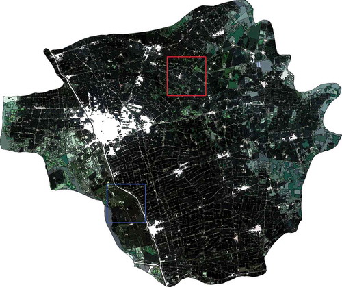
Figure 9. Scale determination result for the segmentation of the whole scene.

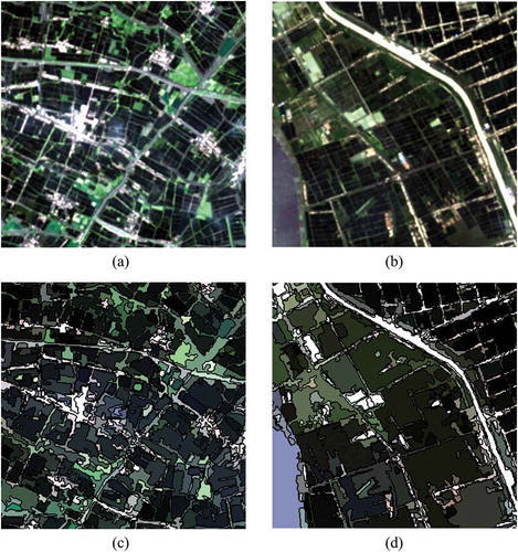
By visually comparing Figure 8 and the original image, it is apparent that most of the homogeneous fields were segmented out with satisfactory performance, despite there existing a few adjacent paddy fields with weak edges inaccurately merged together. Due to the size of the whole image being too large to interpret directly, two subsets with good representativity were chosen and zoomed in for detailed visual inspection. The two sampled subsets are shown in Figure 10, where different characteristics of the two subsets can be evidently observed. As for the left subset in Figure 10, there were many small-sized paddy fields, and a number of them were separated by thin edges. In its segmentation result, although many small paddy fields were merged to form larger ones, this phenomenon was acceptable because those weak edges were too thin to produce significant negative effects on the spectral homogeneity of the resultant segment. Case was more complicated in the right subset, in which large paddy fields with relatively high intra-field variation predominated the image, plus a river and a part of lake bringing more difficulty to its successful segmentation. However, decent segmentation result of the subset, as illustrated in Figure 10(d), further indicated the effectiveness of the proposed method. From the validation works conducted above, it can be safely stated that the proposed segmentation algorithm with the scale selection method was suitable for paddy field extraction by the OBIA approach used in this paper.

Figure 10. Two zoomed-in subsets from the whole scene segmentation result for clear observation and detailed analysis. (a) and (b) are the original subsets corresponding to the red and blue boxes in Figure 8, respectively. (c) and (d) are the segmentation results of (a) and (b), respectively.

4.3 Classification result

After the automatic image segmentation procedure providing the segments to be classified, the object-based RF model was trained using sampled regions/segments, followed by classification to yield the final paddy field thematic map as illustrated in Figure 11. In order to derive the effectiveness of the whole working flow proposed in this paper, the supervised classification evaluation using confusion matrix and kappa statistic (Congalton and Green 2009) was performed.

Figure 11. Final paddy field classification map produced by the object-based RF model.

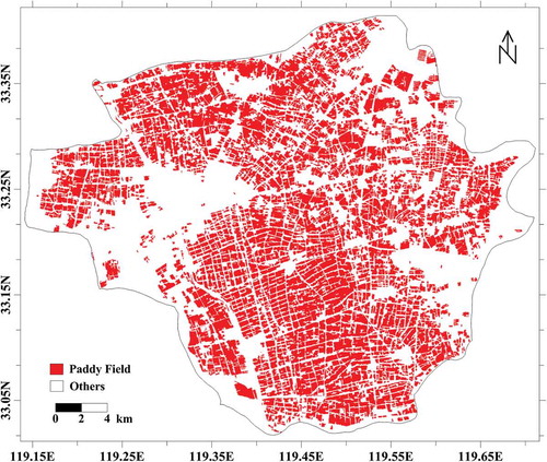
The final classification was conducted by using the bitemporal data set because the data of 11 August and 27 August yielded overall accuracy of 87.28% and 91.02%, respectively, all lower than that of 93.65% produced when the two images were used together. The confusion matrix of the final classification is shown in Table 5, with kappa coefficient of 0.8699, which was quite encouraging and promising since only a bitemporal OLI data set was used.

Table 5. Confusion matrix of the classification result.

	Ground truth
	Result	Paddy field	Other	UA (%)
	Paddy field	84,282	2127	97.54
	Other	11,664	119,034	91.08
	PA (%)	87.84	98.24

Note: Overall accuracy = 93.65%; kappa coefficient = 0.8699.

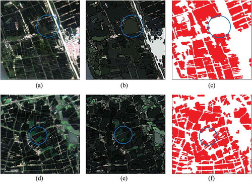
The user’s accuracy (UA) and producer’s accuracy (PA) were also obtained for further analysis. All of the UA and PA for each class were above 87%, which was very satisfactory. However, the paddy field’s PA was comparatively low, indicating that some paddy fields were incorrectly classified as others. A closer examination of the classification map provided the explanation of this error. Since a few small paddy fields were spectrally similar to their neighboring vegetation area, many of them were wrongly merged with its vegetative neighbors in the segmentation step, causing confusion for the RF classifier. Figure 12 shows two examples of this kind of error. This was also observed to be the main source of error for our model. Although the proposed SETH approach can produce more accurate segmentation result, some undersegmentation errors were still hardly avoided, leading to incorrectness for RF classification.

Figure 12. Two examples of the error that paddy fields were erroneously classified as others due to incorrect merge. Blue circles highlight the location of the error. (a) and (d) are original image subsets, (b) and (e) are segmentation results, and (c) and (f) are classification results with legend similar to that of Figure 11.

It can be also observed that in the classification result most paddy fields were well separated from other wetlands. This was largely attributed to the acquisition date of OLI data because in August paddy fields were mostly covered by vegetation, thus wetlands such as water ponds and shallow rivers were spectrally different from paddy fields.

The total paddy field area was computed by using the final classification map to further support the reliability of the classification result. First, the pixels classified as paddy were counted and then the pixel number was multiplied by the area of each pixel to derive the final paddy area estimation, which amounted to 59,802 ha. This result was compared to the official statistic, which was 58,353 ha, provided by the Baoying xian government in 2013. The two figures were in close agreement, with relative difference of only 2.48%, which further justified the performance of the proposed method. The reason why the estimated paddy field area by classification map was slightly higher than the official record can be largely ascribed to the undersegmentation error resulting from merging paddy fields spaced by weak boundary. Although a pixel-based classification method may simply avoid this type of error, considering the correctness of the area estimated by our OBIA method, the good validation result still held water.

4.4 Feature importance

One merit of RF model is that it can quantify the relative contribution for each input feature used for classifier training, thus providing meaningful clues for users to understand the importance of each feature, and thus offering important reference for related studies.

In RF classification algorithm, importance score (IS) of each feature was calculated right after its training when all of the DTs in RF were constructed through an out-of-bag procedure (Breiman 2001). Rises in prediction error were estimated for each feature variable, which was used as a single input to run the trained RF. The feature with the lowest error increase was considered to carry the most predictive information, and thus having the highest IS value.

As clearly illustrated by Figure 13, each feature’s IS can be observed. It is obvious to note that spectral features contributed the most among the four feature types. Textural and contextual features also made some contribution to the classifier, but geometric information was the least useful feature type.

Figure 13. Feature importance for each feature variable considered in the RF model. From left to right, the feature order is: geometric features: area, perimeter, roundness, rectangular degree, ratio of width and length; spectral features: for each band, mean (M), standard deviation (SD), ratio of mean and standard deviation (R) of the segment are in the order of M₁₁, SD₁₁, R₁₁, M₂₁, SD₂₁, R₂₁, …, Mij, SDij, Rij, …, where i represents the band number, ranging from 0 to 7, with 0 being the NDVI, 1 the coastal aerosol band (443 nm), 2 the blue band (483 nm), 3 the green band (516 nm), 4 the red band (655 nm), 5 the near infrared (NIR) band (865 nm), 6 the short wave infrared (SWIR) 1 band (1609 nm), and 7 the SWIR2 band (2201 nm), j indicates data date, with 1 representing 11 August and 2 representing 27 August; textural features: seven Gabor filtered bands transformed through PCA and ranked according to their eigenvalue; contextual features: for each band, mean spectral contrast (MSC) and maximal spectral contrast (MASC) are in the order of MSCij, MASCij, with i and j having the same definition for the spectral features.

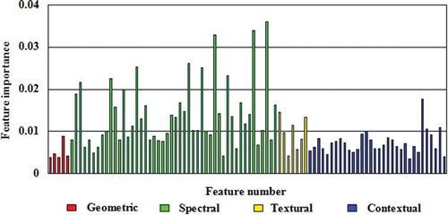
The best geometric feature was rectangular degree, with almost one time higher IS than the other four geometric variables. In the study area, most rice planting fields were rectangular shaped, which may be the main cause of this fact. But this feature’s IS still ranked much lower than the other types of features, which may be explained by the fact that some other land covers, that is, water pools, cotton fields, and garden lawns, had high rectangular degree.

Contrary to geometric features, spectral features were much more important. Although the two OLI scenes used in this study were only 2 weeks away, they contained key information for paddy fields recognition, which can be confirmed by their high IS. Moreover, it can be observed from Figure 13 that the spectral features extracted from 11 August data were less important than the counterparts of 27 August. The three variables with the highest IS all belong to spectral feature type, and they were all mean spectral variables. According to IS, the three most important mean spectral features were SWIR2, SWIR1, and green band, all acquired from 27 August. As for each spectral band with relatively high IS score, the IS of mean spectral value was higher than the other two spectral features, except NDVI band, with mean value being the least important among the three spectral features. This may be resulted from that the duration of the bitemporal OLI data was relatively short, thus NDVI mainly representing vegetation biomass can hardly provide any crucial information on paddy fields classification; by contrast, the data acquisition time was at the intensive growing stage of paddy, during which the spectral responses of certain bands may appear to be different.

On the other hand, the contribution of textural features was much lower as compared to spectral ones. However, it is still interesting to note that the IS of the spectral textural were not in line with their eigenvalues derived from PCA. The component with the lowest eigenvalue had the second highest IS. So when using textural features to classify paddy fields, special attention must be made in the feature selection to raise the classification performance.

As for contextual features, most variables were of low IS, except that the mean spectral contrast (MSC) of near infrared (NIR) band, obtained from 27 August, contributed significantly higher than other contextual features. However, the contribution of this band’s spectral features was not so distinct. So it can be inferred that the NIR band was somewhat useful to differentiate the neighboring ground objects from paddy fields in the study area.

In summary, spectral features were the most influential in this study, and they were in turn recommended for other related researches. Aside from spectral features, an NIR band feature belonging to contextual type had distinctively high IS, which supported the usefulness of OBIA. Geometric and textural information should be used with discretion since in our experiment the IS of the two feature types was not very significant.

5. Discussion

The main contribution of this work is the newly established SETH segmentation approach. Validation experiment indicated the superior segmentation accuracy of SETH. This is mainly attributed to the proposed merging criteria, which fully utilized spectral, geometric, edge, and textural information. However, there is one issue worth mentioning. This study only adopted Landsat-8 OLI images with 15 m spatial resolution. Since SETH is based on FNEA, which has been widely used for handling high spatial resolution images, the mapping accuracy of the proposed framework may not be optimal. However, we argue that this issue is not significant. The reasons are stated as follows.

As pointed out by Blaschke et al. (2014), OBIA is well applicable to the interpretation of high-resolution data, but this kind of technique is not limited to high-resolution images. If the interested geo-objects have relatively large area in medium and coarse resolution data, then OBIA is also feasible. For example, Vieira et al. (2012) used OBIA to map sugarcane in Brazil. The data adopted in their study were Landsat TM and ETM+ images with spatial resolution of 30 m. Peña-Barragán et al. (2011) also used OBIA and 15 m medium resolution data acquired by ASTER to map crop types. Both of these studies employed FNEA (in their papers, FNEA was referred to as the multiresolution segmentation approach) as the segmentation strategy, and good classification results were derived. In our study, paddy fields have relatively large area as compared to the pixel size of Landsat-8 images, which can be observed in Figures 4(a), 5(a), 7(a), and 10(a) and (b). Accordingly, it is reasonable to exploit 15 m resolution image to classify paddy fields by the proposed OBIA framework.

6. Conclusion

This paper aimed at establishing an OBIA framework for paddy fields mapping, which comprised four components including a novel three-stage image segmentation method, a fully automatic and unsupervised scale selection approach, an object-based feature extraction, and an object-based RF classifier. The proposed methodology was tested by using a bitemporal data set acquired by Landsat-8 over Baoying xian, and the mapping accuracy was quite satisfactory according to the quantitative evaluation scores. The main contributions of this paper are summarized as follows.

First, a new image segmentation algorithm, constructed on the basis of FNEA with enhancement primarily in merging criteria, was proposed. Quantitative evaluation indicated that the proposed segmentation enhanced accuracy. The running efficiency of the proposed SETH algorithm was also increased due to the adoption of red-black tree structure that optimized the implementation. Second, unlike other OBIA researches, a fully unsupervised scale selection method was combined with the proposed image segmentation, so users did not have to tune the scale parameter through the time-consuming trial-and-error method, significantly increasing the automation and objectivity of the whole data processing chain. Third, an object-based RF classifier, which was tested to produce accurate paddy field classification, yielded the relative contribution of each object-based feature, helping users understand the feature importance. Last but not least, although only a bitemporal OLI data set was exploited in this work, the effectiveness derived by our OBIA framework surely justified its feasibility, and it at least indicated that, in some regions like Baoying xian, only a few scenes of mediate resolution data captured during the intensive cropping stage can be sufficient for paddy field classification.

From the aforementioned contributions of this study, two implications were found to be meaningful for future works. First, the proposed SETH algorithm can be extended to other OBIA-based classification tasks. Due to the superior segmentation evaluation scores of SETH, it is worth expecting that the proposed segmentation method has good performance for other OBIA applications, such as building classification, road recognition, and forest mapping. Second, it is encouraging that good classification accuracy can be achieved by using only a bitemporal data set. Due to the fact that rice growth period is accompanied by monsoonal climate, remotely sensed images by optical sensors are often contaminated by cloud cover, thus many data cannot be used during one crop cycle. Thus, the result of this paper supports the feasibility of accurate paddy field classification by using very few images. This finding actually encourages the operational use of paddy field mapping by Landsat-8 OLI and other similar optical satellite sensors.

Acknowledgments

USGS is sincerely thanked for their generosity of data provision. The work presented in this paper was partly supported by National Natural Science Foundation under grant [number 51569017 and 51569018].

Disclosure statement

No potential conflict of interest was reported by the author.

Additional information

Funding

The work presented in this paper was partly supported by National Natural Science Foundation under grant [number 51569017 and 51569018].

References

- Amorós-López, J., L. Gómez-Chova, L. Alonsoa, L. Guanterb, R. Zurita-Millac, J. Morenoa, and G. Camps-Valls. 2013. “Multi-Temporal Fusion of Landsat/TM and ENVISAT/MERIS for Crop Monitoring.” International Journal of Applied Earth Observation and Geoinformation 23: 132–141. doi:10.1016/j.jag.2012.12.004.
- Baatz, M., and A. Schaepe. 2000. “Multiresolution Segmentation: An Optimization Approach for High Quality Multi-Scale Image Segmentation.” Angewandte Geographische Informationsverarbeitung 7: 12–23.
- Beaulieu, J., and M. Goldberg. 1989. “Hierarchy in Picture Segmentation: A Step-Wise Optimization Approach.” IEEE Transactions on Pattern Analysis and Machine Intelligence 11: 150–163. doi:10.1109/34.16711.
- Blaschke, T. 2010. “Object Based Image Analysis for Remote Sensing.” ISPRS Journal of Photogrammetry and Remote Sensing 65 (1): 2–16. doi:10.1016/j.isprsjprs.2009.06.004.
- Blaschke, T., G. J. Hay, M. Kelly, S. Lang, P. Hofmann, E. Addink, R. Q. Feitosa, et al. 2014. “Geographic Object-Based Image Analysis - Towards a New Paradigm.” ISPRS Journal of Photogrammetry and Remote Sensing 87: 180–191. doi:10.1016/j.isprsjprs.2013.09.014.
- Breiman, L. 2001. “Random Forests.” Machine Learning 45 (1): 5–32. doi:10.1023/A:1010933404324.
- Comaniciu, D. 2002. “Mean Shift: A Robust Approach toward Feature Space Analysis.” IEEE Transactions on Pattern Analysis and Machine Intelligence 24 (5): 603–619. doi:10.1109/34.1000236.
- Congalton, R. G., and K. Green. 2009. Assessing the Accuracy of Remotely Sensed Data: Principles and Practices. 2nd ed. London: CRC Press.
- Conrad, C., S. Fritsch, J. Zeidler, G. Rücker, and S. Dech. 2010. “Per-Field Irrigated Crop Classification in Arid Central Asia Using SPOT and ASTER Data.” Remote Sensing 2: 1035–1056. doi:10.3390/rs2041035.
- Cormen, T. H., E. L. Charles, R. L. Rivest, and C. Stein. 2001. Introduction to Algorithms, 238p. 2nd ed. London: The MIT Press.
- Dong, J., X. Xiao, M. A. Menarguez, G. Zhang, Y. Qin, D. Thau, C. Biradar, and B. Berrien Moore. 2016. “Mapping Paddy Rice Planting Area in Northeastern Asia with Landsat 8 Images, Phenology-Based Algorithm and Google Earth Engine.” Remote Sensing of Environment 185: 142–154. doi:10.1016/j.rse.2016.02.016.
- Duro, D. C., S. E. Franklin, and M. G. Dubé. 2012. “A Comparison of Pixel-Based and Object-Based Image Analysis with Selected Machine Learning Algorithms for the Classification of Agricultural Landscapes Using Spot-5 HRG Imagery.” Remote Sensing of Environment 118: 259–272. doi:10.1016/j.rse.2011.11.020.
- ENVI. 2003. ENVI Users Guide, Version 4.0, 1084. Research Systems. Colarado: Boulder.
- Fu, G., H. Zhao, C. Li, and L. Shi. 2013. “Segmentation for High-Resolution Optical Remote Sensing Imagery Using Improved Quadtree and Region Adjacency Graph Technique.” Remote Sensing 5: 3259–3279. doi:10.3390/rs5073259.
- Gumma, M. K., A. Nelson, P. Thenkabail, and A. Singh. 2011. “Mapping Rice Areas of South Asia Using MODIS Multi-Temporal Data.” Journal of Applied Remote Sensing 5: 1–26. doi:10.1117/1.3619838.
- Hadria, R., B. Duchemin, L. Jarlan, G. Dedieu, F. Baup, S. Khabba, A. Olioso, and T. L. Toan. 2010. “Potentiality of Optical and Radar Satellite Data at High Spatio-Temporal Resolutions for the Monitoring of Irrigated Wheat Crops in Morocco.” International Journal of Applied Earth Observation and Geoinformation 12: 32–37. doi:10.1016/j.jag.2009.09.003.
- Johnson, B., and Z. Xie. 2011. “Unsupervised Image Segmentation Evaluation and Refinement Using a Multi-Scale Approach.” ISPRS Journal of Photogrammetry and Remote Sensing 66: 473–483. doi:10.1016/j.isprsjprs.2011.02.006.
- Kim, H., and J. Yeom. 2014. “Effect of Red-Edge and Texture Features for Object-Based Paddy Rice Crop Classification Using Rapideye Multi-Spectral Satellite Image Data.” International Journal of Remote Sensing 35: 7046–7068.
- Kobayashi, T., E. Kanda, K. Ishiguro, and Y. Torigoe. 2001. “Detection of Rice Panicle Blast with Multispectral Radiometer and the Potential of Using Airborne Multispectral Scanners.” The American Phytopathological Society 91: 316–323. doi:10.1094/PHYTO.2001.91.3.316.
- Kuenzer, C., and K. Knauer. 2013. “Remote Sensing of Rice Crop Areas.” International Journal of Remote Sensing 34: 2101–2139. doi:10.1080/01431161.2012.738946.
- Kumar, L., P. Sinha, and S. Taylo. 2014. “Improving Image Classification in a Complex Wetland Ecosystem through Image Fusion Techniques.” Journal of Applied Remote Sensing 8: 1–16. doi:10.1117/1.JRS.8.083616.
- Laliberte, A. S., A. Rango, K. M. Havstad, J. F. Paris, R. F. Beck, R. McNeely, and A. L. Gonzalez. 2004. “Object-Oriented Image Analysis for Mapping Shrub Encroachment from 1937 to 2003 in Southern New Mexico.” Remote Sensing of Environment 93: 198–210. doi:10.1016/j.rse.2004.07.011.
- Lee, H.-C., and D. R. Cok. 1991. “Detecting Boundaries in a Vector Field.” IEEE Transactions on Signal Processing 39: 1181–1194. doi:10.1109/78.80971.
- Lyons, M. B., S. R. Phinn, and C. M. Roelfsema. 2012. “Long Term Land Cover and Seagrass Mapping Using Landsat and Object-Based Image Analysis from 1972 to 2010 in the Coastal Environment of South East Queensland, Australia.” ISPRS Journal of Photogrammetry and Remote Sensing 71: 34–46. doi:10.1016/j.isprsjprs.2012.05.002.
- Michel, J., D. Youssefi, and M. Grizonnet. 2015. “Stable Mean-Shift Algorithm and Its Application to the Segmentation of Arbitrarily Large Remote Sensing Images.” IEEE Transactions on Geoscience and Remote Sensing 53: 952–964. doi:10.1109/TGRS.2014.2330857.
- National Bureau of Statistics of China. 2015. “The Bulletin on Crop Yield of Year 2014 from National Bureau of Statistics of China.” National Bureau of Statistics of China. December 4. Accessed 4 January 2015. http://www.stats.gov.cn/tjsj/zxfb/201412/t20141204_648275.html. (in Chinese).
- Nguyen-Thanh, S., C. Chen, C. Chen, H. Duc, and L. Chang. 2014. “A Phenology-Based Classification of Time-Series MODIS Data for Rice Crop Monitoring in Mekong Delta, Vietnam.” Remote Sensing 6: 135–156.
- Ortiz, A., and G. Oliver 2006. “On the use of the overlapping area matrix for imagesegmentation evaluation: A survey and new performance measures.” Pattern Recognition Letters 27: 1916–1926. doi:10.1016/j.patrec.2006.05.002
- Panigrahy, S., and S. A. Sharma. 1997. “Mapping of Crop Rotation Using Multidate Indian Remote Sensing Satellite Digital Data.” ISPRS Journal of Photogrammetry and Remote Sensing 52: 85–91. doi:10.1016/S0924-2716(97)83003-1.
- Peña-Barragán, J. M., P. A. Gutiérrez, C. H. Martínez, J. Six, R. E. Plant, and F. L. Granados. 2014. “Object-Based Image Classification of Summer Crops with Machine Learning Methods.” Remote Sensing 6: 5019–5041. doi:10.3390/rs6065019.
- Peña-Barragán, J. M., M. Ngugi, R. E. Plant, and J. Six. 2011. “Object-Based Crop Identification Using Multiple Vegetation Indices, Textural Features and Crop Phenology.” Remote Sensing of Environment 115: 1301–1316. doi:10.1016/j.rse.2011.01.009.
- Sakamoto, T., B. D. Wardlow, A. A. Gitelson, S. B. Verma, A. E. Suyker, and T. J. Arkebauer. 2010. “A Two-Step Filtering Approach for Detecting Maize and Soybean Phenology with Time-Series MODIS Data.” Remote Sensing of Environment 114: 2146–2159. doi:10.1016/j.rse.2010.04.019.
- Schultz, B., M. Immitzer, A. R. Formaggio, I. D. A. Sanches, A. J. B. Luiz, and C. Atzberger. 2015. “Self-Guided Segmentation and Classification of Multi-Temporal Landsat 8 Images for Crop Type Mapping in Southeastern Brazil.” Remote Sensing 7: 14482–14508. doi:10.3390/rs71114482.
- Shen, S. H., S. B. Yang, B. B. Li, B. X. Tan, Z. Y. Li, and T. L. Toan. 2009. “A Scheme for Regional Rice Yield Estimation Using ENVISAT ASAR Data.” Science in China Series D: Earth Sciences 52: 1138–1194.
- Sonobe, R., H. Tani, X. Wang, N. Kobayashi, and H. Shimamura. 2014. “Random Forest Classification of Crop Type Using Multi-Temporal Terrasar-X Dual-Polarimetric Data.” Remote Sensing Letters 5: 157–164. doi:10.1080/2150704X.2014.889863.
- Tilton, J. C., Y. Tarabalka, P. M. Montesano, and E. Gofman. 2012. “Best Merge Region-Growing Segmentation with Integrated Nonadjacent Region Object Aggregation.” IEEE Transactions on Geoscience and Remote Sensing 50: 4454–4467. doi:10.1109/TGRS.2012.2190079.
- Valipour, M. 2014. “Future of Agricultural Water Management in Africa.” Archives of Agronomy and Soil Science 61: 907–927. doi:10.1080/03650340.2014.961433.
- Valipour, M. 2015. “Land Use Policy and Agricultural Water Management of the Previous Half of Century in Africa.” Applied Water Science 5: 367–395. doi:10.1007/s13201-014-0199-1.
- Valipour, M., M. Z. Ahmadi, M. Raeini-Sarjaz, M. A. G. Sefidkouhi, A. Shahnazari, R. Fazlola, and A. Darzi-Naftchali. 2014. “Agricultural Water Management in the World during past Half Century.” Archives of Agronomy and Soil Science 61: 1–22.
- Vieira, M. A., A. R. Formaggio, C. D. Rennó, C. Atzberger, D. A. Aguiar, and M. P. Mello. 2012. “Object Based Image Analysis and Data Mining Applied to a Remotely Sensed Landsat Time-Series to Map Sugarcane over Large Areas.” Remote Sensing of Environment 123: 553–562. doi:10.1016/j.rse.2012.04.011.
- Wang, C., J. Wu, Y. Zhang, G. Pan, J. Qi, and W. A. Salas. 2009. “Characterizing L-Band Scattering of Paddy Rice in Southeast China with Radiative Transfer Model and Multi-Temporal ALOS/PALSAR Imagery.” IEEE Transactions on Geoscience and Remote Sensing 47: 988–998. doi:10.1109/TGRS.2008.2008309.
- Williams, J. W. J. 1964. “Heapsort.” Communications of the ACM 7: 347–348.
- Wu, F., C. Wang, H. Zhang, B. Zhang, and Y. Tang. 2011. “Rice Crop Monitoring in South China with RADARSAT-2 Quad-Polarization SAR Data.” IEEE Geoscience and Remote Sensing Letters 8: 196–200. doi:10.1109/LGRS.2010.2055830.
- Yang, S., S. Shen, B. Li, T. L. Toan, and W. He. 2008. “Rice Mapping and Monitoring Using ENVISAT ASAR Data.” IEEE Geoscience and Remote Sensing Letters 5: 108–112. doi:10.1109/LGRS.2007.912089.
- Yi, L., G. Zhang, and Z. Wu. 2012. “A Scale-Synthesis Method for High Spatial Resolution Remote Sensing Image Segmentation.” IEEE Transactions on Geoscience and Remote Sensing 50: 4062–4070. doi:10.1109/TGRS.2012.2187789.
- Yu, Q., and D. A. Clausi. 2008. “IRGS: Image Segmentation Using Edge Penalties and Region Growing.” IEEE Transactions on Pattern Analysis and Machine Intelligence 30 (12): 2126–2139. doi:10.1109/TPAMI.2008.15.
- Yuan, J., D. Wang, and R. Li. 2012. “Image Segmentation Using Local Spectral Histograms and Linear Regression.” Pattern Recognition Letters 33: 615–622. doi:10.1016/j.patrec.2011.12.003.
- Zheng, B., J. B. Campbell, and K. M. D. Beurs. 2012. “Remote Sensing of Crop Residue Cover Using Multi-Temporal Landsat Imagery.” Remote Sensing of Environment 117: 177–183. doi:10.1016/j.rse.2011.09.016.
- Zhong, L., P. Gong, and G. S. Biging. 2014. “Efficient Corn and Soybean Mapping with Temporal Extendability: A Multi-Year Experiment Using Landsat Imagery.” Remote Sensing of Environment 140: 1–13. doi:10.1016/j.rse.2013.08.023.