Using satellite-based soil moisture to detect and monitor spatiotemporal traces of agricultural drought over Bundelkhand region of India

Abstract

Detection and monitoring of seasonal agricultural drought at sub-regional scale is a complex theme due to inefficient spatiotemporal indicators. This study presents a new time-based function of spaceborne soil moisture as an efficient indicator. Bundelkhand of Central India, a frequently agricultural drought affected region, was used as the study area. Rabi agricultural season (October–May) being the dominant agricultural return period, was chosen as the study period. Coarse resolution soil moisture (SM_c) obtained from European space agency under climate change initiative program was spatially downscaled (SM_d) to meet spatial scale at sub-regional level with overall root-mean-square error under 0.065 cm³/cm³. Indirect validation of SM_d was done using temporal impact of rainfall/dry spell on SM_d and spatiotemporal impact of SM_d on vegetation condition. SM_d was found to agree with phenomenon as expected in natural processes and hence it was assumed to be validated. The time-based function derived from spatiotemporal SM_d (FSM_s) was found to be better related with fluctuations in seasonal crop yield (Y_s) at district level as compared to a similar function (FVCI_s) derived using vegetation condition index (VCI) from Moderate Resolution Imaging Spectroradiometer. FSM_s outperformed FVCI_s having better correlation coefficient (R ≥0.8) and Nash–Sutcliffe efficiency coefficient (NSE) than FVCI_s for most of the districts. Unlike FVCI_s, it also efficiently detected the lowest and highest Y_s for majority of the districts representing better association with agricultural drought. Subsequently, frequent soil moisture deficit areas were mapped by using FSM_s to visualize the spatiotemporal severity of agricultural drought in the region during Rabi season.

Keywords:

• satellite soil moisture
• agricultural drought
• spatial downscaling
• effective drought index (EDI)
• vegetation condition index (VCI)

1. Introduction

There are several ways of monitoring drought but it gets complex when monitoring for fields of its impact. Agricultural drought is one of such fields, which are classified as calamity that can affect economy and society at regional to national extents (Wilhite 2000). It is a serious issue faced time to time in India since long back (Aggarwal 2008). There could be many reasons for agricultural drought occurrence such as untimed/insufficient irrigation, untimed/scarce rainfall, improper management, over/under dose in application of fertilizers, low yield variety of crops, etc. (Rockström and Falkenmark 2000; Shinde and Modak 2013). Various indicators have been utilized by the researchers to monitor agricultural drought relating to the reason of occurrence such as time series observation of meteorological and hydrological parameters. Indicators derived from meteorological observations are helpful in rain-fed agriculture, whereas irrigated agriculture require indicators from both meteorological and hydrological observations (Rockström, Barron, and Fox 2002). These observations are from point sources which are best for temporal monitoring at point location but fails in spatial dimension. Moreover, the quantity and time of application of water from sources of irrigation like rainwater, groundwater, canal, and storage tanks vary in spatial dimension with variable management schemes as well. Utility of meteorological and hydrological parameters with good spatial results at vast region demands dense distribution of observation points which is difficult to attain. Recent advancements in remote sensing technology have provided new directions in agricultural drought monitoring (Thenkabail, Gamage, and Smakhtin 2004; Senay et al. 2015; Wu, Qu, and Hao 2015). Reflectance from ground recorded by the satellites is used to derive indices which represent plant health. Remote sensing techniques might not be as good as meteorological and hydrological indicators at a point scale, but serves best for spatial extents with reasonable temporal details. The success of indices derived from satellite data was so extraordinary that it is being used at operational level for national and global drought monitoring (Seshasai et al. 2016; Zhang et al. 2017). However, thematic subjects such as detection and monitoring of seasonal agricultural drought are complex and demands support from different indicators and efficient methodologies.

Agricultural drought refers to a period with declining soil moisture content and consequent crop failure from water stress (Mishra and Singh 2010). Water stress has been proved to be a major cause for occurrence of agricultural drought in various studies (Narasimhan and Srinivasan 2005; Farooq et al. 2009; Gago et al. 2015; Pérez-Blanco et al. 2016). Soil moisture is believed to be one of the significant indicators of water stress and hence agricultural drought (Bolten et al. 2010; Mao et al. 2017). Soil moisture shows the capability to explain the aftereffects of rainfall/dry spell, evapotranspiration and any kind of irrigation. Being interactive at root zone of crops, soil moisture is physically related to growth and health of crops at the same time (Boken, Cracknell, and Heathcote 2005; Wilhite 2005; Holzman, Rivas, and Piccolo 2014). Therefore, monitoring the soil hydrology is anticipated to expose spatiotemporal occurrence of agricultural drought. However, researchers around the world face problems in using direct measurement of soil moisture for such studies due to difficulty in obtaining densely distributed in situ measurements in developing countries like India. As an alternative, microwave remote sensing had shown its potential since last three decades to estimate geophysical parameters such as soil moisture using properties of backscatter and brightness temperature (Kondratyev et al. 1977; Njoku and Entekhabi 1996; Du, Ulaby, and Dobson 2000; Guha and Lakshmi 2004). Nowadays soil moisture is estimated operationally using active or passive microwave remote sensing. Soil moisture retrieved from active microwave remote sensing data such as European Remote Sensing Satellite Scatterometer (ERS-SCAT), Advanced Scatterometer (ASCAT), etc., are good in spatial resolution, but it is an expensive source with poor spatial coverage and temporal resolution. Whereas passive microwave-derived soil moisture from sources such as soil moisture ocean salinity (SMOS), advanced microwave scanning radiometers (AMSR-E, AMSR2), and soil moisture active passive (SMAP) are inexpensive and good in spatial coverage, but deals with issues like coarse spatial resolution. Knowing the importance of soil moisture, it was recognized as an essential climatic variable by European Space Agency (ESA) and a blended spatial soil moisture product from several successful active and passive microwave remote sensing sources was released under climate change initiative (CCI) in 2010. It is available at daily interval with resolved temporal issues and has been encouraged to assimilate with satellite-derived data sets (Reichle et al. 2004). This blended product has been used successfully in several drought-related studies (Anderson et al. 2012; McNally et al. 2016; Rahmani, Golian, and Brocca 2016).

The present research explores geospatial data, that is, soil moisture from CCI, ESA, and Moderate Resolution Imaging Spectroradiometer (MODIS) products, precipitation records and seasonal crop yield data with an objective of utilizing the spatiotemporal behavior of soil moisture in seasonal agricultural drought monitoring. Soil moisture at coarse resolution (SM_c) was spatially downscaled using triangle method (Carlson 2007) to meet the requirement of spatial resolution at sub-regional/district level. The downscaled soil moisture (SM_d) was validated for its statistical significance with SM_c. It was also validated for its dependency on meteorological events by using effective drought index (EDI) as meteorological parameter and an influencing factor for consequential condition of vegetation by using vegetation condition index (VCI). EDI was computed from rainfall data collected from several stations in the study area as shown by Byun and Wilhite (1999) and used to validate dependency of SM_d on rainfall/dry spells. Again, VCI (Kogan 1990) is a popular widely used remote sensing index used in agricultural drought studies (Quiring and Ganesh 2010; Rhee, Im, and Carbone 2010; Jiao et al. 2016), which was derived from MODIS normalized difference vegetation index (NDVI) and used to validate the SM_d as a factor of influence on vegetation condition. The limitation of unavailability of in situ soil moisture data was thus overcome by validating SM_d using the indicators exhibiting the relationship with soil moisture agreeing with natural processes (e.g. rainfall/day spell and vegetation condition). A unique method based on the crop phenology was used to target only seasonal agricultural areas for spatiotemporal agricultural drought monitoring. Finally, time-based function of SM_d and VCI derived from MODIS NDVI were utilized to detect the trends in seasonal crop yield (Y_s), this attempt highlights the strength of the remote sensing-derived soil moisture as an efficient indicator for monitoring seasonal agricultural drought. The methodology used in this study has the potential to trace seasonal agricultural drought in spatiotemporal dimensions at sub-regional scale by using soil moisture from various past and present satellite sources in arid/semi-arid regions.

2. Study area

Bundelkhand region of India is located at latitude ranging from 23°10ʹ N to 26°27ʹ N and longitude from 78°40ʹ E to 81°34ʹ E (Figure 1). The total area of this region is around 30,000 km². It includes 13 districts in states of Uttar Pradesh (Jhansi, Jalaun, Lalitpur, Hamirpur, Mahoba, Banda, and Chitrakoot) and Madhya Pradesh (Datia, Tikamgarh, Chattarpur, Damoh, Sagar, and Panna). The climate of this region is semi-arid with minimum and maximum temperatures ranging from 6–12°C to 38–48°C, respectively. The post-monsoon or Rabi season (October–May) is the primary agricultural season for Bundelkhand region as the agricultural returns gained in this season is highest in a year. The main crops in Rabi season are Wheat and Gram which together covers more than 90% of total Rabi crop acreage. A larger part of the agriculture in Bundelkhand region is rain-fed as compared to irrigated practice, with evenly distributed mixed practices for water supply over both the states. These areas have water supply either from minor irrigation systems like groundwater, tanks, small reservoirs, etc., or precipitation water depending on the occurrence. However, ground water is the largest source of water supply for Rabi agriculture after rain-fed practice in the study area. The minor rainfall events occur during the month of January and February due to Western disturbances. The occurrence of these trivial events is important for the Rabi season as the agriculture of a large part in the Bundelkhand region depends on it. The population of Bundelkhand region is approximately 50 million out of which 80% population rely on agriculture. Bundelkhand region is a frequently drought affected zone (Patel and Yadav 2015). The frequency of drought has gradually increased in this region, the drought occurrence frequency has tripled in recent times as compared to condition prior to year 1968 (Singh, Roy, and Kogan 2003). The region has experienced drought every year since 2004–2005 (NRAA 2008). As a result, various sectors of the region including the agriculture are accounted to suffer heavily in the past decade.

Figure 1. Geographical extent of Bundelkhand region and its districts.

3. Materials and methods

3.1. Data description

The datasets were obtained from various sources for varying timespans and indicators were derived from it. However, this work is focused on the spatiotemporal agricultural drought detection in Rabi agricultural season, due to which a common timespan (October–May, 2003–2004 to 2008–2009) was selected for the study as per the availability of all data.

3.1.1. Satellite soil moisture

The basic soil moisture data used for the study is global soil moisture available under CCI from website of ESA (http://www.esa-soilmoisture-cci.org). This dataset was generated by blending soil moisture products derived from space borne active and passive microwave instruments (Liu et al. 2011, 2012; Wagner et al. 2012). The active dataset was generated by the Vienna University of Vienna (TU Wien) using the observations from the C-band scatterometers of European remote sensing satellites (ERS-1, ERS-2, and METOP-A). The passive data was produced from collaborative efforts of VU University, Amsterdam with National Aeronautics and Space Administration (NASA) using observations from Scanning Multi-channel Microwave Radiometer (SMMR) on board Nimbus 7, Special Sensor Microwave Imager (SSM/I) on board Defense Meteorological Satellite Program (DMSP) satellites, TRMM Microwave Imager (TMI) on board Tropical Rainfall Measuring Mission (TRMM) satellites and AMSR-E on board Aqua platform. This blended soil moisture product is the most consistent global soil moisture data till date out of which 2000–2010 was used in the present study. Still, it contained frequent spatial data gaps noticeable as patches of null value in the years 2000, 2001, 2003, and 2010, which were avoided at best.

3.1.2. Optical and thermal remote sensing data

A range of products from MODIS were used in this work to accomplish various objectives in the study. The data includes 16-day vegetation index composite product (MOD13A2) and daytime 8-day land surface temperature composite product (MOD13A1), both at spatial resolution of 1 km. These datasets were downloaded from the website (http://reverb.echo.nasa.gov/reverb/) including annual land use land cover product (MCD12Q1) during years 2000–2010.

3.1.3. Precipitation

The meteorological data for Bundelkhand region was procured from India Meteorological Department (IMD), Pune. It consisted of the daily precipitation records from eight meteorological stations (Figure 3a) from the year 1975 to 2010.

Figure 2. Schematic flow diagram for seasonal agricultural drought detection at district level.

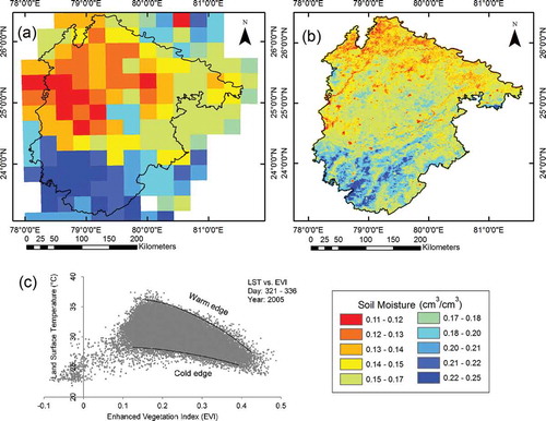
Figure 3. Spatial downscaling of soil moisture for composite 321–336, 2005. (a) Coarse spatial resolution soil moisture. (b) Spatially downscaled fine resolution soil moisture. (c) Triangular cloud formed from scatter plot between surface temperature and vegetation index. For full color versions of the figures in this paper, please see the online version.

3.1.4. Crop yield

Seasonal crop production at district level was downloaded from the website (https://data.gov.in/) available under the program “A Digital India Initiative.” This data provided acreage in hectares and production in tons for a specific crop in a specific agricultural season at a particular district which was used to calculate seasonal crop yield (Y_s) during the respective season. The districts of Madhya Pradesh were having data of Rabi season from 1999–2000 to 2008–2009 with a data gap in 2006–2007. On the other hand, districts of Uttar Pradesh were having continuous data from 1999–2000 to 2010–2011.

3.2. Preprocessing and framework

The entire methodology is presented as schematic flow process in Figure 2. Land surface temperature (LST) from MODIS and soil moisture from CCI, ESA were averaged to derive 16-day composites for matching with 16-day vegetation index product from MODIS. These 16-day composites were arranged according to respective years and Julian days to be called as temporal stage in a Rabi season (October–May). The Julian days 289th day of a year to 113th day of next year are covered in a Rabi agricultural season, making it as 13 temporal stages in a season. The key idea to utilize satellite soil moisture to detect agricultural drought at district scale was achieved through spatial downscaling by using enhanced vegetation index (EVI) and LST from MODIS. Before using SM_d, it was tested for statistical significance by comparing with SM_c. Also, SM_d was tested for having relationship as a dependent variable on 16-day EDI computed from daily rainfall; and the influencing variable for 16-day VCI derived from 16 daily MODIS NDVI. These reasonable evidences were used as to validate SM_d. It was followed by comparative performance of SM_d against VCI to detect decrease/increase in Y_s at district scale for major crop grown during seasons from 2003–2004 to 2008–2009. This detection process was applied at only Rabi agricultural areas which were identified from a unique method based on analysis of phonological behavior of MODIS NDVI. Finally, Rabi agricultural areas experiencing frequent occurrences of soil moisture deficiency from 2003–2004 to 2008–2009 were mapped to scale the spatial severity as a resultant of soil moisture deficiency. These areas were remarked as most concerned areas in Bundelkhand region from 2003 to 2009 for occurrence of Rabi agricultural drought.

3.3. Spatial downscaling of soil moisture

The blended soil moisture data from CCI, ESA is known to be showing several successful applications in drought related studies (Anderson et al. 2012; McNally et al. 2016; Rahmani, Golian, and Brocca 2016). However, it was unsuitable for thematic applications at district scale because of its coarse spatial resolution. It was downscaled to a finer spatial resolution by using vegetation index and surface temperature as demonstrated by Kim and Hogue (2012) and Zhao and Li (2013). Points cloud between warm and cold edge in triangle formed from the plot of vegetation index against surface temperature (Carlson, Gillies, and Perry 1994) was used to draw out statistical coefficients to be used in spatial downscaling of soil moisture. The triangle method has the potential to utilize large image data sets and turn out nonlinear solutions for availability (Carlson 2007). The preview of spatial downscaling of soil moisture for a sample composite image is shown in Figure 3. The vegetation index used for the downscaling was MODIS EVI with reduced soil background interference (Huete et al. 2002). It ensured that the predictions made for downscaled value of soil moisture remains purely within the dependency on corresponding vegetation and surface temperature. For each temporal stage, EVI and LST were spatially normalized within a range of 0–1 (Equation (1) and (2)). These variables were used as independent variables with SM_c being the dependent variable to get the coefficients of second-order polynomial regression (Equation (3)), which were used later for prediction of the downscaled soil moisture (Equation (4)):

(1)

(2)

(3)

(4)

EVI is enhanced vegetation index from MODIS, LST is land surface temperature from MODIS, the subscripts max and min represent the maximum and minimum parameter value over the spatial extent respectively, and subscript N represents normalized value with respect to spatial extent, SM_c is the coarse resolution soil moisture at a location, a_ij represents the set of coefficients from the second-order polynomial regression, and SM_d is the fine resolution soil moisture at the same location as that of SM_c.

The root-mean-square error (RMSE) between downscaled product and raw data for five sample areas as well as entire study area (Figure 4a) were calculated in order to validate the statistical significance of downscaled estimations around the spatial extent. The RMSE was computed as

(5)

Figure 4. (a) Rain gauge station and sample area distribution in the study area to test for statistical and physical significance. (b) RMSE between downscaled soil moisture and raw soil moisture in Bundelkhand region from Rabi seasons 2003–2004 to 2008–2009.

where RMSE is the root mean square error, i represents the sample area, x represents a pixel, n is the total number of pixels in a sample area, SM_c is raw soil moisture, and SM_d is the spatially downscaled soil moisture. The RMSE values for the study timespan (from 2003–2004 to 2008–2009) were found to be less than 0.065 cm³/cm³ (Figure 4b), which was considered reasonable to be used.

3.4. EDI

EDI is known to perform better than several popular indices in terms of number/feasibility of parameters required for derivation, time scale, simplicity and accuracy in assessment (Usman et al. 2005; Morid, Smakhtin, and Moghaddasi 2006). The present research was specific about spatial variability in agricultural drought due to which point-based temporal EDI was not used directly for monitoring agricultural drought. Instead, it was used to explain the aftereffects of rainfall/dry spells on soil moisture at rain gauge points, which validated the physical significance of SM_d. The properties reflected from the concept of effective precipitation in EDI was expected to be better for this work against some of the traditional meteorological drought indices like “Palmer drought severity index (PDSI)” (Palmer 1965) and “standardized precipitation index (SPI)” (McKee, Doesken, and Kleist 1995). EDI was calculated at eight rain gauge stations spread across the study area (Figure 4a) using daily rainfall data from January 1975 to December 2010 as shown in Byun and Wilhite (1999) and presented in Equations (6)–(8):

(6)

(7)

(8)

EP₃ is effective precipitation of a particular day accumulated for three days, P_m is the precipitation for a day m days prior to a specific day, DEP₃ is deviation of EP₃ from the mean of EP₃, that is, (MEP₃), and was calculated for each calendar date, in present case the mean value is estimated using daily data of 36 years (January 1975–December 2010), EDI₃ is the Effective drought index value and SD (DEP₃) is the standard deviation of DEP₃ in 36 years range. EDI calculated for daily scale was averaged to derive 16-daily EDI so as to match the time scale of SM_d.

3.5. VCI

NDVI from various optical sensors are the most widely used indicator to monitor vegetation health from remote sensing, but due to its normalized quantification in spatial dimension, it is irrelevant to be utilized directly for temporal monitoring. However, there are several derivatives of NDVI which are modified to provide magnitudes which could be used for the same. VCI is one of the popular derivatives of NDVI which has been used successfully in studies on temporal vegetation monitoring (Quiring and Ganesh 2010; Rhee, Im, and Carbone 2010). It is capable of targeting the change in NDVI at a point over a time period to quantify the vegetation condition irrespective of spatial geographical differences in vegetation types. VCI derived from NDVI for monitoring drought conditions have been studied in various regions around the world and have been shown to be strongly correlated with agricultural production in regions of South America, Africa, Asia, North America, and Europe, particularly during the critical periods of crop growth (Jiao et al. 2016). In the present study, VCI was derived from MODIS NDVI and was used as a competitor of SM_d to detect Y_s during Rabi seasons from 2003–2004 to 2008–2009. VCI was computed as

(9)

where for a spatial location, NDVI, NDVI_max, and NDVI_min are the observed, maximum, and minimum values, respectively, from historical NDVI in Rabi seasons over the time period and VCI is the derived vegetation condition index. The computed VCI in Rabi season was used for validating the physical significance of SM_d (Section 4.1.2) as well as a competitor of SM_d for efficiency in detecting trends in Y_s and monitoring seasonal agricultural drought (Section 4.2.1).

3.6. Identification of area under Rabi agriculture

MODIS product provides land cover at annual scale, which is improper for seasonal studies. There are several reasons for this unsuitability. First of all, it is less likely that a pixel classified as crop area will be entirely covered with agricultural area only. Second, it is also obvious that those pixels might not be in agricultural practice at all in Rabi season. Therefore, it is crucial to identify the pixels which were under Rabi agriculture. A unique method based on the crop phenology was used for distinction of cropped and non-cropped areas in the Rabi season.

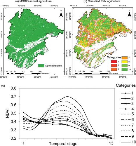
Since, MODIS land cover of a year represents the land classes as on the first day of that year, it was assumed to represent the Rabi season starting from the previous year. NDVI composites in Rabi season were ordered serially as temporal stages. The class “cropland” was selected from MCD12Q1 product for each year. It is evident that temporal plot of NDVI at a typical pixel with agricultural area will rise till the maturity of crops and descend toward harvesting phase (Figure 5). But pixels with less agricultural or drought affected zones will show the curve from corresponding temporal NDVI tending toward linear behavior with absolute linearity at no agriculture.

Figure 5. Temporal behavior of NDVI used in identifying Rabi crop.

This idea was utilized to separate the cropped and non-cropped pixels by using coefficient of determination (R²) of the linear fit for the plotted NDVI against temporal stage of the season at MODIS cropland class. Many times modeling of phonological behavior of crops had been related with higher degree polynomial curves. But it was inappropriate to use higher order regression as it has also the tendency to fit linear plots with good R² value, which would be inadequate for discrimination between temporal curves. While high R² value for linear fit indicates pixels with no agriculture (1 – R²) was used as a measure to identify pixels with probability of Rabi agriculture. The overall (1 – R²) images grouped into 10 categories (10% interval) were prepared from seasons 2003–2004 to 2009–2010 (Figure 6a and b) and the temporal curve of spatially averaged MODIS NDVI of the categories were used to recognize the phonological behavior of seasonal agriculture (Figure 6c). It was observed that NDVI for categories greater than or equivalent to fourth category exhibited behavior like agriculture due to which (1 – R²) for those pixels were considered as Rabi agricultural area. Temporal curves of spatially averaged NDVI strengthened the decision of using (1 – R²) for spotting pixels with Rabi crops. The identified categories were all together used as a united mask before any further estimation, so as to target the Rabi agriculture exclusively.

Figure 6. Identification of Rabi agriculture in Bundelkhand region for season 2004–2005. (a) MODIS annual agriculture in 2005. (b) Rabi agriculture in 2004–2005. (c) Temporal curves of spatially averaged NDVI in 2004–2005.

3.7. Soil moisture and vegetation condition as indicator of agricultural drought

Agricultural drought in terms of reduced Y_s could be detected by monitoring soil moisture and vegetation condition in the growth season. However, from temporal stages of a growth season, 13 quantities could not be used directly to match one value of Y_s for a season. It was necessary to derive a function, which represents the temporal quantities of soil moisture and vegetation health. Hence, time of soil moisture deficiency and time of vegetation condition below normal during a Rabi season were calculated. Time function of these parameters was chosen as the indicator because agricultural drought is believed to result from prolonged period of stress (Narasimhan and Srinivasan 2005). In this work, the time of stress that could be reflected from SM_d and VCI at district scale is estimated as shown in Equations (10)–(13):

(10)

(11)

(12)

(13)

Here, s represents a Rabi season, i represents temporal stage, ⁱSM_s is the SM_d in a temporal stage of a season, n_s is the number of seasons, ⁱSM_m is the mean of soil moisture in for a particular temporal stage in overall the seasons, ⁱSM_def,_s is the soil moisture deficiency experienced in a temporal stage of a season, ⁱD_s represents 1 or 0 based on a soil moisture deficiency or excess in a season, respectively, n_i is the number of temporal stages in a season and FSM_s represents the ratio of time in which soil moisture deficiency is experienced to time duration in Rabi season. Time function from VCI (FVCI_s) was also calculated in the same fashion as FSM_s derived from SM_d. These functions were used as indicators of agricultural drought. A common period of Rabi seasons from 2003–2004 to 2008–2009 was focused due to availability of all data, especially SM_d.

The time function computed from SM_d and VCI were compared in terms of performance to detect agricultural drought. Trend followed by the computed time functions, FSM_s and FVCI_s were plotted with Y_s at district scale. However, these functions were inappropriate to be used directly because of scale differences with Y_s. Also, these functions hold inverse relation with Y_s as with higher FSM_s and FVCI_s values, the vegetation is supposed to tend more toward agricultural drought resulting in reduced yield. In simpler words, high value of these functions indicates low value of Y_s. Therefore, complementary values of the normalized time function, FSM_s and FVCI_s were plotted against normalized Y_s to resolve the issues of scale and inverse relation (Equations (14)–(16)):

(14)

(15)

(16)

Here, for the Rabi seasons (s varying from 2003–2004 to 2008–2009), SM deficit and VCI deficit are the derivatives from FSM_s and FVCI_s, respectively, N_yield is normalized Y_s of major crop practiced in a district. SM deficit signify time of dry spell whereas, VCI deficit signify time of poor vegetation condition; eventually both of these derivatives signify stressed condition of crops.

4. Results and discussions

This section discusses the validity of SM_d to be used for identification and monitoring of Rabi agricultural drought. However, limitations due to unavailability of in-situ soil moisture during the study period made it challenging for any direct validation. Therefore, the best possible way out was to check the temporal dependency of soil moisture on rainfall/dry spells and spatiotemporal dependency of vegetation on soil moisture, which validates by agreeing with natural processes in a way. This section also discusses the identification of Rabi agricultural drought at district scale and hence, spatiotemporal detection and monitoring of seasonal agricultural drought.

4.1. Validation of downscaled soil moisture

It is important that the SM_d should show relationship with other variables of natural process at both temporal and spatial domains which validates its use in agricultural drought detection and monitoring. To be precise, post effects of EDI on SM_d and post effects of SM_d on VCI is discussed through linear correlation coefficient (R).

4.1.1. Effect of rainfall and dry spells on soil moisture

Direct analysis of soil moisture after a rainfall event to trace the effects might not be useful if the antecedent condition is already wet. Hence, EDI was used, which is based on the concept of effective precipitation to show the persisting effects of rainfall or dry spell. Sixteen-daily EDI were used to match the scale of 16-day soil moisture. Figure 7 discusses the comparison between temporal plots of EDI against SM_c and EDI against SM_d at the rain gauge stations. The values of SM_c and SM_d were taken from the respective pixels on which the rain gauge stations are installed. High EDI values (EDI >1.5) were removed as outlier, which represented wet condition. It was observed that EDI derived from rainfall have a positive correlation in both plots which indicates that rainfall have immediate effects on soil moisture. It was also noticed that SM_d have higher correlation with EDI in comparison to SM_c at all instances. SM_d was found to be influenced by persisting effects of rainfall or dry spell events. However, the range of R between SM_d as dependent and EDI as independent variable varied from 0.5 to 0.7. This moderate range of correlation coefficient could be due to pre-existing irrigation water. Still, the presence of positive R values justifies the validity of the downscaled derivative as it approved EDI as an influencing parameter on SM_d.

Figure 7. Scatter plots between EDI and soil moisture at rain gauge stations.

4.1.2. Effect of soil moisture on vegetation

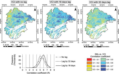
In general, the influence of soil moisture on vegetation could be seen effective within the parallel timespan or later. To expose the same, SM_d was temporally correlated with VCI in the parallel timespan, lagging by 16 days, and lagging by 32 days for the Rabi seasons in agricultural areas obtained from MODIS annual land cover. Figure 8 shows spatial distribution of temporal R values for SM_d against VCI mapped in agricultural areas of Bundelkhand region in Rabi seasons (2003–2004 to 2008–2009). Large distribution of positive R values was observed around the study area which shows the spatiotemporal dependency of vegetation on soil moisture. Negative correlation values are omitted owing to negligible distribution. Histogram analysis at the comparative level showed that VCI lagging by 16 days to SM_d exhibits increasing R in both frequency and quantity than VCI with no lag to SM_d and VCI with a lag of 32 days. It shows high frequency in second image with a narrow curve for a range of R value with lower and higher limits in comparison to first and third images. R value in several areas in the first image from left could be seen increasing in second image. Also, R value in most of areas in second image further reduces in third image in spatial extent. Therefore, conclusion was drawn, that vegetation condition lagging by 16 days is most affected by soil moisture than that of parallel time and after 32 days. With the presence of positive R values, it was validated that vegetation is influenced by soil moisture represented by SM_d. Hence, the spatiotemporal dependency of VCI on SM_d was found which validated the downscaled product.

Figure 8. Spatial correlation coefficient (R) of SM_d against VCI in Rabi seasons 2003–2004 to 2008–2009 in MODIS agricultural areas.

4.2. Identification of Rabi agricultural drought

The term “agricultural drought” could be confusing with low production of crops which could result from two major reasons. They are due to low agricultural acreage and low yield in a growth season. The former was not focused as agricultural drought is truly denoted by reduced Y_s.

4.2.1. Soil moisture and VCI deficits

The derivatives (SM deficit and VCI deficit) from Equation (14) and (15) were used to detect rise/fall in N_yield, which is normalized Y_s (Equation (16)) for major crop practiced in a district (Figure 9a–m). The trend of SM deficit and VCI deficit were observed to capture well the fluctuations in N_yield. Comparison between performances of SM deficit against VCI deficit to detect N_yield carried out at district level is shown in Figure 9(a–m). In case of SM deficits against N_yield, highest R was found as 0.93 for Jhansi with simultaneous R for VCI deficit as 0.86 (Table 1). The lowest R for SM deficit was 0.59 for Tikamgarh with simultaneous R for VCI deficits as 0.71. The reverse analogy showed highest and lowest R for VCI deficits in Chattarpur and Damoh as 0.94 and 0.33 with simultaneous R for SM deficit as 0.86 and 0.85. On a scale of 13 districts, 11 showed better association of N_yield with SM deficit than VCI deficit. Also, the highest N_yield at 11 districts were successfully detected by FSM_s in comparison to four times by FVCI_s. SM deficit outperformed VCI deficit to detect the least N_yield absolutely at all instances which are represented as the worst agricultural drought season.

Table 1. Comparative analysis for association of SM deficit and VCI deficit with normalized crop yield of the major crop in the districts in Rabi seasons (2003–2004 to 2008–2009) in Bundelkhand region.

District	Correlation coefficient against Nyield		NSE coefficient against Nyield
	SM deficits	VCI deficits	SM deficits	VCI deficits
Banda	0.86	0.71	0.64	0.37
Chattarpur	0.87	0.94	0.68	0.86
Chitrakoot	0.91	0.58	0.52	−0.29
Damoh	0.85	0.33	0.56	−0.70
Datia	0.62	0.54	−0.15	−0.10
Hamirpur	0.82	0.60	0.51	−0.12
Jalaun	0.80	0.73	0.26	0.13
Jhansi	0.93	0.86	0.77	0.71
Lalitpur	0.92	0.65	0.82	0.01
Mahoba	0.90	0.72	0.71	0.14
Panna	0.66	0.50	−0.03	−1.04
Sagar	0.91	0.68	0.63	0.04
Tikamgarh	0.59	0.71	−0.19	−0.19

Figure 9. Identification of Rabi agricultural drought from 2003–2004 to 2008–2009 using SM deficits and VCI deficits at district scale for (a) Banda, (b) Chattarpur, (c) Chitrakoot, (d) Damoh, (e) Datia, (f) Hamirpur, (g) Jalaun, (h) Jhansi, (i) Lalitpur, (j) Mahoba, (k) Panna, (l) Sagar, (m) Tikamgarh.

Figure 9. (Continued)

Nash–Sutcliffe efficiency (NSE) coefficient was also computed for SM deficit and VCI deficit against N_yield considered as observed parameter. NSE was computed as shown in Equation (17):

(17)

where for the Rabi seasons (s varying from 2003–2004 to 2008–2009), N_yield is the respective normalized Y_s, Xdeficit is the parameter to be used as respective seasonal SM deficit and VCI deficit, and is the mean of all seasonal N_yield of a district and NSE is the NSE coefficient. The computed NSE for all the districts are presented in Table 1 where it could be understood that SM deficit have better value within the range between 0 and 1 at most of the occasions than VCI deficit. It shows that SM deficit has more capability to explain the trends in seasonal variation in N_yield. Overall observations suggested FSM_s to be the better indicator as compared to FVCI_s for spatiotemporal agricultural drought detection and monitoring in Rabi seasons. The R values and NSE values at the district scale indicated stronger association of seasonal crop yield with soil moisture than that with vegetation condition derived from MODIS. Agricultural drought occurrence was found to be well captured with high FSM_s around the study area and soil moisture was proved to be a powerful indicator in present research.

4.2.2. Spatiotemporal Rabi agricultural drought

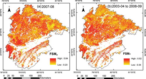
Efficiency of soil moisture to detect seasonal agricultural drought was promising and hence FSM_s from SM_d was used for mapping the agricultural drought affected areas in Bundelkhand region due to frequent soil moisture deficiency during Rabi seasons. Figure 10a shows FSM_s for season 2007–2008, which was the worst agricultural drought period interpreted from Y_s. It was observed that during this period, deficiency in soil moisture was faced from 23% to 84% of times in the growth period in the Rabi agricultural areas. Here, FSM_s shows the spatial severity of soil moisture deficit tending crops toward reduction in yield in 2007–2008. The function FSM_s was also applied to map for overall seasons (2003–2004 to 2008–2009) which is presented in Figure 10b. It was understood that Rabi agricultural areas of Bundelkhand region faced soil moisture deficiency from 34% to 52% of times in 6 years. It presents the spatial severity in the region where high FSM_s represents the most concerned areas toward agricultural drought due to frequent soil moisture deficiency in 2003–2004 to 2008–2009. The maps show spatiotemporal traces of seasonal agricultural drought captured by soil moisture.

Figure 10. Spatial distribution of time function of soil moisture deficiency, FSMs for the Rabi seasons in Bundelkhand region. (a) Season 2007–2008. (b) Seasons 2003–2004 to 2008–2009.

5. Conclusion

The present study demonstrates the use of blended soil moisture product from various passive and active microwave sensors for detecting the agricultural drought in Rabi season in Bundelkhand region of India. This soil moisture product at coarse spatial resolution was obtained from European space agency (ESA) under the CCI program. The present research aimed to utilize a novel time-based function of soil moisture (FSM_s) as an effective indicator to identify departure in seasonal crop yield (Y_s) in temporal dimension and use it to monitor in spatial dimension at district scale. The objective of functioning at district scale was accomplished by spatial downscaling coarse resolution soil moisture (SM_c) to fine resolution soil moisture (SM_d) by using triangle method incorporating EVI and LST from MODIS. The RMSE between SM_c and SM_d tested for randomly selected sample areas as well as entire study area showed to be under 0.065 cm³/cm³. SM_d was seen to be showing dependency on EDI derived from point meteorological sources and influencing VCI derived from MODIS NDVI. It agreed with the natural phenomenon of soil moisture depending on rainfall events/dry spells and vegetation condition depending on soil moisture, which validated the downscaling of SM_d. A unique method was used to identify agricultural areas in Rabi season by using the phonological behavior of MODIS NDVI and it was used as mask for any further estimation. Time functions of soil moisture (FSM_s) and MODIS vegetation condition index (FVCI_s) representing frequent dry spells and duration of poor vegetation condition respectively, showed capability to capture the trend in Y_s at district scale. However, for all districts the Rabi season of year 2007–2008 (least Y_s or worst agricultural drought season) was detected by FSM_s better than FVCI_s, that is, at 10 out of 13 districts with correlation coefficient (R ≥0.8). Also, the highest seasonal crop yields at 11 districts were successfully detected using FSM_s as compared to four times by using FVCI_s. At the same scale, NSE coefficient was found to be better for FSM_s than FVCI_s at 10 occasions. Comparison revealed that on a regional scale, the efficiency to capture trends in Y_s is better by using SM_d than VCI. The reason could be inferred as stronger association of crop yield with soil moisture than that with vegetation condition during an agricultural season. Soil moisture form satellite source such as SMMR on board Nimbus 7, SSM/I on board DMSP satellites, TMI on board TRMM satellites and AMSR-E on board Aqua platform is concluded as a powerful spatiotemporal indicator for seasonal agricultural drought detection and monitoring at spatial scale of district level. Furthermore, the areas of Rabi agricultural drought severity were mapped for the worst Rabi season as well as overall seasons using FSM_s as a result drawn from the strong relationship between seasonal crop yield and duration of soil moisture scarcity.

However, cloud cover creates some limitations for the methodology as spatial downscaling of the soil moisture could not be carried out due to unavailability of optical and thermal data. This problem was dealt with the use of 16-day MODIS EVI and LST composites, which increased the chances of spatial visibility in the downscaled product. The present work was not affected from cloud cover as Rabi season experiences scanty cloud cover in this region. But, the method has its limitations in terms of seasonality where monsoonal conditions could not be overcome. The scope of this study could be enhanced in future studies by using land cover according to different crop type and operational spaceborne soil moisture data from sources such as SMOS, SMAP, etc. It can be useful for spatiotemporal seasonal agricultural drought assessment and monitoring at high spatial resolution which can cover up to sub-regional scale in arid and semi-arid regions.

Acknowledgments

Authors’ sincere appreciation is extended to HoD, Department of Civil Engineering, IIT Guwahati, for providing computational facilities to carry out this work. We are also obligated to ESA for providing free access to satellite soil moisture product under CCI program and NASA for MODIS products. Authors also acknowledge the editor and anonymous reviewers for their inputs.

Disclosure statement

No potential conflict of interest was reported by the authors.

References

- Aggarwal, P. K. 2008. “Global Climate Change and Indian Agriculture: Impacts, Adaptation and Mitigation.” The Indian Journal of Agricultural Sciences 78 (11): 911-919.
- Anderson, W. B., B. F. Zaitchik, C. R. Hain, M. C. Anderson, M. T. Yilmaz, J. Mecikalski, and L. Schultz. 2012. “Towards an Integrated Soil Moisture Drought Monitor for East Africa.” Hydrology and Earth System Sciences 16: 2893–2913. doi:10.5194/hess-16-2893-2012.
- Boken, V. K., A. P. Cracknell, and R. L. Heathcote. 2005. Monitoring and Predicting Agricultural Drought: A Global Study. New York: Oxford University Press.
- Bolten, J. D., W. T. Crow, X. Zhan, T. J. Jackson, and C. A. Reynolds. 2010. “Evaluating the Utility of Remotely Sensed Soil Moisture Retrievals for Operational Agricultural Drought Monitoring.” IEEE Journal of Selected Topics in Applied Earth Observations and Remote Sensing 3 (1): 57–66. doi:10.1109/JSTARS.2009.2037163.
- Byun, H.-R., and D. A. Wilhite. 1999. “Objective Quantification of Drought Severity and Duration.” Journal of Climate 12 (9): 2747–2756. doi:10.1175/1520-0442(1999)012<2747:OQODSA>2.0.CO;2.
- Carlson, T. N., R. R. Gillies, and E. M. Perry. 1994. “A Method to Make Use of Thermal Infrared Temperature and NDVI Measurements to Infer Surface Soil Water Content and Fractional Vegetation Cover.” Remote Sensing Reviews 9 (1–2): 161–173. doi:10.1080/02757259409532220.
- Carlson, T. 2007. “An Overview of the “Triangle Method” for Estimating Surface Evapotranspiration and Soil Moisture from Satellite Imagery.” Sensors 7 (8): 1612–1629. doi:10.3390/s7081612.
- Du, Y., F. T. Ulaby, and M. C. Dobson. 2000. “Sensitivity to Soil Moisture by Active and Passive Microwave Sensors.” IEEE Transactions on Geoscience and Remote Sensing 38 (1): 105–114. doi:10.1109/36.823905.
- Farooq, M., A. Wahid, N. Kobayashi, D. Fujita, and S. M. A. Basra. 2009. “Plant Drought Stress: Effects, Mechanisms and Management.” Agronomy for Sustainable Development 29 (1): 185–212. doi:10.1051/agro:2008021.
- Gago, J., C. Douthe, R. E. Coopman, P. P. Gallego, M. Ribas-Carbo, J. Flexas, J. Escalona, and H. Medrano. 2015. “Uavs Challenge to Assess Water Stress for Sustainable Agriculture.” Agricultural Water Management 153: 9–19. doi:10.1016/j.agwat.2015.01.020.
- Guha, A., and V. Lakshmi. 2004. “Use of the Scanning Multichannel Microwave Radiometer (SMMR) to Retrieve Soil Moisture and Surface Temperature over the Central United States.” IEEE Transactions on Geoscience and Remote Sensing 42 (7): 1482–1494. doi:10.1109/TGRS.2004.828193.
- Holzman, M. E., R. Rivas, and M. C. Piccolo. 2014. “Estimating Soil Moisture and the Relationship with Crop Yield Using Surface Temperature and Vegetation Index.” International Journal of Applied Earth Observation and Geoinformation 28 (1): 181–192. doi:10.1016/j.jag.2013.12.006.
- Huete, A., K. Didan, T. Miura, E. P. Rodriguez, X. Gao, and L. G. Ferreira. 2002. “Overview of the Radiometric and Biophysical Performance of the MODIS Vegetation Indices.” Remote Sensing of Environment 83 (1–2): 195–213. doi:10.1016/S0034-4257(02)00096-2.
- Jiao, W., L. Zhang, Q. Chang, D. Fu, Y. Cen, and Q. Tong. 2016. “Evaluating an Enhanced Vegetation Condition Index (VCI) Based on VIUPD for Drought Monitoring in the Continental United States.” Remote Sensing 8 (3): 224. doi:10.3390/rs8030224.
- Kim, J., and T. S. Hogue. 2012. “Improving Spatial Soil Moisture Representation through Integration of AMSR-E and MODIS Products.” IEEE Transactions on Geoscience and Remote Sensing 50 (2): 446–460. doi:10.1109/TGRS.2011.2161318.
- Kogan, F. N. 1990. “Remote Sensing of Weather Impacts on Vegetation in Non-Homogeneous Areas.” International Journal of Remote Sensing 11 (8): 1405–1419. doi:10.1080/01431169008955102.
- Kondratyev, K. Y., V. V. Melentyev, Y. I. Rabinovich, and E. M. Shulgina. 1977. “Passive Microwave Remote Sensing of Soil Moisture.” Proceedings of 11th International Symposium on Remote Sensing Environment, April 25-29, 1977, University of Michigan, Ann Arbor, USA, 1641-1661.
- Liu, Y. Y., W. A. Dorigo, R. M. Parinussa, R. A. M. De Jeu, W. Wagner, M. F. McCabe, J. P. Evans, and A. I. J. M. Van Dijk. 2012. “Trend-Preserving Blending of Passive and Active Microwave Soil Moisture Retrievals.” Remote Sensing of Environment 123: 280–297. doi:10.1016/j.rse.2012.03.014.
- Liu, Y. Y., R. M. Parinussa, W. A. Dorigo, R. A. M. De Jeu, W. Wagner, A. I. J. M. Van Dijk, M. F. McCabe, and J. P. Evans. 2011. “Developing an Improved Soil Moisture Dataset by Blending Passive and Active Microwave Satellite-Based Retrievals.” Hydrology and Earth System Sciences 15 (2): 425–436. doi:10.5194/hess-15-425-2011.
- Mao, Y., Z. Wu, H. He, G. Lu, H. Xu, and Q. Lin. 2017. “Spatio-Temporal Analysis of Drought in a Typical Plain Region Based on the Soil Moisture Anomaly Percentage Index.” Science of the Total Environment 576: 752–765. doi:10.1016/j.scitotenv.2016.10.116.
- McKee, T. B., N. J. Doesken, and J. Kleist. 1995. “Drought Monitoring with Multiple Time Scales.”Proceedings of the 9th American Meteorological Society Conference on Applied Climatology, January 15-20, 1995, Dallas, TX, USA, 233–236. http://ccc.atmos.colostate.edu/droughtmonitoring.pdf
- McNally, A., S. Shukla, K. R. Arsenault, S. Wang, C. D. Peters-Lidard, and J. P. Verdin. 2016. “Evaluating ESA CCI Soil Moisture in East Africa.” International Journal of Applied Earth Observation and Geoinformation 48: 96–109. doi:10.1016/j.jag.2016.01.001.
- Mishra, A. K., and V. P. Singh. 2010. “A Review of Drought Concepts.” Journal of Hydrology 391 (1–2): 202–216. doi:10.1016/j.jhydrol.2010.07.012.
- Morid, S., V. Smakhtin, and M. Moghaddasi. 2006. “Comparison of Seven Meteorological Indices for Drought Monitoring in Iran.” International Journal of Climatology 26 (7): 971–985. doi:10.1002/joc.1264.
- Narasimhan, B., and R. Srinivasan. 2005. “Development and Evaluation of Soil Moisture Deficit Index (SMDI) and Evapotranspiration Deficit Index (ETDI) for Agricultural Drought Monitoring.” Agricultural and Forest Meteorology 133: 69–88. doi:10.1016/j.agrformet.2005.07.012.
- National Rainfed Area Authority. 2008. Report on Drought Mitigation Strategy for Bundelkhand Region of Uttar Pradesh and Madhya Pradesh.
- Njoku, E. G., and D. Entekhabi. 1996. “Soil Moisture Theories and Observationspassive Microwave Remote Sensing of Soil Moisture.” Journal of Hydrology 184 (1–2): 101–129. doi:10.1016/0022-1694(95)02970-2.
- Palmer, W. C. 1965. “Meteorological Drought.” U.S. Weather Bureau Research Paper 45:58.
- Patel, N. R., and K. Yadav. 2015. “Monitoring Spatio-Temporal Pattern of Drought Stress Using Integrated Drought Index over Bundelkhand Region, India.” Natural Hazards 77 (2): 663–677. doi:10.1007/s11069-015-1614-0.
- Pérez-Blanco, C. D., G. Standardi, J. Mysiak, R. Parrado, and C. Gutiérrez-Martín. 2016. “Incremental Water Charging in Agriculture. A Case Study of the Regione Emilia Romagna in Italy.” Environmental Modelling & Software 78: 202–215. doi:10.1016/j.envsoft.2015.12.016.
- Quiring, S. M., and S. Ganesh. 2010. “Evaluating the Utility of the Vegetation Condition Index (VCI) for Monitoring Meteorological Drought in Texas.” Agricultural and Forest Meteorology 150: 330–339. doi:10.1016/j.agrformet.2009.11.015.
- Rahmani, A., S. Golian, and L. Brocca. 2016. “Multiyear Monitoring of Soil Moisture over Iran through Satellite and Reanalysis Soil Moisture Products.” International Journal of Applied Earth Observation and Geoinformation 48: 85–95. doi:10.1016/j.jag.2015.06.009.
- Reichle, R. H., R. D. Koster, J. Dong, and A. A. Berg. 2004. “Global Soil Moisture from Satellite Observations, Land Surface Models, and Ground Data: Implications for Data Assimilation.” Journal of Hydrometeorology 5 (3): 430–442. doi:10.1175/1525-7541(2004)005<0430:GSMFSO>2.0.CO;2.
- Rhee, J., J. Im, and G. J. Carbone. 2010. “Monitoring Agricultural Drought for Arid and Humid Regions Using Multi-Sensor Remote Sensing Data.” Remote Sensing of Environment 114 (12): 2875–2887. doi:10.1016/j.rse.2010.07.005.
- Rockström, J., J. Barron, and P. Fox. 2002. “Rainwater Management for Increased Productivity among Small-Holder Farmers in Drought Prone Environments.” Physics and Chemistry of the Earth, Parts A/B/C 27 (11–22): 949–959. doi:10.1016/S1474-7065(02)00098-0.
- Rockström, J., and M. Falkenmark. 2000. “Semiarid Crop Production from a Hydrological Perspective: Gap between Potential and Actual Yields.” Critical Reviews in Plant Sciences 19 (4): 319–346. doi:10.1080/07352680091139259.
- Senay, G. B., N. M. Velpuri, S. Bohms, M. Budde, C. Young, J. Rowland, and J. P. Verdin. 2015. “Chapter 9. “Drought Monitoring and Assessment: Remote Sensing and Modeling Approaches for the Famine Early Warning Systems Network”. In Hydro-Meteorological Hazards, Risks and Disasters, edited by J. F. Shroder, P. Paron, and G. Di Baldassarre, 233–262. Boston, MA: Elsevier. doi:10.1016/B978-0-12-394846-5.00009-6.
- Seshasai, M. V. R., C. S. Murthy, K. Chandrasekar, A. T. Jeyaseelan, P. G. Diwakar, and V. K. Dadhwal. 2016. “Agricultural Drought: Assessment & Monitoring.” Mausam 67 (1): 131–142. http://metnet.imd.gov.in/mausamdocs/167111.pdf.
- Shinde, S. S., and P. Modak. 2013. “Chapter 2.14. “Vulnerability of Indian Agriculture to Climate Change.”.” In Climate Vulnerability, edited by R. A. Pielke, 139–152. Oxford: Academic Press. doi:10.1016/B978-0-12-384703-4.00227-6.
- Singh, R. P., S. Roy, and F. Kogan. 2003. “Vegetation and Temperature Condition Indices from NOAA AVHRR Data for Drought Monitoring over India.” International Journal of Remote Sensing 24 (22): 4393–4402. doi:10.1080/0143116031000084323.
- Thenkabail, P. S., M. S. D. N. Gamage, and V. U. Smakhtin. 2004. “The Use of Remote Sensing Data for Drought Assessment and Monitoring in Southwest Asia.” Research Report 85. Colombo, Sri Lanka: International Water Management Institute.
- Usman, M. T., E. Archer, P. Johnston, and M. Tadross. 2005. “A Conceptual Framework for Enhancing the Utility of Rainfall Hazard Forecasts for Agriculture in Marginal Environments.” Natural Hazards 34 (1): 111–129. doi:10.1007/s11069-004-4349-x.
- Wagner, W., W. Dorigo, R. De Jeu, D. Fernandez, J. Benveniste, E. Haas, and M. Ertl. 2012. “Fusion of Active and Passive Microwave Observations to Create an Essential Climate Variable Data Record on Soil Moisture.” ISPRS Annals of the Photogrammetry, Remote Sensing and Spatial Information Sciences I–7: 315–321. doi:10.5194/isprsannals-I-7-315-2012.
- Wilhite, D. A. 2000. “Chapter 1.” In Drought: A Global Assessment, edited by D. A. Wilhite, 3–18. London: Routledge.
- Wilhite, D. A. 2005. Drought and Water Crises: Science, Technology, and Management Issues. Vol. 86. Boca Raton, FL: CRC Press, Taylor & Francis Group.
- Wu, D., J. J. Qu, and X. Hao. 2015. “Agricultural Drought Monitoring Using MODIS-Based Drought Indices over the USA Corn Belt.” International Journal Of Remote Sensing 36 (21): 5403–5425. doi:10.1080/01431161.2015.1093190.
- Zhang, L., W. Jiao, H. Zhang, C. Huang, and Q. Tong. 2017. “Studying Drought Phenomena in the Continental United States in 2011 and 2012 Using Various Drought Indices.” Remote Sensing of Environment 190: 96–106. doi:10.1016/j.rse.2016.12.010.
- Zhao, W., and A. Li. 2013. “A Downscaling Method for Improving the Spatial Resolution of AMSR-E Derived Soil Moisture Product Based on MSG-SEVIRI Data.” Remote Sensing 5 (12): 6790–6811. doi:10.3390/rs5126790.