Creating high-resolution bare-earth digital elevation models (DEMs) from stereo imagery in an area of densely vegetated deciduous forest using combinations of procedures designed for lidar point cloud filtering

Abstract

For areas of the world that do not have access to lidar, fine-scale digital elevation models (DEMs) can be photogrammetrically created using globally available high-spatial resolution stereo satellite imagery. The resultant DEM is best termed a digital surface model (DSM) because it includes heights of surface features. In densely vegetated conditions, this inclusion can limit its usefulness in applications requiring a bare-earth DEM. This study explores the use of techniques designed for filtering lidar point clouds to mitigate the elevation artifacts caused by above ground features, within the context of a case study of Prince William Forest Park, Virginia, USA. The influences of land cover and leaf-on vs. leaf-off conditions are investigated, and the accuracy of the raw photogrammetric DSM extracted from leaf-on imagery was between that of a lidar bare-earth DEM and the Shuttle Radar Topography Mission DEM. Although the filtered leaf-on photogrammetric DEM retains some artifacts of the vegetation canopy and may not be useful for some applications, filtering procedures significantly improved the accuracy of the modeled terrain. The accuracy of the DSM extracted in leaf-off conditions was comparable in most areas to the lidar bare-earth DEM and filtering procedures resulted in accuracy comparable of that to the lidar DEM.

Keywords:

• Digital elevation model (DEM)
• Digital surface model (DSM)
• high-spatial resolution photogrammetric DSM
• filtering
• vegetation artifact

Introduction

Digital elevation models (DEMs) provide three-dimensional (3D) information that can be vital for effective geospatial analysis (Maune 2007; Tarolli 2014; DeWitt, Warner, and Conley 2015; Chirico, Malpeli, and Trimble 2012; Maxwell and Warner 2015; Maxwell, Warner, and Strager 2016). However, fine-scale, publically available DEMs have been generated for only limited areas of the world, placing a major constraint on the potential use of elevation information in remote-sensing analysis. Light detection and ranging (lidar) sensors, which use precise distance calculation of laser pulse return time to calculate the elevation of a surface, have become the principle means of collecting accurate and precise elevation data. The wavelengths and sensors utilized by such systems allow for the detection of multiple returns from semipermeable layers of the reflective surface, such as vegetation overlying the ground surface. More importantly, the density of point data collected by the lidar system may substantially impact the consistency of ground detection, particularly in dense forest vegetation (Chu et al. 2014). The dataset collected by lidar sensors is typically represented by an unstructured point cloud of elevations, which together quantify the ground surface and any overlying features. Classification of this point cloud into ground returns and above ground features is performed by a variety of methods, selected by the specific characteristics of the area of interest (Meng, Currit, and Zhao 2010; Sithole and Vosselman 2004; Mongus and Borut 2012; Axelsson 1999; Kraus and Pfeifer 1998; Montealegre, Lamelas, and De Riva. 2015). Although lidar is ideal for comprehensive quantification of ground and above ground feature elevations, contracting lidar data for new areas can be expensive and logistically impractical in remote areas of the world lacking air transportation infrastructure.

Fine-scale elevation data can also be generated from globally available high-spatial resolution satellite stereoscopic imagery, at substantially less cost than lidar acquisition, using computerized photogrammetric methods. These methods calculate the z (or elevation) dimension through measurement of parallax displacement in overlapping images (Wolf, Dewitt, and Wilkinson 2014; Haala et al. 2010). Recent advances in this field have automated the image-matching algorithms (Wohlfeil et al. 2012) that transform the mathematical relationship between two-dimensional image space to 3D object space (Ni et al. 2014; Toutin 2004). These matched-pixel locations produce a series of x, y, z measurements from which a DEM can be interpolated (Ni et al. 2014; Leberl et al. 2010; Toutin 2004). The resultant raster is best termed a digital surface model (DSM), wherein z-values indicate the elevation of the bare-earth ground surface plus the height of any above ground features (also referred to as the “reflective surface”). This is in contrast to a DEM, which refers to a raster with z-values indicating the elevation of the bare-earth surface, which could be used for hydrologic modeling (Maune 2007). Photogrammetry and other methods of 3D image matching have been found to produce highly accurate DSMs in bare areas (Sefercik et al. 2013; Müller et al. 2014; Bühler, Marty, and Ginzler 2012), however the presence vegetation or man-made features complicates the extraction of a bare-earth terrain model (Ressl et al. 2016; Müller et al. 2014). Removal of these above ground features from the DSM is necessary for any geospatial application requiring a bare-earth DEM. Thus, analysts considering the use of high-spatial resolution satellite imagery for generating their own DEMs are faced with multiple questions regarding how to reduce or remove the elevations that represent above ground features. Additionally, for deciduous forests, the optimal season for image acquisition is not obvious. Leaf-on vegetation may obscure the ground surface, but leaf-off imagery may provide complex shadowing and branch patterns that may not necessarily be good for producing bare-earth DEMs.

This study explores the use of commercially available processing techniques designed for lidar point cloud data to filter vegetation and other above ground features from a photogrammetrically derived DSM in forested environments with little or no built structures. Lidar-derived and photogrammetrically derived point clouds are compared to explore the potential of such tools in classifying and filtering elevation points belonging to vegetation from the DSM in an area of dense deciduous forest canopy. Then various combinations of lidar processing techniques are evaluated to determine their effectiveness in mitigating the above ground elevations of the DSM. In order to assess the utility of such techniques in areas of dense vegetation canopy, both leaf-on and leaf-off photogrammetrically created DSMs are examined. Additional processing techniques utilizing only ancillary data gathered from the source imagery or photogrammetric DSM are explored, and the influence of land cover and vegetation canopy height on vertical accuracy of filtered DEMs are evaluated.

Study area

An area of Prince William Forest Park (PWFP), in Northern Virginia, USA, was selected (Figure 1) for its location and data availability. Land cover within this area is predominantly mature forest, with some small open or grassy areas, and few buildings. Forest vegetation within the greater region is characterized as “eastern deciduous forest,” with 33 different tree species, all but 4 of which are deciduous. Predominant species include tulip poplar (Liriodendron tulipifera), Virginia pine (Pinus virginiana), American beech (Fagus gradiofolia), red maple (Acer rubrum), and white oak (Quercus alba) (Schmit, Campbell, and Parrish 2010, National Park Service 2016). Both tree age and forest structure vary spatially, with canopy height averaging 24.7 m and ranging from 0 to 45 m (Nortrup and Lehman 2013).

Figure 1. Study area within Prince William Forest Park in Prince William County, Virginia, USA. Mapped on Worldview-3 visible bands 5-red, 3-green, 2-blue, collected on October 6, 2014.

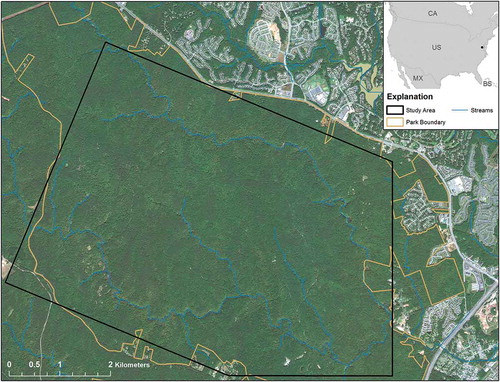
The dense, closed-canopy deciduous and evergreen forestland cover of the region, coupled with its moderate topography was chosen to exemplify the strengths and weaknesses of photogrammetrically derived high-resolution DEMs and the filtering techniques explored in this study because they create an ideally challenging scenario for mapping ground elevations. The methods investigated here are evaluated in the context of predominantly forested areas, and the results may not be directly applicable to urban areas with large buildings.

Data

Data used in this study (Table 1) include several types of satellite and aerial imagery, as well as multiple digital elevation datasets. High-resolution satellite imagery acquired from DigitalGlobe includes stereoscopic panchromatic 0.5 m GSD WorldView-1 imagery, monoscopic 4 band multispectral 1.5 m GSD WorldView-3 (Figure 1) imagery, and stereoscopic panchromatic 0.5 m GSD WorldView-3 imagery. The stereoscopic WorldView-1 was collected on 10 October 2015 and the monoscopic WorldView-3 imagery was collected on 6 October 2015, during the leaf-on phase of vegetation canopy in the study area. The stereoscopic WorldView-3 imagery, collected on 7 March 2016 captures the leaf-off phase of vegetation canopy. Aerial high-resolution orthoimagery collected during the spring of 2013 was used for accuracy assessment of the land cover classification (details of which can be found in Appendix A).

Table 1. Data used in the study.

	Satellite/source	Date (season)	View type	Characteristics	Pixel size (m)	Used for
Digital imagery
	WorldView-1	10 October 2015 (Leaf on)	Stereo	Panchromatic	0.5	Photogrammetric DSM
	WorldView-3	6 October 2015 (Leaf on)	Mono	Multispectral 4 band (VIS-NIR)	1.5	Classification of land cover
	WorldView-3	7 March 2016 (Leaf off)	Stereo	Panchromatic	0.5	Photogrammetric DSM
	Aerial orthoimagery	2013 Spring (Leaf off)	Ortho-projected	Multispectral 4 band (VIS-NIR)	0.3	Accuracy assessment of land cover classification
Digital elevation data
	NED 1/9 arc second	Not Available	Not applicable	Bare-earth DEM	3	Reference DEM
	SRTM	2000 February	Not applicable	DEM	30	Globally available DEM data
	Raw lidar data	2011	Not applicable	LAS point cloud	(5 pts/m^2)	Photogrammetric to lidar point cloud comparison

The reference DEM used in this study is the US National Elevation Dataset (NED) 1/9 arc second (3 m) DEM. It was developed by the US Geological Survey from lidar data collected by the Federal Emergency Management Agency initiative to improve flood and emergency maps in Northern Virginia. The lidar data were collected between April and October 2011and independently tested (Dewberry 2012) to have a 5.5 cm RMSE_z (vertical accuracy) and a 1 m radial RMSE_xy (horizontal accuracy). The NED produced from lidar source data is assumed to be 0.87 m, which is the standard error for the US continental NED 1/9” DEM (Gesch, Oimoen, and Evans 2014). The NED was used for all direct elevation comparisons, however the raw, multi-return lidar point cloud data (in .las format) were used for visual comparison with the photogrammetric point “cloud.”

The 1-arc second void-filled Shuttle Radar Topography Mission (SRTM) Version 3 DEM created from interferometric synthetic aperture radar collected in 2009 and void filled with ASTER GDEM2 data is also used in this research for comparison purposes, as it may be the “best available” DEM for international or remote study areas.

Several ancillary datasets, including the PWFP boundary (Figure 1), park map, and canopy height were acquired from the National Park Service. The canopy height dataset is derived from the 2010 lidar data at 1-m resolution and estimates vegetation canopy height above ground surface (Elmore, Guinn, and Sanders 2013).

All datasets were clipped to the study area and projected to NAD 83 UTM 18 N. The re-projection of raster datasets was performed through cubic convolution resampling.

Methods

Software

Any use of trade, firm, or product names is for descriptive purposes only and does not imply endorsement by the U.S. Government. In general, photogrammetry tasks were performed in PCI Geomatica, all tasks related to the classification or manipulation of the lidar point cloud were performed in GlobalMapper 17.1, and all other analyses were performed in ESRI’s ArcGIS 10.1 (Table 2).

Table 2. Software used in this study, categorized by analysis task.

Analysis task	Software	Additional licenses
1. Land cover classification	ArcGIS 10.1	Image Classification toolbar
2. DSM extraction	PCI Geomatica	Focus and OrthoEngine
3. LAS point classification	GlobalMapper 17.1	Lidar extension
4. LAS interpolation to DEM	ArcGIS 10.1	Spatial Analyst
5. DEM comparison	ArcGIS 10.1	Spatial Analyst

Land cover classification

The accuracy of both photogrammetric and IFSAR DEMs have been found to vary with land cover type (Fisher and Tate 2006; Hofton et al. 2006), therefore a high-resolution land cover dataset was created from multispectral WorldView data to evaluate this within the study area. Details regarding the creation and error evaluation of this dataset can be found in Appendix A, as they are not directly relevant to the focus of this study.

DSM extraction

DSMs were extracted separately from both the leaf-off and leaf-on WorldView stereo imagery. Block adjustment, wherein overlapping stereo images are mathematically transformed based on the spatial orientation of the overlap area, was performed using camera calibration details, ground control points (GCPs) with z-value derived from the NED, image tie points, and a DEM. Epipolar pairs were extracted and then interpolated to create a grid-based DSM with 1.0-m resolution.

The 2015 leaf-on imagery required acquisition of two overlapping stereo image pairs to cover the study area. One stereo pair covers the northern half of the study area and the second stereo pair covers the southern half of the study area, however both pairs were collected on the same date. Eight GCPs were collected for each individual stereo pair, resulting in an overall RMSE of 0.5 m for the northern image pair and 0.9 m for the southern image pair. Mosaicking of the two extracted leaf-on DSMs was performed using an average operator and cubic convolution resampling. Only one stereo pair was required for the 2016 leaf-off imagery. Eight GCPs were collected with a RMSE of 1.16 m. Finally, all DSMs were converted to LASer (LAS) point cloud file format, where each point represents the elevation value at the center of the grid cell.

Filtering above ground features from the DSM

Multiple combinations of lidar point classification and subsequent processing were investigated to filter above ground features from the photogrammetric DSMs. While many different lidar point classification methods and strategies have been published (Axelsson 1999, Meng, Currit, and Zhao 2010, Kraus and Pfeifer 1998), it should be noted that a goal of this study was to determine the effectiveness of using existing lidar processing software and tools to perform filtering procedures on a DSM point cloud. Thus, each of the following series of procedures generally entails an initial point classification and removal of outlier point values, followed by classification of the remaining points as ground or non-ground. Although specific parameter settings may vary based on available lidar tools, terrain characteristics and DSM datasets, the values suggested in this research serve as a starting point and have been successfully applied in multiple study areas. Following ground point classification, additional procedures are explored to reduce the effect of vegetation on the DEM values. An overview of the specific procedures used in each workflow is given in Table 3.

Table 3. DSMs produced from the tested filtering methods.

		Procedures (in order of completion from left to right)
	Name	Convert to point cloud	Noise filter	Ground classification	Vegetation classification and 10 m offset	10 m offset of points within 5 m of the streamline	Interpolation
Leaf-on DSM
	WV1_DSM
	WV1_FIL	X	X	X			X
	WV1_FIL2	X	X	X	X		X
	WV1_FIL3	X	X	X		X	X
Leaf-off DSMs
	WV3_DSM	X
	WV3_FIL	X	X	X			X

Classification of outlier and ground points

The first step in point classification is the identification of points with elevations that differ substantially from the local mean elevation, or that lie outside of the expected range of elevations. Within the study area, point elevations greater or less than two standard deviations from the local mean or outside of the 0–135-m range (determined using the SRTM) were identified and labeled as noise. Of the remaining points, ground points were classified as those with a relatively small curvature and small vertical difference from the average of the local area. These parameters were optimized iteratively through comparison of the each ground point’s elevation to the NED. The difference value and subsequent calculation of mean error from the collective difference values of all points were used to characterize the success of parameter settings. Based upon the findings for both the photogrammetric DSMs, non-ground points were determined using a local window of 10 m and a vertical departure from the local average greater than 1.5 m. Since the photogrammetric DSM captures the elevations of the reflective surface, these parameters effectively capture the high variation that exists in the elevation values of forest canopy. The raw lidar data have a different 3D structure (e.g. multiple returns), thus the parameters for classifying non-ground points from the raw lidar point cloud were set to 4 m and 0.6 m (respectively). Additional parameters of maximum height delta and maximum expected terrain slope serve to characterize above ground features and terrain. The values of 35 and 9 (respectively) were determined through evaluation of vegetation characteristics and the SRTM, and used for all datasets. The identification of ground points and the removal of other points from the photogrammetric point cloud constitute the first series of processing techniques explored with the WorldView-1 photogrammetric point cloud and the WorldView-3 photogrammetric point cloud, and is hereafter referred to as WV1_FIL or WV3_FIL (respectively).

Additional procedures tested

Additional processing techniques were explored to improve accuracy and hydrologic flow of the resultant DEM. These additional techniques included a negative offset for points classified as vegetation and a hydrologic correction, each of which is described in the following sections.

Vegetation offset

Inaccuracy in the filtered photogrammetric DSMs results partially from interpolation across large areas of non-ground points. Unlike multiple-return lidar data, which generally does not contain large areas of ground occlusion due to vegetation canopy, these non-ground points result in substantial gaps in the modeled ground surface which must be interpolated from surrounding ground points. Thus, a procedure to utilize non-ground points belonging to the vegetation canopy was investigated. A point was classified as vegetation if the plane between it and the nearest two ground points exceeded a certain slope. This “planarity”-based evaluation was performed for a local window throughout the study area. A negative vertical offset of 10 m, determined from the average canopy height (Elmore, Guinn, and Sanders 2013), was applied to the elevation of these vegetation points. The resultant DEM was interpolated from both the ground points and the negatively offset vegetation points.

Hydrologic correction based on stream proximity

DEM improvement through enforcement of hydrologic flow was also investigated. Key drainage pathways were manually digitized from the orthorectified 2015 monoscopic imagery in ArcMap and buffered to 5 m. Each of these stream features represents a significant drainage element of the study area and thus should capture the lowest elevations (locally) and allow for hydrologic flow. However the height of the reflective surface of the canopy overarching the streams introduces erroneously high elevation values, which do not represent the water surface. In order to reduce the impact of the artifacts caused by this overarching vegetation and to capture the lower elevations of streams’ water surfaces in GlobalMapper, a 10 m negative offset was applied to the elevation of points within 5 m of each digitized stream.

Comparing lidar and photogrammetric point clouds

The photogrammetric point cloud and the raw multi-return lidar point cloud were compared by quantifying the area of the gap between each set of three points, as captured by a triangulated irregular network (TIN). The area of each TIN facet represents the size of the “gap” in elevation data, caused by the necessary removal of points belonging to the vegetation canopy. These gap areas represent the space that must be interpolated in order to create a raster DEM. The point clouds were also qualitatively compared through visualization of profiles through the point clouds.

Bare-earth DEM generation and “error” evaluation

Once filtered for above ground features, each point dataset was thinned using a local mean 5-m window, then used to create a TIN. This TIN was then interpolated to a 3-m resolution raster.

The accuracy of these “filtered” DEMs was assessed through point-sample comparison to the reference DEM. For the purposes of this research, the difference between any of the DEMs and the bare-earth digital terrain, as quantified by the NED, was considered “error.” A dataset of 1000 random points, stratified by the land cover class, was generated. Table 4 describes the proportion and number of points allocated for each of the three land cover classes. At each point, the elevation of each filtered DEM was extracted and the error was calculated as the filtered DEM minus the reference DEM.

Table 4. Number of points randomly distributed within each category of land cover.

Land cover category	Coverage area	No. of points
Open/field	5.3%	53
Evergreen forest	23.8%	238
Deciduous forest	70.9%	709

Descriptive statistics, such as the maximum, minimum, mean, standard deviation, and skewness, were calculated for both the signed and absolute value of error values from each DEM. Statistical metrics were also calculated to allow for comparison of DEM error. Several studies have discussed the inadequacy of normal distribution metrics, such as the root mean squared error (RMSE), standard deviation, and mean error in summarizing the accuracy of a DEM (Höhle and Höhle. 2009; DeWitt, Warner, and Conley 2015), particularly for photogrammetric DSMs wherein above ground features may significantly influence the distribution of errors. Therefore, in addition to the normal distribution metrics of RMSE and 68.3% quantile (indicative of the mean + 1 standard deviation), non-normal distribution metrics of the 50th percentile (or median), 95th percentile, and normalized median absolute deviation (NMAD) were calculated. The NMAD is conceptually similar to the standard deviation, but is more resilient to outliers in the dataset. For a full description of alternate error metrics for data with non-normal distributions, refer to Höhle and Höhle. (2009).

The one sample Wilcoxon statistic, which is used to infer about a population median based on random sample data, was used to test whether the techniques reduced the amount of error, as indicated by the median error of each DEM, from that of the photogrammetric DSM. A one-tailed null hypothesis tested whether the filtered DEM median values were less than the corresponding DSM median. The null hypothesis for this test states that the median values of the filtered DEMs are not significantly (α < 0.05) lower than that of the DSM. Similarly, a follow-up Wilcoxon test evaluated whether WV1_FIL2 and WV1_FIL3 had lower median error values than that of the simple ground filtered DEM (WV1_FIL), with a null hypothesis states that the median values of WV1_FIL2 and WV1_FIL3 are not significantly (α < 0.05) less than the median of WV1_FIL.

The impact of land cover on DEM error was evaluated through the analysis of error values within each land cover category. For example, only error values of the 53 points falling within open areas are used in the calculation of error metrics for the open land cover category, etc. Correlation between the canopy height raster and the error raster for each filtered DEM is used to evaluate the influence of vegetation height on error.

Results

Comparison of lidar and DSM point clouds

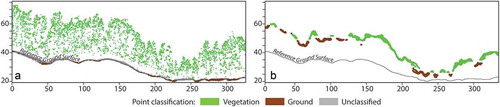
The density of the photogrammetric point cloud is based on the raster resolution of the photogrammetrically produced DSM (1 m). Thus, for this study the point density was 1 point/m², however this will vary with the resolution of the stereo imagery used to create the DSM. Although this density is similar to lidar point postings, the lidar point cloud’s multiple-return 3D structure enables the capture of both the top vegetation canopy and underlying canopy layers or the ground elevation, and results in multiple elevation (Z) values for each X,Y location in space. By comparison, the photogrammetric point cloud contains elevation values for only the top reflective surface of the imaged area. A cross section of the lidar point cloud is compared with that of the leaf-on photogrammetric point cloud (Figure 2). The photogrammetric point cloud captures either ground or vegetation elevations, resulting in large gaps in ground elevation measurement. The removal of non-ground elevation values from the photogrammetric point cloud eliminates any elevation measurement for the area they occupy, which necessitates interpolation from the closest points.

Figure 2. The 3D structure of the lidar point cloud (A) is inherently different than that of the photogrammetrically derived point cloud (B). Point classification using lidar techniques accurately identifies ground and vegetation points within the lidar dataset (A), but may not correctly differentiate between the two in the photogrammetrically derived dataset. Moreover, the elevation of vegetation point areas in the photogrammetric point cloud (B) must be interpolated from the closest ground point values.

This is quantitatively evident in comparison of the triangle facet areas of the TINs created from the ground returns of each dataset (Table 5). The larger mean area of TIN facets created from the ground points of the filtered photogrammetric DEMs (2.3 m² for WV1_FIL and 0.9 m² for WV3_FIL) compared with those of the lidar DEM (0.2 m²) indicates that both filtered photogrammetric DEMs have sparser ground measurements and thus require more interpolation. From this comparison, it is also evident that the ground points of the filtered leaf-on DEM (WV1_FIL) are sparser and thus require greater interpolation than those of the filtered leaf-off DEM (WV3_FIL).

Table 5. Area statistics for ground point TIN triangle facets.

Area metric (m^2)	Lidar ground points	WV1_FIL (leaf-on) ground points	WV3_FIL (leaf-off) ground points
Min	0.0	0.0	0.0
Maximum	262.3	1801.6	1575.3
Mean	0.2	2.3	0.9

There may be a vertical discrepancy between the elevations of photogrammetric “ground points” and elevations of lidar ground points (Figure 2). This is because the points may capture low areas in the vegetation canopy instead of the ground, and still fulfill the local height and planarity classification parameters for ground points in the photogrammetric point cloud. Although these photogrammetric “ground” points more closely resemble “low points in the vegetation canopy,” interpolation between them yields a DEM closer to the reference digital terrain model than either the original photogrammetric DSM or the SRTM.

Interpolated digital terrain models

All DEMs are shown planimetrically (Figure 3) using the same color ramp and linear 0–140 m stretch to allow for direct visual comparison of the reference DEM (Figure 3a) and SRTM (Figure 3b) to the photogrammetrically derived raw DSMs (Figure 3c and g) and filtered DSMs (Figure 3d–f and h). Profile visualization along a transect (Figure 4) allows for comparison of DEMs to the reference ground surface. Table 6 displays the results of the error assessment using descriptive statistics, normal distribution accuracy metrics and non-normal distribution accuracy metrics. All photogrammetric DEMs except the SRTM and WV3_DSM were found to have negative error skew, however most skewness values were close to 0 indicating only slight asymmetry in error value distribution. Notably, the WV3_DSM exhibited a strongly positive skew value of 4.91, and the WV3_FIL exhibited strongly negative skew value of −2.33. The strongly positive skew of the former indicates that the right (positive) tail of the distribution is long relative to the left (negative) tail, and suggests a higher frequency of positive errors. In the context of this research, a positive error value indicates that the elevation value of the tested DEM is higher than that of the NED. This situation is prevalent in both DSMs, where the presence of any above ground features causes elevations to result in positive errors when compared with a bare-earth digital terrain model. The strongly negative skew of WV3_FIL indicates that the left tail of the distribution is longer than the right tail. A negative error value indicates that the elevation value of the tested DEM is lower than that of the reference for a given location. This situation would arise in areas of interpolation, where the true ground surface rose and fell, but was not captured because the non-ground points were removed. The presence of skewness in these two DEMs suggests that non-normal distribution metrics, such as the 68.3 percentile value or NMAD should be evaluated in addition to the RMSE. Each DEM is discussed in additional detail in the following sections.

Figure 3. Visual comparison of DEMs: A) reference digital terrain map (from the NED); B) 30m SRTM; C) raw digital surface model from leaf on WV1 imagery (WV1_DSM); D) filtered DSM (WV1_FIL); E) filtered leaf on DSM with vertical offset for tall vegetation (WV1_FIL2); F) filtered leaf on DSM with vertical offset for near-stream points (WV1_FIL3); G) raw DSM from leaf off WV3 imagery (WV3_DSM); and H) filtered leaf-off DSM (WV3_FIL).

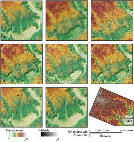
Figure 4. Profile comparison of DEMs. The map shows the transect location. The WorldView-1 Leaf-On DSM graph (top) compares the surface of WV1_DSM (green), WV1_FIL (red), WV1_FIL2 (yellow), and WV1_FIL3 (blue), with the reference DTM (black heavy line) and the SRTM (gray line). The WorldView-3 Leaf-Off DSM graph (bottom) compares the surfaces of WV3_DSM (red) and WV3_FIL (blue), with the reference DTM (black heavy line) and the SRTM (gray line) for the same transect.

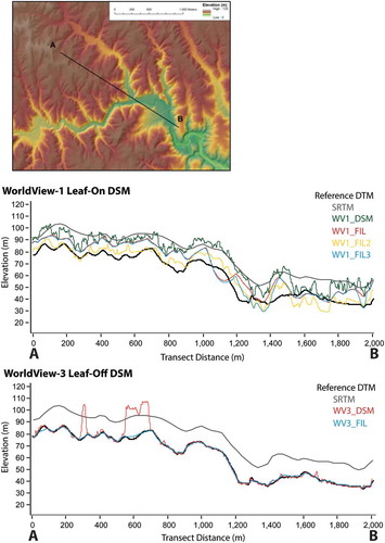
Table 6. Results of DEM error analysis.

		SRTM	WV1_DSM	WV1_FIL	WV1_FIL2	WV1_FIL3	WV3_DSM	WV3_FIL
Descriptive statistics
Signed error	Maximum (m)	26.62	28.77	22.13	17.07	22.19	25.61	4.47
	Minimum (m)	0.68	−16.77	−16.59	−22.53	−23.94	−4.90	−7.91
	Mean (m)	12.84	11.60	6.68	0.40	6.69	0.46	−0.71
	Std. dev (m)	4.11	7.25	6.94	6.90	7.19	3.77	1.05
	Skewness (m)	0.17	−0.66	−0.52	−0.43	−0.64	4.91	−2.33
Absolute error	Maximum (m)	26.62	28.77	22.13	22.53	23.94	25.61	7.91
	Minimum (m)	0.68	0.02	0.03	0.01	0.00	0.00	0.00
	Mean (m)	12.84	12.23	8.18	5.57	8.35	1.40	0.84
	Std. dev (m)	4.11	6.13	5.08	4.09	5.16	3.53	0.94
Normal distribution accuracy metrics
	RMSE (m)	13.48	13.68	9.63	6.91	9.82	3.79	1.26
	68.30rd percentile (m)	14.62	15.35	10.54	3.97	10.66	−0.05	−0.31
Accuracy metrics – no assumption of normality
	50th percentile (m)	12.76	12.42	7.18	1.00	7.19	−0.38	−0.56
	95th percentile (m)	19.70	22.30	17.09	10.74	17.29	3.87	0.45
	NMAD (m)	4.09	7.29	10.51	9.46	12.13	0.61	0.91

Descriptive statistics of signed error and absolute error, as well as normal distribution accuracy metrics and non-normal distribution accuracy metrics are given for each DEM evaluated in the study.

WV1_DSM

Although the raw leaf-on DSM (Figure 3c) captures the general topography of the study area, it is noisy and smooth terrain complexity compared with the reference. From the profile view (Figure 4), it is clear that the leaf-on WV1_DSM elevations generally lie between the reference DEM and the SRTM. Quantitative error metrics suggest that the WV1_DSM is comparable to the SRTM in accuracy. Its mean error of 11.60 m is slightly lower than the 12.84 m mean error of the SRTM, however its RMSE of 13.68 m is slightly higher than the SRTM’s 13.48 m RMSE. Of particular note, its non-normal distribution error values are greater than those of the SRTM (Table 6).

WV1_FIL

Simple removal of the non-ground points (method WV1_FIL) resulted in a DEM (Figure 3d) that qualitatively improved on the photogrammetric DSM. The large maximum positive error is comparable to that of the SRTM, but the minimum error is comparably large, indicating that some areas of the filtered DEM are below the reference surface. In evaluating terrain morphology of this filtered DSM, there are several high-elevation artifacts within the main stream valley caused by tall vegetation overhanging the stream. These artifacts function hydrologically as dams and would result in poor modeling of water flow. Bowl-shaped depressions in this DEM were caused by incorrectly classified ground point elevations (which should be vegetation) surrounding correctly classified ground point elevations, and indicate the limited success of this series of procedures.

Despite the presence of artifacts and outliers, these procedures decreased the error present in the DSM. Based on the low p-value result of the one-directional Wilcoxon test (Table 7), the null hypothesis is rejected and the median error value of WV1_FIL is found to be significantly (α < 0.05) less that of the unfiltered DSM, indicating the filtered DEM represents an improvement over the original data.

Table 7. Wilcoxon test of median error values.

	Estimated	Confidence interval (m)
DEM	median (m)	Lower	Upper
WV1_DSM	11.96	11.51	12.41
WV1_FIL	6.96	6.55	7.43
WV1_FIL2	0.66	0.22	1.10
WV1_FIL3	7.07	6.62	7.52

WV1_FIL2

The addition of a vertical offset to vegetation points (method WV1_FIL2) results in a DEM (Figure 3e) with minimum and maximum elevations similar to the reference DEM. However errors observed in the raw DSM and WV1_FIL are still present (albeit reduced). New errors have been introduced where the vertical offset overcompensated for vegetation height and pushed the filtered surface below the reference surface (Figure 4). Thus, while the WV1_FIL2 generally lies close to the reference surface, it exhibits several areas of “not sufficiently low” elevation, as well as areas of “too low” elevation.

Despite these inconsistencies, the WV1_FIL2 is quantitatively the most accurate leaf-on DEM (Table 6), with the lowest RMSE, mean error and non-normal distribution metric values. Based on the results of the one-directional Wilcoxon follow-up test (see Table 8), the null hypothesis is rejected and the median error value of WV1_FIL2 is found to be significantly less than that of both the unfiltered DSM and WV1_FIL.

Table 8. Wilcoxon one-directional test of median error values (less than the 11.96 m estimated median of WV1_DSM).

	Estimated	Wilcoxon	P-
DEM	median (m)	statistic	value
WV1_FIL	7.00	68507.0	0.000
WV1_FIL2	0.66	1439.0	0.000
WV1_FIL3	7.07	72591.0	0.000

WV1_FIL3

The inclusion of a vertical offset based on stream proximity (WV1_FIL3) produced a DEM (Figure 3f) with more terrain detail and a well-defined drainage pattern similar to the reference DEM. Qualitatively this method reproduced the terrain elements of the reference DEM (Figure 4), and improved the hydrologic functionality of the DEM. Despite these visual improvements, the RMSE, mean error, and non-normal distribution metric values for WV1_FIL3 are higher than those of WV1_FIL2 (Table 6). Furthermore, the Wilcoxon test results are somewhat contradictory for WV1_FIL3. The first test result (Table 8) indicates a rejection of the null hypothesis and confirms that the median value of WV1_FIL3 is significantly lower than that of the unfiltered DSM. However, the follow-up Wilcoxon test (Table 9) supports the acceptance of the null hypothesis that the median error of WV1_FIL3 is not significantly lower than that of the simple filtering (WV1_FIL). The latter result suggests that the simple vertical offset applied to all vegetation points of the WV1_FIL2 method produced a DEM with median error lower than that of the DEM with the more complex offset designed to improve hydrologic flow (WV1_FIL3).

Table 9. Wilcoxon one-directional test of median error values (less than the 6.995 m estimated median of WV1_FIL).

	Estimated	Wilcoxon	P-
DEM	median (m)	statistic	value
WV1_FIL2	0.66	40058.0	0.000
WV1_FIL3	7.07	253238.0	0.628

WV3_DSM and WV3_FIL

The leaf-off DEMs (Figure 3g and h) more successfully capture the range of elevation and complexity of terrain features visible in the reference DEM. Elevation artifacts caused by stands of evergreen vegetation are clearly visible in the raw leaf-off DSM (Figure 3g). These areas appear as contained areas of higher elevation than the surrounding terrain and are mostly removed by the filtering procedures (WV3_FIL). Qualitatively and quantitatively by all metrics, the filtered leaf-off DSM (Figure 3h) is the most similar to the reference DEM.

Effect of land cover on filtered DEMs

A positive correlation exists between canopy height and error in all leaf-on DSMs (Table 10), but the moderate strength of this relationship suggests that the magnitude of the difference between the DSMs and the ground is not entirely associated with the height of the vegetation canopy.

Table 10. Correlation coefficients for the error in each DEM (calculated as DEM minus NED) and the canopy height raster created from lidar.

DEM	Correlation coefficient
WV1_DSM	0.595
WV1_FIL	0.431
WV1_FIL2	0.486
WV1_FIL3	0.424
WV3_DSM	−0.053
WV3_FIL	−0.057

Results of the analysis of error by land cover class (Figure 5) indicates that error differs substantially by land cover. The difference in error between different land cover categories is greatest in the leaf-on DEMs, but even in the leaf-off DEMs error varies notably between the different land cover classes. It is not surprising that the leaf-on WV1_DSM reflects the largest difference in error values between land cover categories, as this DSM is created at a scale and during the phenological state that best captures canopy differences. However, it should not be assumed that the leaf-on DSM represents a perfect addition of the ground surface elevation and the height of vegetation canopy because the DSM does not consistently capture the upper canopy surface.

Figure 5. Error descriptive statistics for each DEM (m), presented by the land covers characterized in the land cover classification (see Appendix A). Analysis of error by these land cover classes is limited by the accuracies achieved in the classification (table A1).

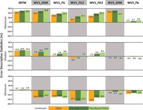
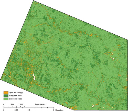
Figure A1. Land cover was classified into open areas, evergreen forest and deciduous forest by thresholding NDVI.

Comparison of DEMs by land cover is also important because it allows for the isolation of the open land cover category (Figure 5), which for all types of DEMs is conceptually equivalent to a bare-earth digital terrain model. Thus, evaluation of the median error within open areas compares the DEMs at their most accurate spots. In these areas of high accuracy, it can be seen that WV1_FIL3 has the lowest median error, and thus is the closest leaf-on DEM to the reference terrain. The additional procedures used to reduce vegetation height in WV1_FIL2 overcompensate for the elevations of above ground features, resulting in a negative median error. Both leaf-off DEMs (WV3_DSM and WV3_FIL) also have negative median error, but the value is substantially smaller than that of WV1_FIL2. Based on this median error metric, WV3_DSM has the lowest error and thus most closely models the reference terrain. The land cover class exhibiting the greatest potential error in each DEM is either deciduous forest or evergreen forest, depending on the seasonality of source imagery. In the leaf-on DEMs, median error of the filtered DEMs is lower for both deciduous and evergreen classes, suggesting that filtering successfully reduces the artifacts of vegetation canopy. Of these DEMs, WV1_FIL2 exhibits the smallest median error values. In the leaf-off DSM, median error is negative for both classes and increases as a result of filtering, but these values are small compared with those of the leaf-on DEMs.

Conclusion

This work evaluated how effectively classification and filtering procedures designed for lidar point clouds can be used to reduce the error in a photogrammetric DSM created from high-resolution stereo satellite imagery in a densely forested environment. As the methods investigated focus on a land cover context of predominantly forested area, the results may not be directly applicable in areas with many buildings. In such context, the central challenge in trying to generate a bare-earth DEM from photogrammetric methods is the lack of ground returns from beneath the vegetation canopy. In this study, fine spatial resolution photogrammetric DSMs were extracted from stereoscopic WorldView imagery in leaf-on and leaf-off conditions, then converted to a LAS point cloud. Ground terrain was identified using lidar point classification methods and then interpolated to create a bare-earth digital terrain model (DEM).

Overall it was found that a photogrammetric DSM, particularly one extracted from leaf-off imagery, may be processed to mitigate the effect of above ground features in the modeled elevation values, at a spatial resolution that preserves many of the terrain features visible in a bare-earth lidar DTM. However, the lack of multiple returns in the photogrammetric point cloud greatly limits the success of creating a bare-earth DTM in leaf-on forested land cover. Lidar processing techniques were partially successful in identifying points within the photogrammetric point cloud that fell on or near the ground surface, but the fundamentally different 3D structure of the point cloud ultimately limited their effectiveness. Filtering procedures substantially diminished the effect of the vegetation canopy on the DSM elevation surface, creating a DEM with an accuracy between that of the SRTM and a lidar bare-earth DEM. This filtered DEM would be useful for terrain visualization and estimation of elevation values, however it contains artifacts of the above ground features that limit its use in hydrologic modeling applications. Subsequent smoothing may reduce the effect of such artifacts and improve hydrologic flow, but at the cost of the fine-scale terrain detail.

Filtering procedures were more successful in removing the vegetation artifacts from the leaf-off photogrammetric DSM. In this study, the raw DSM extracted from leaf-off stereo imagery was similar in vertical accuracy to the reference DEM and correctly modeled the complexity of terrain features with minimal noise. Furthermore, elevation artifacts from evergreen vegetation and other above ground features were successfully removed using lidar filtering procedures, resulting in a bare-earth DEM with an accuracy comparable to that a bare-earth DEM created from lidar and useful for hydrologic modeling.

The findings of this study offer potential guidance for those considering the use of photogrammetric methods using high-spatial resolution imagery to generate DSMs in areas lacking high-resolution elevation data. The study area’s leaf-on, deciduous forestland cover presents a challenge for the creation of a bare-earth DEM, however the filtering procedures explored in this research significantly improved the accuracy and usability of each photogrammetric DSM. Additional research in this area should evaluate the potential of new filtering methods and point classification algorithms in different types of terrain and land cover, as well as the evaluation of these methods in areas where a lidar reference dataset is not available.

Disclosure statement

No potential conflict of interest was reported by the authors.

Appendix A

To facilitate a class-based evaluation of error, a land cover classification was carried out using the normalized difference vegetation index (NDVI) calculated from the monoscopic WorldView-3 multispectral imagery. The following classes were mapped: (1) open areas – including grass-covered fields, low-shrub areas such as power line corridors, and paved surfaces; (2) evergreen forest – including stands of pine and holly trees, and large shrubs such as rhododendron; and (3) deciduous forest. NDVI thresholds for these three classes were chosen based on a trial and error approach, and were, respectively, NDVI 0.3 < 1 standard deviation below the mean (0.57) for open areas; 1 standard deviation below the mean (0.57) < NDVI < the mean (0.67) for evergreen forest and NDVI > mean (0.67) for deciduous forest.

The resultant land cover map has an overall accuracy of 85%, based on stratified random sample of 475 points (Foody 2002). Table A1 shows the confusion matrix for the accuracy assessment, and the distribution of DEM evaluation points within each land cover is described in the results section.

Table A1. Confusion matrix for land cover classification. Overall accuracy is 85%.

		Reference image				User’s
		Field/open	Evergreen	Deciduous	Total	accuracy
Classified image	Field/open	14	4	14	32	44%
	Evergreen	4	67	50	121	55%
	Deciduous	6	39	277	322	86%
	Total	24	110	341	358
Producer’s accuracy		58%	61%	81%

References

- Axelsson, P. 1999. “Processing of Laser Scanner Data—Algorithms and Applications.” ISPRS Journal of Photogrammetry and Remote Sensing 54 (2–3): 138–147. doi:10.1016/S0924-2716(99)00008-8.H.
- Bühler, Y., M. Marty, and C. Ginzler. 2012. “High Resolution DEM Generation in High-Alpine Terrain Using Airborne Remote Sensing Techniques.” Transactions in GIS 16 (5): 635–647. doi:10.1111/j.1467-9671.2012.01331.x.
- Chirico, P. G., K. Malpeli, and S. Trimble. 2012. “Accuracy Evaluation of an Aster-Derived Global Digital Elevation Model (GDEM) Version 1 and Version 2 for Two Sites in Western Africa.” Giscience & Remote Sensing 49 (6): 775–801. doi:10.2747/1548-1603.49.6.775.
- Chu, H.-J., C.-K. Wang, M.-L. Huang, -C.-C. Lee, C.-Y. Liu, and -C.-C. Lin. 2014. “Effect of Point Density and Interpolation of Lidar-Derived High-Resolution Dems on Landscape Scarp Identification.” Giscience & Remote Sensing 51: 731–747. doi:10.1080/15481603.2014.980086.
- Dewberry. 2012. Project Report for the Virginia Counties North Acquisition and Classification for FEMA VA LiDAR.
- DeWitt, J. D., T. A. Warner, and J. F. Conley. 2015. “Comparison of DEMS Derived from USGS DLG, SRTM, a Statewide Photogrammetry Program, ASTER GDEM and Lidar: Implications for Change Detection.” Giscience & Remote Sensing 52 (2): 179–197. doi:10.1080/15481603.2015.1019708.
- Elmore, A. J., S. M. Guinn, and G. M. Sanders. 2013. Vegetation Structure within the National Capital Region Network Using Lidar Data and Analysis: Prince William Forest Park, Catoctin Mountain Park, C & O Canal National Historical Park, and Harpers Ferry National Historical Park.” Natural Resource Data Series. NPS/NCRN/NRDS—2013/475. Fort Collins, Colorado: National Park Service.
- Fisher, P. F., and N. J. Tate. 2006. “Causes and Consequences of Error in Digital Elevation Models.” Progress in Physical Geography 30 (4): 467–489. doi:10.1191/0309133306pp492ra.
- Gesch, D. B., M. J. Oimoen, and G. A. Evans. 2014. “Accuracy Assessment of the U.S. Geological Survey National Elevation Dataset, and Comparison with Other Large-Area Elevation Datasets – SRTM and ASTER.” U.S. Geological Survey Open-File Report 2014-1008: 10p. doi:10.3133/ofr20141008.
- Haala, N., H. Hastedt, K. Wolf, C. Ressl, and S. Baltrusch. 2010. “Digital Photogrammetric Camera Evaluation–Generation of Digital Elevation Models.” Photogrammetrie-Fernerkundung-Geoinformation 2010 (2): 99–115. doi:10.1127/1432-8364/2010/0043.
- Hofton, M., R. Dubayah, J. B. Blair, and D. Rabine. 2006. “Validation of SRTM Elevations over Vegetated and Non-Vegetated Terrain Using Medium Footprint Lidar.” Photogrammetric Engineering & Remote Sensing 72 (3): 279–285. doi:10.14358/PERS.72.3.279.
- Höhle, J., and M. Höhle. 2009. “Accuracy Assessment of Digital Elevation Models by Means of Robust Statistical Methods.” ISPRS Journal of Photogrammetry and Remote Sensing 64: 398–406. doi:10.1016/j.isprsjprs.2009.02.003.
- Kraus, K., and N. Pfeifer. 1998. “Determination of Terrain Models in Wooded Areas with Airborne Laser Scanner Data.” ISPRS Journal of Photogrammetry and Remote Sensing 53 (4): 193–203. doi:10.1016/S0924-2716(98)00009-4.
- Leberl, F., A. Irschara, T. Pock, P. Meixner, M. Gruber, S. Scholz, and A. Wiechert. 2010. “Point Clouds: Lidar versus 3D Vision.” Photogrammetric Engineering & Remote Sensing 76 (10): 1123–1134. doi:10.14358/PERS.76.10.1123.
- Maune, D. F. ed. 2007. Digital Elevation Model Technologies and Applications: The DEM Users Manual. Bethesda, MD: ASPRS Publications.
- Maxwell, A. E., and T. A. Warner. 2015. “Differentiating Mine-Reclaimed Grasslands from Spectrally Similar Land Cover Using Terrain Variables and Object-Based Machine Learning Classification.” International Journal of Remote Sensing 36 (17): 4384–4410. doi:10.1080/01431161.2015.1083632.
- Maxwell, A. E., T. A. Warner, and M. P. Strager. 2016. “Predicting Palustrine Wetland Probability Using Random Forest Machine Learning and Digital Elevation Data-Derived Terrain Variables.” Photogrammetric Engineering and Remote Sensing 82 (6): 437–447. doi:10.14358/PERS.82.6.437.
- Meng, X., N. Currit, and K. Zhao. 2010. “Ground Filtering Algorithms for Airborne Lidar Data: A Review of Critical Issues.” Remote Sensing 2 (3): 833–860. doi:10.3390/rs2030833.9iojhhjjkl.
- Mongus, D., and Ž. Borut. 2012. “Parameter-Free Ground Filtering of Lidar Data for Automatic DTM Generation.” ISPRS Journal of Photogrammetry and Remote Sensing 67 (1): 1–12. doi:10.1016/j.isprsjprs.2011.10.002.
- Montealegre, A. L., M. T. Lamelas, and J. De Riva. 2015. “A Comparison of Open-Source Lidar Filtering Algorithms in A Mediterranean Forest Environment.” IEEE Journal of Selected Topics in Applied Earth Observations and Remote Sensing 8 (8): 1–14. doi:10.1109/JSTARS.2015.2436974.
- Müller, J., I. Gärtner-Roer, P. Thee, and C. Ginzler. 2014. “Accuracy Assessment of Airborne Photogrammetrically Derived High-Resolution Digital Elevation Models in a High Mountain Environment.” ISPRS Journal of Photogrammetry and Remote Sensing 98: 58–69. doi: 10.1016/j.isprsjprs.2014.09.015. October 2015.
- Ni, W., K. J. Ranson, Z. Zhang, and G. Sun. 2014. “Features of Point Clouds Synthesized from Multi-View ALOS/PRISM Data and Comparisons with Lidar Data in Forested Areas.” Remote Sensing of Environment 149 : 47–57. Elsevier Inc.. doi:10.1016/j.rse.2014.04.001.
- Nortrup, M., and M. Lehman. 2013. “National Capital Region Network Resource Brief: Forest Structure & Lidar Imaging.” Part of National Capital Region Inventory and Monitoring Program. Tech. Rep. NPS/NCRN/NRDS-2010/043. Fort Collins, CO: National Park Service.
- Ressl, C., B. Herbert, G. Mandlburger, and N. Pfeifer. 2016. “Dense Image Matching Vs. Airborne Laser Scanning – Comparison of Two Methods for Deriving Terrain Models.” Photogrammetrie-Fernerkundung-Geoinformation 2016 (2): 57–73. doi:10.1127/pfg/2016/0288.
- Sefercik, U. G., M. Alkan, G. Buyuksalih, and K. Jacobsen. 2013. “Generation and Validation of High-Resolution Dems from Worldview-2 Stereo Data.” Photogrammetric Record 28 (144): 362–374. doi:10.1111/phor.12038.
- Sithole, G., and G. Vosselman. 2004. “Experimental Comparison of Filter Algorithms for Bare-Earth Extraction from Airborne Laser Scanning Point Clouds.” ISPRS Journal of Photogrammetry and Remote Sensing 59 (1): 58–101. doi:10.1016/j.isprsjprs.2004.05.004.
- Tarolli, P. 2014. “Geomorphology High-Resolution Topography for Understanding Earth Surface Processes: Opportunities and Challenges.” Geomorphology 216: 295–312. doi:10.1016/j.geomorph.2014.03.008.
- Toutin, T. 2004. “Review Article: Geometric Processing of Remote Sensing Images: Models, Algorithms and Methods.” International Journal of Remote Sensing 25 (10): 1893–1924. doi:10.1080/0143116031000101611.
- Wohlfeil, J., H. Hirschmüller, B. Piltz, A. Börner, and M. Suppa. 2012. “Fully Automated Generation of Accurate Digital Surface Models with Sub-Meter Resolution from Satellite Imagery.” International Archives of the Photogrammetry, Remote Sensing and Spatial Information Sciences 34-B3: 75–80.
- Wolf, P. R., B. A. Dewitt, and B. E. Wilkinson. 2014. Elements of Photogrammetry with Applications in GIS. Fourth ed. New York: McGraw-Hill Education.