A comparison of geographic datasets and field measurements to model soil carbon using random forests and stepwise regressions (British Columbia, Canada)

Abstract

We used geographic datasets and field measurements to examine the mechanisms that affect soil carbon (SC) storage for 65 grazed and non-grazed pastures in southern interior grasslands of British Columbia, Canada. Stepwise linear regression (SR) modeling was compared with random forest (RF) modeling. Models produced with SR performed better than those produced using RF models (r² = 0.56–0.77 AIC = 0.16–0.30 for SR models; r² = 0.38–0.53 and AIC = 0.18–0.30 for RF models). The factors most significant when predicting SC were elevation, precipitation, and the normalized difference vegetation index (NDVI). NDVI was evaluated at two scales using: (1) the MOD 13Q1 (250 m/16-day resolution) NDVI data product from the moderate resolution imaging spectro-radiometer (MODIS) (NDVI_MODIS), and (2) a handheld multispectral radiometer (MSR, 1 m resolution) (NDVI_MSR) in order to understand the potential for increasing model accuracy by increasing the spatial resolution of the gridded geographic datasets. When NDVI_MSR data were used to predict SC, the percentage of the variance explained by the model was greater than for models that relied on NDVI_MODIS data (r² = 0.68 for SC for non-grazed systems, modeled with SR based on NDVI_MODIS data; r² = 0.77 for SC for non-grazed systems, modeled with SR based on NDVI_MSR data). The outcomes of this study provide the groundwork for effective monitoring of SC using geographic datasets to enable a carbon offset program for the ranching industry.

Keywords:

• Normalized difference vegetation index (NDVI)
• remote sensing
• random forest
• carbon sequestration
• climate change

1. Introduction

Rising greenhouse gas levels intensify the processes driving climate change, threatening to alter ecosystem structure and properties at a global scale (Hansen 2008). Grasslands may be affected by these intensified processes through drought and erosion, decreased biodiversity, and ecosystem degradation (Winslow, Hunt, and Piper 2003). Land use changes have simultaneously resulted in the depletion of soil carbon (SC) levels, releasing carbon (C) from the soil into the atmosphere. This depletion is largely the result of reduced plant root material and residues being returned to the soil, increased decomposition from soil tillage, and increased soil erosion (Lal 2004; Wall, Nielsen, and Six 2015). Depletion of SC stocks may be remediated through an assortment of improved land management approaches. SC sequestration – the process of storing C in the soil through crop residues and other organic solids – has been an area under much investigation as it relates to reducing atmospheric CO₂ and mitigating climate change. Soils with high C content are also associated with increased fertility, water retention, and vegetation productivity (Victoria et al. 2012).

Since grasslands predominately sequester C below ground through root networks and the inherent soil-building processes, carbon is deposited beneath the surface in relatively stable forms. For this reason, grasslands have a high potential for long-term SC storage and therefore are of major importance for maintaining Earth’s C cycle (Parton et al. 1995; McSherry and Ritchie 2013; Zhou et al. 2016). The process of C sequestration relies on respiration and photosynthesis by vegetation, two basic processes of the C cycle. Carbon may also enter the soil in the form of litter, harvest residues, and animal manure. These inputs also contribute to the SC sink and are stored as soil organic matter. In many areas, poor land use management can upset this process, thereby causing a net emission of C. The rate at which carbon is sequestered in soil is dependent on many environmental factors (e.g., climate and landscape) and management practices (e.g., cattle grazing).

1.1. Using vegetation indices to model SC

The abundance of organic C in the soil affects and is affected by plant growth. Specifically, plant productivity, shoot/root allocation, and vertical root distribution by different functional groups (e.g., grasses, shrubs, trees) can influence the depth of soil organic carbon (SOC) contributions (Jobbágy and Jackson 2000). Also, the presence of perennial grass and legume species was a key cause of greater soil C and N accumulation in both higher and lower diversity plant assemblages because legumes have unique access to N, and C4 grasses take up and use N efficiently, increasing below-ground biomass and thus soil C and N inputs (Fornara and Tilman 2008). Vegetation Indices (VIs) are combinations of surface reflectance at two or more wavelengths designed to highlight a property of vegetation, and they are commonly used as a surrogate for plant biomass. Recently, remote sensing (RS) has been used to predict SC by modeling methods that employ VIs as inputs. The distribution of SC has been shown to be highly correlated with the normalized difference vegetation index (NDVI), and piecewise regression tree modeling using 2 m NDVI data acquired by the IKONOS satellite combined with weather and net ecosystem production performs well (r = 0.88) for predicting SC (Zhang et al. 2012).

1.2. Other factors affecting SC

1.2.1. Climate and topography

The environmental variables that influence SC are often interconnected and relate to the productivity and stability of a landscape. Conant and Paustian (2002) modeled potential SC sequestration in overgrazed grassland ecosystems and established a positive linear relationship between potential SC sequestration and mean annual precipitation (MAP). The regression model predicted losses of SC with decreased grazing intensity in drier areas (MAP<333 mm/year) but substantial sequestration in wetter areas, though most (93%) of the C sequestration potential was predicted in areas with MAP less than 1800 mm (Conant and Paustian 2002). Sumfleth and Duttmann (2008), on the other hand, showed that elevation was the most important predictor of SC in Chinese agricultural fields, though soil moisture was mentioned as a predictor of lower importance. However, elevation and soil moisture are likely to be highly correlated in some geographical contexts, and for this reason, we expect that aspect and elevation may also be useful indicators of SC, since low-lying south facing slopes are typically drier. Furthermore, since areas on steeper slopes may be more likely to experience erosion, we expect steep slopes to help indicate regions with low SC.

1.2.2. Soil properties

Soil types indicate differences in many soil characteristics including organic matter content, drainage, litter production, and soil texture. These characteristics influence SC directly and indirectly by affecting productivity, drainage, and stability. A study by Bhatti, Apps, and Tarnocai (2002) has successfully used soil classifications to improve the performance of predictive SC models. Specifically, the SC predictions were based on data from (1) analysis of pedon data from both the Boreal Forest Transect Case Study area and from a national-scale soil profile database; (2) the Canadian Soil Organic Carbon Database (CSOCD), which uses expert estimation based on soil characteristics; and (3) model simulations with the Carbon Budget Model of the Canadian Forest Sector (CBM-CFS2) (Bhatti, Apps, and Tarnocai 2002).

The impact of soil type on SC, however, is interrelated with the effect of precipitation. The effect of this interrelation can be either to increase or decrease the SC, depending on the soil type. In their recent study, McSherry and Ritchie (2013) showed that an increase in MAP of 600 mm resulted in a 24% decrease in “grazer effects” on SOC for finer textured soils, while the same increase in precipitation over sandy soils produced a 22% increase in “grazer effects” on SOC.

1.2.3. Cattle grazing

Although the negative effects of overgrazing are well documented, there is controversy regarding potential benefits of more conservative grazing practices. Overgrazing can lead to poor range health and reduce the potential for rangelands to sequester C in the soil (Chapman and Lemaire 1993; Zhou et al. 2016), and it is widely accepted that overgrazing is detrimental to plant communities due to selective and repetitive defoliation and trampling, which can lead to a loss in species diversity, reduced vegetation biomass and density, and an increase in undesirable non-native invasive plants which thrive in disturbed ecosystems (Chapman and Lemaire 1993). Grazing may also affect hydrology and soil properties, such as increased soil erosion, reduced water infiltration and soil compaction, and lower soil quality and fertility (Schlesinger 1999; Bremer et al. 2001). However, recent studies suggest that light-to-moderate grazing may serve to increase soil building processes and SC storage by increasing compensatory growth of forage species and turnover of plant roots, and better facilitating soil development (Loeser, Sisk, and Crews 2007; Schönbach et al. 2011; Zhou et al. 2016). Similarly, light grazing may also improve shoot turnover compared to fenced, non-grazed conditions (Schuman et al. 1999). Furthermore, aboveground immobilization of C in standing dead plant material in non-grazed areas may lead to lower levels of observed SC (Schuman et al. 1999).

Schuman et al. (1999) found that 12 years of season-long cattle grazing at 0.67 and 2 animal unit months per hectare resulted in significant increases of 21% and 22% of the total SC, respectively, relative to non-grazed pasture. This increase in SC under grazed conditions was attributed to the increase in blue grama cover, a species which is known to develop a dense and continuous root mass in the upper soil layer and allocate more C and nutrients to roots than other species commonly found in the mixed-grass prairie. Conant and Paustian (2002) also noted the positive impact of blue grama cover for increasing SC under grazed conditions. This study also concluded that most C sequestration was located in areas that were lightly or moderately grazed, while only a small amount was located in strongly grazed grasslands (Conant and Paustian 2002). The conflicting results of previous studies on the effects of grazing on SC have been attributed to the fact that SC dynamics are highly context specific and their causations are interrelated (McSherry and Ritchie 2013).

1.3. Objectives

This study evaluates the factors which influence SC in temperate grassland ecosystems using stepwise linear regression (SR) and random forest (RF) modeling and to use these models to map SC throughout the temperate grasslands of British Columbia (BC), Canada. We have evaluated the importance to the SC prediction of several factors that influence SC content: (1) grazing; (2) climate; (3) landscape variables including aspect, soil, and elevation; (4) NDVI; (5) vegetation community zones; and (6) soil type classifications. Grazing density information is not generally available at the regional scale (such as the Province of British Columbia) and thus was not included as a potential predictor variable in the models. Instead, separate models were developed for areas that were fenced to exclude grazing and for areas where grazing occurred. These models were compared to determine if grazing impacted the set of predictor variables selected during the modeling process. Furthermore, we compare the use of a satellite-acquired NDVI product with field-radiometer acquired NDVI measurements for modeling SC to explore the potential for increasing model accuracy by increasing the spatial resolution of the gridded geographic datasets. The MOD 13Q1 (250 m/16-day resolution) NDVI data product from the moderate resolution imaging spectro-radiometer (MODIS) was selected because these data are freely available and cover the spatial and temporal range of our study area. For field-radiometry, we used a Cropscan, Inc. MSR16R multispectral radiometer (MSR) to produce NDVI measurements with a spatial resolution of 1 m (NDVI_MSR). This study lays the groundwork for effective monitoring techniques of SC levels using RS methods that could lead to the possibility of a carbon-offset program for the ranching industry.

2. Materials and methods

2.1. Study area

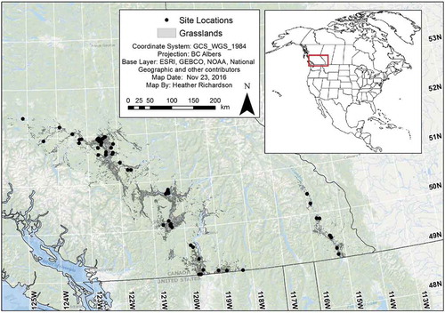
The study area is located in temperate grasslands of the southern interior of BC. To capture the climatic, topographic, and vegetative differences throughout these grasslands, 65 sites were sampled (Figure 1; see Appendix A for a list of site locations, code names, and coordinates). To evaluate the effect of long-term grazing, samples were taken at non-grazed range reference areas (RRA), which are permanent fencing installations (i.e., exclosures) used to monitor the impact of livestock on BC rangelands. Among the sites, elevation ranges from 346 to 1213 m above mean sea level and MAP ranges from 302 to 538 mm/year.

Figure 1. Sample site locations of range reference areas within the grassland of the south-central interior of British Columbia, Canada. For full colour versions of the figures in this paper, please see the online version.

2.2. Sampling

At each RRA, two 5 m × 5 m sampling plots were established: in grazed (outside a fenced exclosure) and non-grazed (inside a fenced exclosure) areas. In each plot, five 30 cm deep holes were augured. At two of the five holes, all excavated soil was removed for bulk density analysis. SC samples were taken from each of the five holes by scraping soil from the sidewall at the following depth increments: 0–10, 10–20, 20–30 cm. Vegetation cover class and dominant vegetation species were recorded within each 5 m × 5 m plot; however, this data were not used for modeling because the vegetation data did not exhibit a strong correlation with the measured SC and because there is no equivalent geographic dataset available for areas not included in our field campaign. Instead, these data were used to estimate the vegetation community of the sampling plot. For the predictive modeling, the vegetation community was derived from a geodataset published by the Grasslands Conservation Council of BC (see Section 5.4). During field sampling, photos were taken and landscape variables were measured (slope with clinometer, elevation with GPS, aspect by sight). During the second field season, a data logger controller MSR (MSR16R, CROPSCAN Inc.) was used to determine spectral reflectance of the land surface (five replicates per site). The MSR16R measures reflectance in 16 spectral bands throughout the 450–1750-nm region. Data collected from this device were later used to calculate NDVI readings using the following equation:

(1)

where NIR and RED are reflectance values for wavelengths within the near-infrared spectrum and the red-light spectrum, respectively. The NIR and RED reflectance values were measured using bands centered at 830 and 650 nm, respectively.

2.3. SC analysis

To measure the SC content for each of the 5 m × 5 m sampling plots, the soil samples were dried, sifted through a 2-μm sieve, and weighed on an analytical scale before analysis through an automated elemental analyzer (CE-440 Elemental Analyzer, Exeter Analytical Inc.), which determined C percent by thermal conductivity detection. Three of the five samples were run through the analyzer individually (not bulked). The inter-sample variance was usually quite low; however, if the inter-sample variance was unusually large, the additional two samples were run as well.

2.4. Data

Several datasets were used to model and map SC (Table 1). The MOD 13Q1 data tiles which comprise the NDVI_MODIS dataset required significant preprocessing. This preprocessing was performed using R (version 3.0.2) (R Development Core Team 2016) and included the following processing steps. First, the appropriate tiles were downloaded, projected in to the BC Albers Equal Area projection, and mosaicked into BC-wide gridded geodatasets. A mosaic was produced for each 16-day composite, resulting in 69 layers for the 2011–2013 time period. To reduce noise in the NDVI_MODIS data, caused primarily by cloud contamination and atmospheric variability, the NDVI_MODIS datasets were temporally ordered and smoothed by a pixel-by-pixel computation of NDVI_MODIS values over the 3-year time series using Loess smoothing. All other geodatasets were preprocessed using Model Builder in ArcGIS (version 10.1). This preprocessing included projection of the data into BC Albers Equal Area projection, and since the data values exhibited positive skew, they were transformed to log-normal using ln(value + 1). The “+1” was used because some of the original data had values of zero, which would have caused an error when the log function was evaluated.

Table 1. GIS for soil carbon modeling and mapping.

Layer name	Description (year created)	Format (resolution)	Publisher
MAP	The average annual precipitation in millimeters for the period 1961 to 1990 (2005)	Raster (2.5 arc min) (approx. 5 km)	Ministry of Forests and Range, Research Branch
MAT	The average temperature for the entire year in degrees Celsius for the period 1961 to 1990 (2005)	Raster (2.5 arc min) (approx. 5 km)	Ministry of Forests and Range, Research Branch
Soil type	Soil Development type derived from Soil Landscapes of Canada data (2008)	Vector	Agriculture and Agri-Food Canada
Soil drainage	Describes the removal of water from the soil, derived from Soil Landscapes of Canada data (2008)	Vector	Agriculture and Agri-Food Canada
Vegetation community	Vegetation community zones derived from Biogeoclimatic Ecosystem Classification zones (2004)	Vector	Grasslands Conservation Council of British Columbia
Aspect, slope, elevation	Topographic layers derived from gridded DEM created by the TRIM program (2002)	Raster (30 m)	Base Mapping and Geomatic Services
NDVIMODIS	Satellite derived Normalized Difference Vegetation Index data (16 days/250-m resolution) from Moderate-resolution Imaging Spectro-radiometer (MODIS) satellite, MOD13Q1 product (2012–2014)	Raster (250 m)	USGS, MODIS Terra Land Processes Distributed Active Archive Center directory

TRIM: Terrain Resource Information Management.

2.5. Statistical analysis

The study design allowed for paired t-tests to compare grazed and non-grazed data from 2013 and 2014. All analyses were performed using R (version 3.0.2) (R Development Core Team 2016) and the R package “car” (Fox and Weisberg 2011).

2.6. Modeling and mapping

Data were randomly divided into training and testing data. Two-thirds of the sites were assigned as training data (n = 43) and one-third was assigned as validation data (n = 22). All factors affecting SC levels were evaluated simultaneously through RF and SR modeling, using the training data. The models were validated by predicting outcomes for the validation dataset and comparing with the observed data, to calculate a mean squared error (MSE) value. The best SR models were selected automatically via forward–backward stepwise regression with the “step” function in R (Venables & Ripley, 2002), which defines model fitness as low Akaike information criterion (AIC) and high coefficient of determination (r²) values. The RF modeling method, using the “randomForest” package in R (Liaw and Wiener, 2002), constructs a model by sequentially evaluating the set of input variables based on the reduction in model performance (evaluated as MSE) when each of the variables is perturbed. Using this sensitivity analysis, variables are sequentially added to the model until no further improvements in the model performance can be made by adding additional terms. The final models were compared using the r², MSE, and AIC fitness measures. To compare AIC between model types, the AIC of each model was computed manually using the modified AIC equation by Hastie, Tibshirani, and Friedman (2001):

(2)

where s² is the squared sum of variance between the predicted and actual values of the test dataset (N) and d is the number of parameters. For SR, d is equal to the number of variables in the output model plus 2 for the variance and intercept, respectively. For RF, d is calculated as

(3)

where 1 is added for the variance. The average number of times the variables are used in one tree of the forest was determined with the “varUsed” function of the randomForest package (Liaw and Wiener, 2002 ), which calculates the amount of times each variable was used in the RF. These values were summed and divided by the number of trees in the forest (501).

Since running BC-wide calculations in R is extremely time consuming, the predictive maps created with SRs were generated with Model Builder in ArcGIS while the predictive maps created with RF models were generated in R using the RF “predict” function. With Model Builder, Raster Calculator was used to predict SC based on the stepwise regression equations. Finally, predictive maps were clipped to the extent of the BC grasslands, as defined by a geodataset created by the Grasslands Conservation Council.

Mapping was performed using R packages “rgdal” (Bivand et al., 2015), “raster” (Hijmans, 2015), and “XML” (Lang and the CRAN Team, 2016) (R Core Team 2016) and ArcGIS (version 10.1) (ESRI 2012).

3. Results

3.1. SC in grazed versus non-grazed areas

A paired t-test on SC content measured inside and outside fenced RRAs in our study area, which prevented cattle grazing within the fenced area, indicated that there were no significant differences in SC between grazed areas versus non-grazed (p = 0.614) at soil depths of 0–10 cm.

3.2. Change in SC over time

From 2013 to 2014, the average SC increased by 0.12% from 1.35% to 1.47% based on a paired two-sample t-test. The null hypothesis of this test was that the 2013 SC was greater or equal to the 2014 SC and was rejected at a 5% level (p = 0.001).

3.3. Stepwise regression and RF models

Two separate sets of SR and RF models were created, one for NDVI_MODIS (grazed and non-grazed) and the other for NDVI_MSR (grazed and non-grazed). Both modeling procedures drive model creation by evaluating which factors out of a set of potential factors significant predictors of SC. When the NDVI was based on MODIS-acquired data, SR selected NDVI_MODIS, elevation, and MAP as important predictors of SC in both grazed and non-grazed plots. While for the models constructed using MSR-derived NDVI, SR selected NDVI_MSR, soil type, and vegetation community as important predictors of SC in grazed sites and NDVI_MSR and vegetation community as important predictors of SC in non-grazed areas. Table 2 summarizes these models and provides measures of their predictive performance. NDVI measured by the MSR (NDVI_MSR) produced the most accurate models, explaining 70% and 77% of the variance in the observed SC data for grazed and non-grazed plots, respectively. In contrast, NDVI measured by the MODIS (NDVI_MODIS) explained 56% and 68% of the variance in the observed SC data for grazed and non-grazed plots.

Table 2. Stepwise regression for 2014 soil carbon in grazed and non-grazed systems comparing Normalized Difference Vegetation Index derived from MODIS (NDVI_MODIS) and the multispectral radiometer (NDVI_MSR).

	NDVIMODIS				NDVIMSR
	Grazed		Non-grazed		Grazed		Non-grazed
	Est	Sig	Est	Sig	Est	Sig	Est	Sig
Intercept	−15.86	***	−13.50	***	−13.05	***	−8.67	**
Elevation	1.31	***	1.11	***	0.67	.	0.42	..
Aspect					0.13	..
Slope
MAT	0.75	..	0.50	..
MAP	1.02	*	0.99	**	1.28	*	0.96	**
NDVIMODIS	2.05	.	1.74	*	NA	NA	NA	NA
NDVIMSR	NA	NA	NA	NA	2.96	***	3.33	***
Soil type					0.44	*
Soil drainage							0.28	..
Veg community			−0.14	..	−0.37	**	−0.30	**
r^2	0.56		0.68		0.70		0.77
MSE	0.11		0.13		0.16		0.09
AIC	0.29		0.23		0.30		0.16

The coefficients (Est) and significance (Sig) of each variable in the model is displayed. Sig: significance codes of p values represented by ***: <0.0001, **: <0.001, *: <0.01, ..: <0.05, .: <0.1.

The RF models for 2014 are summarized in Table 3. These models are similar to the SR models in terms of the set of predictor variables they include. Using MODIS-derived NDVI, RF model selected the variables MAP, NDVI_MODIS, slope, vegetation community, and drainage as important predictors of SC in both grazed and non-grazed plots. The RF model for grazed plots explained 38% of the variance in the observed SC data while the RF model for non-grazed conditions explained 53% of the variance in the observed SC data. Using MSR-derived NDVI, RF modeling identified NDVI_MSR, MAP, and vegetation community as important predictors of the SC in grazed areas and NDVI_MSR, vegetation community, and slope as important predictors of the SC in non-grazed areas. The models using MSR-derived NDVI explained 38% and 44% of the variance in the observed SC for grazed and non-grazed plots, respectively.

Table 3. Random forest for 2014 soil carbon in grazed and non-grazed systems comparing normalized difference vegetation index derived from MODIS (NDVI_MODIS) and the multispectral radiomete(NDVI_MSR).

	NDVIMODIS		NDVIMSR
	Grazed	Non-grazed	Grazed	Non-grazed
Elevation	15.13	16.24	19.55	18.57
Aspect
Slope	4.72	7.59		4.06
MAT
MAP	7.55	8.79	7.95
NDVIMODIS	6.08	12.88	NA	NA
NDVIMSR	NA	NA	7.33	5.83
Soil type
Soil drainage	0.69	1.14
Veg community	4.06	6.22	4.56	7.55
r^2	0.38	0.53	0.38	0.44
MSE	0.11	0.13	0.07	0.10
AIC	0.27	0.30	0.18	0.23

Results show “%incMSE,” the percent increase in mean square error when variable is permutated. Variables with negative “%incMSE” values were removed from the model and therefore not displayed in the table.

Based on comparisons of the r² and AIC goodness-of-fit measures, SR produces models that explain more of the variance in the observed SC data and are more efficient than the RF models (r² = 0.49–0.77 and AIC = 0.30–0.13 vs. r² = 0.36–057 and AIC = 0.36–0.18) (Tables 2 and 3), and six of the eight SR models have higher r² and lower AIC values in comparison to the RF models (Tables 2 and 3).

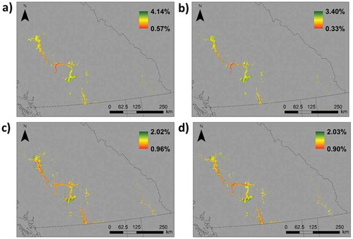
Maps of the predicted 2014 SC throughout the grasslands of BC’s southern interior based on both the SR and RF models developed for grazed and non-grazed conditions are illustrated in Figure 2. Visually analysis of these maps reveals that both modeling methods produce similar spatial patterns, despite the SR models explaining a greater proportion of the variance in the observed SC data.

Figure 2. Predicted soil carbon (SC) percentage in the top 10 cm of the soil column based on stepwise regression (SR) and random forest (RF) models: (a) SR grazed 2014, (b) SR fenced (non-grazed) 2014, (c) RF grazed 2014, (d) RF fenced (non-grazed) 2014.

4. Discussion

This study examined the relationships between several geographic variables and SC at 65 grazed and non-grazed pasture sites within southern interior grasslands of BC. The results of this study reveal insight into the impact of cattle grazing on SC, as well as the feasibility of modeling SC at the regional scale.

4.1. Impact of cattle grazing on SC

Our data did not reveal a statistically significant difference between the grazed and non-grazed areas, a result which suggests that the variance between geographic locations was of the same magnitude or larger than the variance between grazed and non-grazed treatments. However, the models developed to predict SC in grazed areas were found to rely on a different set of predictor variables than the models developed to predict non-grazed areas (Tables 2 and 3). Although grazer effects are clearly important to predicting SC, the modeling performed in this study did not consider grazing intensity as a predictor variable, because these data are seldom available at the regional-scale investigated in this study. Instead, models were created for both grazed and non-grazed conditions. Although this modeling decision limits our ability to interpret the impact of grazing on SC sequestration from the resulting models, we are still able to draw the following conclusions: (1) cattle grazing at the levels present at our study sites does not result in significant differences in the measured amount of SC at a particular location, and (2) cattle grazing impacts the geographic characteristics that best predict SC. Taken together, these two results suggest that SC may be more variable between sites than between grazing treatments (grazed or non-grazed samples at a single site), and that grazing may serve to either increase or decrease SC depending on local conditions, an idea also suggested by McSherry and Ritchie (2013). In fact, the combined effects of site variability and grazing may serve to amplify or dampen the overall trends observed in SC, and therefore, we must examine the differences in the models of grazed and non-grazed systems to identify in what contexts grazing increases or decreases C storage.

Comparison of the models developed for both grazed and non-grazed conditions revealed that grazing changed the influence of landscape characteristics as predictors of SC. In grazed sites, MAP, soil type, and aspect were stronger predictors of SC than in non-grazed sites. While Conant and Paustian (2002) developed a model that showed losses of SC with decreased grazing intensity in drier areas (MAP < 333 mm/year) and substantial sequestration in wetter areas, though 93% of C sequestration potential occurred in areas with MAP less than 1800 mm/year, our models suggest that there are additional landscape features that interact with grazing and precipitation to influence SC storage. However, many previous studies have shown that grazing can have both a strong positive and negative impact on SC (Schlesinger 1999; Chapman and Lemaire 1993; Schuman et al. 1999; Bremer et al. 2001; Loeser, Sisk, and Crews 2007; Schönbach et al. 2011; Evans et al. 2012; Krzic et al. 2014; McSherry and Ritchie 2013; Zhou et al. 2016). Due to these contradicting studies, it is difficult to quantify how grazing might impact SC at a given site.

Despite these contradictions, however, studies agree that there is potential for additional C storage in grasslands. Indeed, our research showed that from 2013 to 2014, the average SC increased by 0.12% from 1.35% to 1.47%, though this change may be in the range of inter-annual variability and a longer term time series would be necessary to determine a more robust estimate of the long-term SC trend. Thompson et al. (2008) modeled the potential rate of C sequestration by three ecosystem types over a period of 100 years and concluded that agricultural lands have the potential to store 0.21 GtC/year, reforested lands store 0.31 GtC/year, and pasture lands have the potential to store 0.15 GtC/year. Conant et al. (2001) estimated that, under different management scenarios, grassland ecosystems have the capacity to sequester up to 0.54 MgC/year per hectare. This suggests that the grasslands of BC’s southern interior have the potential to store additional C and thus contribute to climate change mitigation through atmospheric GHG reductions.

There is great interest in the concept of mitigating climate change through the removal of CO₂ from the atmosphere by sequestering C within the soil. Studies examining other regions have shown rehabilitation of rangelands to effectively mitigate C emissions in other regions (Dean, Wardell-Johnson, and Harper 2012); however, it can be expensive to alter land management practices. The development of a C offset program for ranchers may be incentive to employ sustainable practices, compensating ranchers for providing the valuable ecosystem service of C sequestration.

4.2. Using VIs to model SC

The modeling performed in this study showed that NDVI is an important predictor of SC and that the spatial support (i.e., the spatial averaging area) of the NDVI value used as a predictor has significant impacts on the performance of the derived model. Past research has shown that the distribution of SC is correlated with NDVI and other VIs (e.g., the enhanced vegetation index, EVI) computed from RS data (Zhang et al. 2012; Yang and Mouazen 2012), and our results suggest that the degree of correlation between NDVI and SC is influenced by the spatial support of the NDVI measurement. When NDVI_MSR data were substituted for NDVI_MODIS in the SC model, the model’s performance, in terms of r² and MSE, increased. Since the NDVI_MODIS product used in this work has a resolution of 250 m, it is likely that each raster pixel contains both grazed and non-grazed areas as well as significant spatial variability in the landscape characteristics. Thus, it is logical that predictive models of SC based on the much higher resolution (1 m) NDVI_MSR data performed better than those models based on the NDVI_MODIS data product. The impact of spatial support of the NDVI measurements on the performance of predictive models of SC has also been noted by Gomez, Rossel, and McBratney (2008). This study investigated models that relied only on spectral measurements to predict SC and showed that the performance of such models based on measurements from an Agrispec field spectrometer (similar to the MSR used in this study) outperformed models based on measurements from the Hyperion hyperspectral satellite remote sensor (30-m resolution), although not by a large margin. Field-based spectral measurements, however, cannot be collected for mapping SC across vast areas, and instead, the predictive models used for the mapping must be based on RS acquired from airborne platforms, including both satellite and aircraft. The recent emergence of spectrometer equipped unmanned aerial vehicles (UAVs) may play an increasingly important role, as they can operate in remote areas and provide very-high (submeter) resolution spectral measurements (Hill et al. 2016; Feng, Liu, and Gong 2015).

4.3. Comparison of stepwise regression and RF models

In our comparison of SR and RF, SR appears to be the better tool for modeling SC in unmeasured areas of BC grasslands because they performed better while having less complexity than the RF models and because they are more easily interpreted. Based on the r² and AIC goodness-of-fit measures, SR generally produced better models for predicting SC at unmeasured locations than RF. We found this result surprising because more complex models, such as RF, have been shown to perform better in general than simpler models, such as stepwise regression, for digital soil mapping (Brungard et al. 2015). Additionally, since an RF model is composed of many regression trees, this type of model is more challenging to interpret than a SR model. This latter point is important if the models are to be analyzed to facilitate understanding of the processes that govern SC sequestration, an important first step for driving economic models of carbon stocks and enabling land use management.

4.4. The novelty and limitations of our approach

This research has developed models based on readily available data coverages to predict SC at the regional scale. NDVI imagery derived from the MODIS sensor is updated every 16 days at a 250-m resolution and was found to be an important predictor variable in our models. Since models based on NDVI_MODIS do not require field measurements, SC can be predicted throughout BC’s grasslands without laborious field campaigns. Therefore, the outcomes of this work serve as the first step toward a SC monitoring program in grasslands, because the models developed here can be updated as more current remotely sensed data become available.

Despite the successes of this work, there are three limitations that should be addressed before the modeling framework developed in this study could be used to drive a carbon offset program for ranchers. The first of these limitations is that our field sampling method was not able to retrieve soil samples throughout the entire soil column. Because our sampling areas were located at RRAs, which are protected from disturbance, we were restricted from creating soil pits to collect our soil samples and required to minimize our disturbance to the soil. For this reason, we used an auger to drill a 20-cm wide hole, from which we collected our samples. This method minimized disturbance but was minimally effective in rocky soils. For this reason, our SC models were limited to predicting the SC in the top 10 cm of the soil column. Furthermore, even if we had been able to sample the entire soil column, the soil depths across BC are not known; so, the total mass of SC cannot be estimated from the SC percentage. Future work should investigate other methods of collecting soil samples throughout the entire soil column and a field campaign to map soil depths across the region of interest.

Second, in order to predict the outcome of changes to grazing management practices, more detailed grazing data would need to be collected and investigated for their influence on SC sequestration. In this study, due to the lack of this type of data, grazing was considered as a binary variable, either an area was grazed or non-grazed. Collecting more detailed grazing data will require buy-in by the many stakeholders holding title or grazing rights to the grasslands.

Finally, the gridded geodatasets of the predictor variables used in this study had spatial resolutions ranging from 30 m (elevation/slope/aspect) to 5 km (MAP/MAT). Given the high-spatial variability of the grasslands, we expect that the lower spatial-resolution data will smooth out much of the within pixel variability. In fact, our results showed that increasing the resolution of the NDVI measurement used for SC predictions increased the performance of our models, and we expect that increases in the resolution of the other predictor variables would similarly lead to increases in model performance. Thus, other satellite-borne remote sensors could be leveraged for providing higher spatial resolution NDVI coverages, such as the Hyperion hyperspectral sensor investigated by Gomez, Rossel, and McBratney (2008), or the Environmental Mapping and Analysis Program satellite (Stuffler et al. 2007). Furthermore, a new generation of low-cost, light-weight multispectral imagers capable of measuring in the red and near-infrared bands of the electromagnetic spectrum (e.g., the MicaSense Red Edge) has been made commercially available for integration with UAV platforms, which can acquire NDVI measurements at submeter resolutions. Such multispectral-imager-equipped UAVs may prove invaluable for mapping SC at the regional scale. Similarly, higher resolution datasets of MAP and MAT should be sought out for use in future modeling efforts.

5. Conclusions

Using geographic datasets and field measurements to examine the mechanisms that affect SC storage, we found that the factors most significant when predicting SC were elevation, precipitation, and NDVI. By comparing r² and AIC values between SR and RF models, we found that SR generally produced models that explained more of the variance in the observed SC data and were more efficient than RF. Furthermore, because SR models are also easier to interpret than RF, they demonstrate a twofold advantage when predicting SC in BC grasslands.

When NDVI_MSR data were used to predict SC, the percentage of the variance explained by the model was greater than for models that relied on NDVI_MODIS data which is likely a result of the higher spatial resolution of the handheld MSR device. Since NDVI imagery derived from the MODIS sensor was found to be an important predictor variable in our models and is updated every 16 days at a 250-m resolution, and since models based on MODIS_NDVI do not require field measurements, the models developed here can be used to make SC predictions throughout the grasslands without mounting a massive field campaign. Therefore, this work provides the groundwork for a monitoring system for SC in grasslands.

Though a longer time series would be required to detect a robust trend, higher SC was recorded in 2014 compared to 2013 and may demonstrate the ability for BC grasslands to sequester carbon annually. Therefore, SC sequestration via altered land management practices should be considered a viable climate change strategy. Future models should consider cattle grazing intensity in combination with remotely sensed NDVI data. Given our confirmation of the idea that grazer effects on SC are context specific, inclusion of a more descriptive representation of grazing intensity than the grazed/non-grazed switch incorporated in the models developed in this study may allow us to better understand the complex processes that affect SC sequestration in relation to cattle grazing.

Acknowledgements

This research was funded by support to Dr. Lauchlan Fraser from the Canada-British Columbia Ranching Task Force, Growing Forward 2, BC Farm Adaptation Innovator Program, and the Natural Sciences and Engineering Research Council (NSERC) Discovery Grant Program under grant number 312155. Research was also supported through an NSERC Industrial Postgraduate Scholarship to Heather Richardson under grant number 454261 in partnership with the Grasslands Conservation Council of BC and through an NSERC Discovery Grant under grant number 2014-06114 to Dr. David Hill. Special thanks to Dr. Wendy Gardner, Scott Benton, the Grasslands Conservation Council, and everyone at the Fraser Lab.

Disclosure statement

No potential conflict of interest was reported by the authors.

Additional information

Funding

This research was funded by support to Dr. Lauchlan Fraser from the Canada-British Columbia Ranching Task Force, Growing Forward 2, BC Farm Adaptation Innovator Program, and the Natural Sciences and Engineering Research Council (NSERC) Discovery Grant Program under grant number 312155. Research was also supported through an NSERC Industrial Postgraduate Scholarship to Heather Richardson under grant number 454261 in partnership with the Grasslands Conservation Council of BC and through an NSERC Discovery Grant under grant number 2014-06114 to Dr. David Hill.

Appendix A:Site Codes and Locations

The table below lists the RRA site code, name location, mean temperature, and mean precipitation. Site codes were created based on the region they were located in: Boundary (B), Cariboo-Chilcotin (C), Kootenay (K), Okanagan (O), Thompson-Nicola (T). Coordinates and elevation were recorded with a GPS unit on site (Geographic Coordinate System, NAD83, in decimal degrees). The mean temperature is the annual average in degrees Celsius for the period 1961 to 1990 (Ministry of Forests and Range). The mean precipitation is the average annual in millimeters for the period 1961 to 1990 (Ministry of Forests and Range). For more information visit: https://www.for.gov.bc.ca/hra/ecology/RRA.html.

Table A Range Reference Area (RRA) sites used for soil sampling

Code	Name	Latitude	Longitude	Elevation (m)	Mean temp (°C)	Mean precip (mm)
B001	Johnstone Creek	49.0532	−119.05	921	7	307
B002	Overton-Moody	49.0088	−118.28	582	7	334
B042	Murray Gulch	49.0326	−118.79	812	7	334
C001	Wild Goose Lake	51.4403	−121.95	1224	7	423
C002	Cow Camp	51.2716	−121.6	1115	7	389
C003	Little White Lake	51.2789	−121.71	1133	6	369
C004	Cottonwood Corrals	51.6101	−122.41	996	6	335
C005	Big Flat	51.6262	−122.41	1031	7	332
C006	Cultus Lake	51.671	−122.39	1035	7	522
C007	Alex Lake	51.6165	−122.66	1194	7	473
C008	Cow Lake	51.7627	−122.66	1038	6	382
C010	Morrison Meadow	52.4098	−125.15	1167	6	331
C011	Polywog Lake	51.9375	−124.47	967	5	302
C012	Villa	52.0717	−123.49	860	6	368
C013	Punti Lake	52.2158	−123.92	922	6	467
C014	Stone Pasture Lower	51.9592	−123.19	755	7	314
C015	Haines Lak	51.9523	−123.26	954	6	451
C017	Tsuh Lake	51.8779	−123.28	1109	6	451
C018	Snake Pit	51.9836	−122.42	960	6	445
C019	Loran C	51.9853	−122.4	935	6	465
C023	Big Sage Farwell	51.8245	−122.55	530	7	397
C024	Needlegrass Farwell	51.8322	−122.55	530	7	432
C025	Mile 35	51.8735	−122.53	973	3	440
C026	Thaddeus Lake	51.9374	−122.67	1203	6	446
C027	Dog Lake	51.9446	−122.63	1221	7	411
C028	Wineglass	51.8984	−122.61	1160	7	398
C029	Bald Mountain Big B	51.9602	−122.62	1179	4	538
C030	Bald Mountain Holding	51.9261	−122.59	1178	4	523
C031	N Long Lake	51.9119	−122.56	1049	3	451
C032	Toosey	51.95	−122.5	873	6	467
C033	Cotton Lake	51.9513	−122.48	904	6	488
C034	Alkali Creek	51.8315	−122.14	928	6	489
C035	Joes Lake	51.7547	−122.21	1069	6	463
C036	Sting and Vert	51.6527	−122.17	1068	6	398
C037	Vert Lake	51.6221	−122.19	1090	6	382
K001	Gold Creek	49.0812	−115.24	766	6	369
K002	Bronze Lake	49.4447	−115.39	1003	6	383
K003	Bull River	49.4916	−115.43	837	6	393
K004	Skookumchuck	49.8826	−115.76	742	6	388
K005	Rushmere Rd	50.4119	−115.96	870	6	403
K043	Premier Ridge	49.8708	−115.67	892	6	419
K044	Buck	49.2133	−115.27	810	6	363
K045	Sun Lakes	50.2044	−115.9	999	6	337
N001	Drum	50.0932	−120.67	981	6	337
N002	Minnie W	50.0313	−120.4	912	6	391
N003	Minnie E	50.0313	−120.4	1108	7	422
N004	Summit N	50.0636	−120.43	1217	6	424
N005	Summit S	50.0635	−120.43	1058	6	426
N006	Hamilton Fork	50.0866	−120.45	1123	7	424
N007	Goose Lake	50.1031	−120.43	1147	6	367
N008	Stipa Rich	50.0665	−120.45	1193	6	348
N009	Stipa Nel	50.0784	−120.45	1193	6	342
N010	Quilchena	50.1677	−120.49	707	6	327
O001	Crump	49.6317	−119.86	1122	5	318
O002	McLellan	49.3285	−119.63	584	6	327
O003	Hayes Lease	49.0953	−119.53	415	5	362
O004	Chopaka	49.0117	−119.68	582	5	355
O005	East Chopaka	49.01	−119.61	914	6	345
O041	Roddy Flats	49.5834	−119.78	878	6	416
T001	CDA LG 2	50.7382	−120.43	567	6	399
T002	CDA Lower Grazing	50.7388	−120.43	614	6	395
T014	CDA-M	50.7652	−120.43	771	6	394
T016	LDB Pond	50.7869	−120.45	893	7	386
T017	Frolek	50.8163	−120.44	1001	6	434
T038	West Mara	50.7449	−120.5	661	6	475
T040	Tranquille 1981	50.7329	−120.52	425	6	307

References

- Bhatti, J. S., M. J. Apps, and C. Tarnocai. 2002. “Estimates of Soil Organic Carbon Stocks in Central Canada Using Three Different Approaches.” Canadian Journal of Forest Research 32 (5): 805–812. doi:10.1139/x01-122.
- Bivand, R., T. Keitt, and B. Rowlingson. 2015. Rgdal: Bindings For The Geospatial Data Abstraction Library. R package version 1.0-7. http://CRAN.R-project.org/package=rgdal
- Bremer, D. J., L. M. Auen, J. M. Ham, and C. E. Owensby. 2001. “Evapotranspiration in a Prairie Ecosystem: Effects of Grazing by Cattle.” Agronomy Journal 93: 338–348. doi:10.2134/agronj2001.932338x.
- Brungard, C. W., J. L. Boettinger, M. C. Duniway, S. A. Wills, and T. C. Edwards. 2015. “Machine Learning for Predicting Soil Classes in Three Semi-Arid Landscapes.” Geoderma 239: 68–83. doi:10.1016/j.geoderma.2014.09.019.
- Chapman, D. F. and G. Lemaire. 1993. “Morphogenetic and structural determinants of plant regrowth after defoliation.„ In International Grassland Congress, vol. 17, pp. 95–104.
- Conant, R. T., and K. Paustian. 2002. “Potential Soil Carbon Sequestration in Overgrazed Grassland Ecosystems.” Global Biogeochemical Cycles 16 (4): 1143. doi:10.1029/2001GB001661.
- Conant, R.T., K. Paustian, and E.T. Elliott. 2001. “Grassland Management And Conversion Into Grassland: Effects On Soil Carbon.” Ecological Applications 11 (2): 343-355. doi:10.1071/AR9570179.
- Dean, C., G. W. Wardell-Johnson, and R. J. Harper. 2012. “Carbon Management of Commercial Rangelands in Australia: Major Pools and Fluxes.” Agriculture, Ecosystems and Environment 148: 44–64. doi:10.1016/j.agee.2011.11.011.
- ESRI. 2012. ArcGIS Desktop: Release 10.1. Redlands, CA: Environmental Systems Research Institute.
- Evans, C. R. W., M. Krzic, K. Broersma, and D. J. Thompson. 2012. “Long-Term Grazing Effects on Grassland Soil Properties in Southern British Columbia.” Canadian Journal of Soil Science 92: 685693. doi:10.4141/cjss2011-070.
- Feng, Q., J. Liu, and J. Gong. 2015. “UAV Remote Sensing for Urban Vegetation Mapping Using Random Forest and Texture Analysis.” Remote Sensing 7: 1074–1094. doi:10.3390/rs70101074.
- Fornara, D. A., and D. Tilman. 2008. “Plant Functional Composition Influences Rates of Soil Carbon and Nitrogen Accumulation.” Journal of Ecology 96: 314–322. doi:10.1111/j.1365-2745.2007.01345.
- Fox, J., and S. Weisberg. 2011. An {R} Companion to Applied Regression, Second Edition. Thousand Oaks CA: Sage. URL: http://socserv.socsci.mcmaster.ca/jfox/Books/Companion
- Gomez, C., R. A. V. Rossel, and A. B. McBratney. 2008. “Soil Organic Carbon Prediction by Hyperspectral Remote Sensing and Field Vis-Nir Spectroscopy: An Australian Case Study.” Geoderma 146 (3): 403–411. doi:10.1016/j.geoderma.2008.06.011.
- Hansen, J. 2008. “Target Atmospheric CO2: Where Should Humanity Aim?” The Open Atmospheric Science Journal 2: 217–231. doi:10.2174/1874282300802010217.
- Hastie, T., R. Tibshirani, and J. Friedman. 2001. The Elements of Statistical Learning: Data Mining, Inference and Prediction. New York: Springer.
- Hijmans, R.J. 2015. raster: Geographic Data Analysis and Modeling. R package version 2.5-2. http://CRAN.R-project.org/package=raster
- Hill, D. J., C. Tarasoff, G. E. Whitworth, J. Baron, J. L. Bradshaw, and J. S. Church. 2016. “Utility of Unmanned Aerial Vehicles for Mapping Invasive Species: A Case Study on Yellow Flag Iris (Iris Pseudacorus L.).” International Journal of Remote Sensing. doi:10.1080/01431161.2016.1264030.
- Jobbágy, E. G., and R. B. Jackson. 2000. “The Vertical Distribution of Soil Organic Carbon and Its Relation to Climate and Vegetation.” Ecological Applications 10 (2): 423–436. doi:10.1890/1051-0761(2000)010[0423:TVDOSO]2.0.CO;2.
- Krzic, M., R. F. Newman, S. F. Lamagna, G. Bradfield, and B. M. Wallace. 2014. “Long-Term Grazing Effects on Rough Fescue Grassland Soils in Southern British Columbia.” Canadian Journal of Soil Science 94: 1–9. doi:10.4141/cjss2013-019.
- Lal, R. 2004. “Soil Carbon Sequestration Impact on Global Climate Change and Food Security.” Science 304: 1623–1627. doi:10.1126/science.1097396.
- Lang, D.T. and the CRAN Team. 2016. XML: Tools for Parsing and Generating XML Within R and S-Plus. R package version 2.98-1.5. http://CRAN.R-project.org/package=XML
- Liaw, A., and M. Wiener. 2002. “Classification And Regression By Randomforest.” R News 2 (3): 18-22.
- Loeser, M. R., T. D. Sisk, and T. E. Crews. 2007. “Impact of Grazing Intensity during Drought in an Arizona Grassland.” Conservation Biology 21 (1): 87–97. doi:10.1111/j.1523-1739.2006.00606.x.
- McSherry, M. E., and M. E. Ritchie. 2013. “Effects of Grazing on Grassland Soil Carbon: A Global Review.” Global Change Biology 19: 1347–1357. doi:10.1111/gcb.12144.
- Parton, W. J., J. M. O. Scurlock, D. S. Ojima, D. S. Schimel, and D. O. Hall; Scopegram Group Members. 1995. “Impact of Climate Change on Grassland Production and Soil Carbon Worldwide.” Global Change Biology 1: 13–22. doi:10.1111/gcb.1995.1.issue-1.
- R Core Team. 2016. R: A Language and Environment for Statistical Computing. Vienna, Austria: R Foundation for Statistical Computing. https://www.R-project.org/.
- Schlesinger, W. H. 1999. “Carbon Sequestration in Soils.” Science 284.5423: 2095. doi:10.1126/science.284.5423.2095.
- Schönbach, P., H. Wan, M. Gierus, Y. Bai, K. Müller, L. Lin, and F. Taube. 2011. “Grassland Responses to Grazing: Effects of Grazing Intensity and Management System in an Inner Mongolian Steppe Ecosystem.” Plant and Soil 340 (1–2): 103–115. doi:10.1007/s11104-010-0366-6.
- Schuman, G. E., J. D. Reeder, J. T. Manley, R. H. Hart, and W. A. Manley. 1999. “Impact of Grazing Management on the Carbon and Nitrogen Balance of a Mixed-Grass Rangeland.” Ecological Applications 9: 6571. doi:10.1890/1051-0761(1999)009[0065:IOGMOT]2.0.CO;2.
- Stuffler, T., C. Kaufmann, S. Hofer, K. P. Förster, G. Schreier, A. Mueller, and R. Haydn. 2007. “The Enmap Hyperspectral Imager—An Advanced Optical Payload for Future Applications in Earth Observation Programmes.” Acta Astronautica 61 (1): 115–120. doi:10.1016/j.actaastro.2007.01.033.
- Sumfleth, K., and R. Duttmann. 2008. “Prediction of Soil Property Distribution in Paddy Soil Landscapes Using Terrain Data and Satellite Information as Indicators.” Ecological Indicators 8 (5): 485–501. doi:10.1016/j.ecolind.2007.05.005.
- Thompson, A. M., R. C. Izaurralde, S. Smith, and L. E. Clarke. 2008. “Integrated Estimates of Global Terrestrial Carbon Sequestration.” Global Environmental Change 18: 192–203. doi:10.1016/j.gloenvcha.2007.10.002.
- Venables, W. N., and B. D Ripley. 2002. Modern Applied Statistics with S. New York: Springer (4th ed)
- Victoria, R., S. Banwart, H. Black, J. Ingram, H. Joosten, E. Milne, E. Noellemeyer, and Y. Baskin. (2012). The Benefits Of Soil Carbon. Foresight Chapter In Unep Yearbook 2012: 19-33.
- Wall, D., U. Nielsen, and J. Six. 2015. “Soil Biodiversity and Human Health.” Nature 528: 69–76.
- Winslow, C. J., R. Hunt Jr, and S. C. Piper. 2003. “The Influence of Seasonal Water Availability on Global C3 versus C4 Grassland Biomass and Its Implications for Climate Change Research.” Ecological Modeling 163: 153–173. doi:10.1016/S0304-3800(02)00415-5.
- Yang, H. and A.M. Mouazen. 2012. Vis/near and mid-infrared spectroscopy for predicting soil N and C at a farm scale. Infrared Spectroscopy—Life and Biomedical Sciences: 185-210.
- Zhang, W., K. Wang, H. Chen, X. He, and J. Zhang. 2012. “Ancillary information improves kriging on soil organic carbon data for a typical karst peak cluster depression landscape.„ Journal of the Science of Food and Agriculture 92(5): 1094-1102.
- Zhou, G., X. Zhou, Y. He, J. Shao, Z. Hu, R. Liu, H. Zhou, and S. Hosseinibai. 2016. “Grazing Intensity Significantly Affects Belowground Carbon and Nitrogen Cycling in Grassland Ecosystems: A Meta-Analysis.” Global Change Biology. doi:10.1111/gcb.13431.