Discovering spatial and temporal patterns from taxi-based Floating Car Data: a case study from Nanjing

Abstract

Floating Car Data (FCD) refers to the trajectories of vehicles equipped with Global Positioning System-enabled devices that automatically record location-related data within a short time interval. As taxies in Chinese cities continually drive along the streets seeking passengers, FCD can easily traverse the entire street network in a city on a daily basis. Taking advantage of this situation, this study extracted passenger pickup and drop-off locations from FCD sourced from 6445 taxis over a 2-week period in Nanjing, China to discover human behavioral patterns and the dynamics behind them. In this study, road nodes are converted to the points, based on which Thiessen polygons are generated to divide the study area into small areas with the goal of exploring the spatial distribution of pickup and drop-off locations. Moran’s I index is used to calculate the spatial autocorrelation of the spatial distribution of pickup and drop-off locations, and hot spot analysis is used to identify statistically significant spatial clusters of hot and cold spots. The spatial and temporal patterns of FCD in the study area are investigated, and the results show that: (1) the temporal patterns show a strong daily rhythm, (2) the spatial patterns show that the number of pickup and drop-off locations gradually diminish from the downtown areas to the outer suburbs, (3) the spatiotemporal patterns exhibit large differences over time, and (4) the driving forces explored by regression models indicate that population density and transportation density are consistent with the population distribution, but per capita disposable income is not consistent with the population distribution.

Keywords:

• Floating Car Data
• spatial and temporal patterns
• hot spot analysis
• Moran’s I index

1. Introduction

Understanding urban population spatial and temporal patterns is helpful in areas such as urban operations and management (Zhu et al. 2013), urban land use structure (Liu et al. 2012), traffic modeling and prediction (Castro, Zhang, and Li 2012), and so on. Although spatial and temporal patterns can be discovered based on questionnaires, such data collections are not always sufficient for the measurement of microscopic travel behavior. In recent years, Floating Car Data (FCD) have been employed in transportation fields such as traffic prediction (Simroth and Zahle 2011; Kong et al. 2016), experiential optimal paths (Li, Zeng, et al. 2011), and travel time prediction (Ehmke, Meisel, and Mattfeld 2012). In contrast to questionnaires, FCD constitute a faster way to obtain transportation information and can work in all weather conditions.

Many methods have been used to obtain the raw FCD. For instance, using cellular phones as probes (Fontaine, Smith, and Fontaine 2005; Bar-Gera 2007; Schwieger et al. 2007; Bierlaire, Chen, and Newman 2013) and mobile instruments (Asakura and Iryo 2007) have been explored in many studies. However, people are self-conscious about their privacy and are often unwilling to share their locations and other data. Bus probe (Uno et al. 2009; Tao et al. 2014) and rail probe data (Zhao, Rahbee, and Wilson 2007) have been considered for the analysis of travel patterns, but bus and rail routes are usually fixed, and fixed routes do not adequately express people’s true travel origins and destinations. In contrast, Global Positioning System (GPS)-enabled taxi trajectory data are a type of FCD that make it possible to obtain real-time traffic information (Gao et al. 2013). The advantages of taxi-based FCD are that they provide more detailed coverage than other types of FCD discussed here.

One important research area is to discover people’s behavioral patterns by analyzing origin and destination (OD) pairs. OD data can be visualized to explore OD patterns such as an integrated spatiotemporal geographic information system (GIS) tool kit (Kang and Scott 2008), the dynamic features of a 24-h taxi service system (Mu and Zhao 2011), and a visual design OD-Wheel (Lu et al. 2015). Taxis serve the functions of cars in many cities (Li, Zhang, et al. 2011); thus, they have been investigated in various studies in the last few years as a convenient way to explore people’s mobility patterns, including a location recommendation service for empty taxis (Lee, Shin, and Park 2008); discovering popular areas based on passenger pickup and drop-off locations (Yue et al. 2009); uncovering spatial variation of the urban taxi ridership (Qian and Ukkusuri 2015); and extracting the distributional patterns of urban jobs and housing areas and their adjacent relationships using a re-clustering algorithm (Mao, Ji, and Liu 2016). These studies reveal that people’s location characteristics and space-time movement trends vary over time and that OD data are important for studying urban residents’ spatial and temporal patterns. However, how to determine the spatiotemporal distribution of OD in a region remains poorly understood.

OD often involves points instead of predefined area units (Guo et al. 2012). From this starting point, we can refine the avenues of inquiry: How should we divide the study area? How should we represent the OD distribution within the study area? Thiessen polygons are also called Voronoi diagrams, which involve partitioning of a plane into regions based on the distances to points in a specific subset of the plane. Numerous studies about using Voronoi diagrams to partition a plane have been presented on topics such as urban area hot spots (Su et al. 2009), map generalization (Liu, Zhan and Ai 2010), public library accessibility (Park 2012), and service area delimitation (Wang, Kwan, and Ma 2014). Some studies have introduced Voronoi diagrams in transportation, such as the geometric and algorithmic properties of Voronoi diagrams within a transportation network (Sang and Chwa 2004), zone partitioning for traffic analysis (Yang, Wang, and Chen 2007), Voronoi-based placement of roadside units (Patil and Gokhale 2013), and delineating transit traffic analysis zones (Wang, Sun, Rong, and Yang 2014).

Recently, numerous methods for studying the spatial patterns of urban residents have been developed. One of the most widely used methods is clustering, which is a primary task in exploratory data mining and is commonly used to group similar objects. For example, Guo et al. (2012) used spatial clustering of massive numbers of GPS points and mapped cluster-based flow measures to discover spatial and temporal patterns. Chang, Tai, and Hsu (2010) used clustered taxi request records to perform context-aware pattern mining. Liu, Andris, and Ratti (2010) investigated the operational behavior of cabdrivers from clustered GPS traces. Liu and Ban (2013) explored spatiotemporal clusters using massive FCD from a complex network perspective to measure the degree of traffic congestion, and Liu et al. (2015) revealed traffic flow patterns and urban structure of the city with taxi trip data. Both spatial features and the associated values of temporal features are employed to discover the differences in distribution patterns that occur over different time periods.

Although a sense of the overall patterns of features and their associated values can be obtained by mapping them, the degree of dependency among features in a geographic space cannot be obtained in this manner. The first law of geography, according to Waldo Tobler, is that “everything is related to everything else, but near things are more related than distant things” (Tobler 1970). Spatial patterns can be analyzed by spatial autocorrelation. Spatial autocorrelation simultaneously considers both the locations of discrete events and their values. Global Moran’s I statistic is one of the most widely used spatial autocorrelation methods, and it simplifies the problem of comparing patterns with different distributions or over different time periods. Many recent studies have used Moran’s I index for spatial autocorrelation analysis such as detecting local-scale clustering (Yamada and Thill 2007) and examining the spatial patterns of pedestrian–vehicle crash data (Long and Somenahalli 2011).

This study aims to fill this research gap through the analysis of a large volume of taxi-based FCD to uncover people’s spatial and temporal patterns, such as people’s location characteristics and space-time movement trends vary over time. Four important problems must be addressed to better uncover people’s behavior patterns. The first is to extract passenger pickup and drop-off locations from a large volume of FCD. The second is to study the spatial and temporal distributions of passenger pickup and drop-off locations. The third is to cluster those data according to their spatial locations and times in order to study their spatial and temporal patterns. Finally, the fourth is to study the driving forces of these spatial and temporal patterns.

This paper is structured as follows. Section 2 introduces the study area and the raw FCD. Section 3 discusses the methodology, including data preprocessing, spatial partition, spatial autocorrelation, and hot spot analysis. Section 4 presents the results, and Section 5 discusses the driving forces. Summaries and possibilities for future work are provided in Section 6.

2. Materials

In this section, the study area and the raw FCD are described. First, the general situation of Nanjing, China is introduced. Then, the raw taxi-based FCD is described.

2.1. Study area

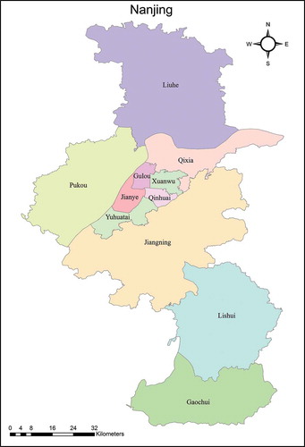
Nanjing is the capital of Jiangsu province in Eastern China. With a total land area of 742.85 km², it is located in the lower Yangtze River drainage basin and the Yangtze River Delta economic zone. In 2010, the urban area had an estimated population of approximately 8,004,680 people. Since February 2013, Nanjing has divided into 11 districts: Gulou, Xuanwu, Jianye, Qinhuai, Yuhuatai, Pukou, Liuhe, Qixia, Jiangning, Lishui, and Gaochun (Figure 1). Previously, Xiaguan and Baixia were separately incorporated into Gulou and Qinhuai. Therefore, the corresponding statistical data from Xiaguan and Baixia (such as population) were merged into that of Gulou and Qinhuai, respectively. Nanjing also boasts an efficient public transportation network, which consists mainly of bus, taxi, and metro systems.

Figure 1. Study area: Nanjing, China has 11 districts with approximately 6500 taxis in daily operation. For full color versions of the figures in this paper, please see the online version.

2.2. Floating Car Data

The FCD was collected from 6445 taxis in Nanjing from 22 February 2010 to 7 March 2010. 22 February and 1 March fall on Monday, and 28 February and 7 March are Sundays. There were 259,421,451 records in total, containing the following attributes: ID, VehicleID, GPSTime, GPSLongtitude, GPSLatitude, GPSSpeed, GPSDirection, and PassengerState. The ID and VehicleID fields are unique identifiers for the FCD records and the taxis, respectively. GPSTime contains an accurate date and time for each record. GPSLongtitude and GPSLatitude separately record the longitude and latitude of the taxi. Speed represents the speed of the taxi at the given time. GPSDirection is a horizontal angle measured clockwise from a north-facing baseline. PassengerState is a Boolean variable that denotes whether the taxi is carrying passengers and has a value of 0 when no passengers are in the taxi and 1 when the taxi is occupied. The average sampling time interval for the FCD is 20–60 s.

3. Methods

In this section, the methods are described. Firstly, passenger pickup and drop-off locations are extracted from FCD and the external passenger pickup and drop-off locations are excluded by spatial filtering. Secondly, Thiessen polygons are introduced to partition the study area. Thirdly, Moran’s I is used to measure spatial autocorrelation. Fourthly, hot spot analysis is used to examine the spatial patterns of pickup and drop-off locations and determine whether they are statistically clustered, dispersed, or random.

3.1. Data preprocessing

3.1.1. Extraction of passenger pickup and drop-off locations

Passenger pickup and drop-off locations can be obtained based on a change in passenger state. When the previous passenger state is 0 and the current passenger state is 1, the current sample point denotes a passenger pickup location. Extracting the passenger pickup and drop-off locations involves three steps: classification, sorting, and searching.

In Step 1 (classification), sample points are classified based on their VehicleID. Sample points with the same VehicleID are assigned to the same group.

In Step 2 (sorting), sample points in the same group are arranged in ascending order according to their GPSTime. In this way, the taxi’s trajectories can be acquired in time sequence.

In Step 3 (searching), sample points in the same group are visited individually. If the previous sample point passenger state is 0 and the current sample point passenger state is 1, the current point is assumed to be a pickup location (see the left side of Figure 2). Similarly, if the previous sample point passenger state is 1 and the current sample point passenger state is 0, the current point is assumed to be a drop-off location (see the right side of Figure 2). A total of 3,225,405 pickup locations and 3,223,506 drop-off locations were extracted.

Figure 2. Extraction of passenger pickup locations and drop-off locations from FCD.

3.1.2. Spatial filtering of passenger pickup and drop-off locations

Although most passenger pickup and drop-off locations occurred within the study area, there were also some pickup and drop-off points that occurred outside the study area. These external passenger pickup and drop-off locations were excluded by spatial filtering, which includes two steps: construction of spatial points and spatial filtering of the points.

In Step 1, the spatial points are constructed. Spatial points contain both geometry features and attribute features. The geometry feature is based on the longitude and latitude of pickup and drop-off locations, while other information from the pickup and drop-off locations are taken as the attribution features.

In Step 2, the spatial points are extracted by clip analysis. Here, the spatial points are the input features and the boundary of the study area is used as the clip feature. Then, spatial clip analysis is executed, and the points that are inside of the study area are retained.

A total of 31,307 pickup locations and 32,491 drop-off locations outside the study area were excluded. Finally, 3,194,098 pickup locations and 3,191,015 drop-off locations were retained. The excluded pickup and drop-off locations comprised only 0.98% and 1.02% of the total pickup and drop-off locations, respectively.

3.2. Spatial partition based on Thiessen polygons

To study the spatial distribution of passenger pickup and drop-off locations, a method for spatial partition of the study area had to be investigated. Because vehicles are driven on the road network, using a regular grid spatial partition method or a partitioning method based on administrative districts would not be ideal. Thiessen polygons are introduced to partition the study area in this research.

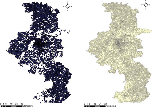
Road nodes (see the left side of Figure 3) are regarded as point input features that can be used to apportion road node coverage into Thiessen polygons (on the right of Figure 3). Each polygon has a unique property that all locations within the polygon are closer to the polygon’s point than to the point of any other polygon. Consequently, each pickup and drop-off location can be assigned to a polygon and the number of such points in each polygon can be obtained. Further information can be investigated based on the Thiessen polygons. A total of 12,558 road nodes and 12,558 Thiessen polygons, respectively, were obtained as shown Figure 3.

Figure 3. Road nodes and their Thiessen polygons of Nanjing. For full color versions of the figures in this paper, please see the online version.

3.3. Spatial autocorrelation of spatial distribution of pickup and drop-off locations

Global spatial statistics look for an overall pattern between proximity and the similarity of regions. These statistics provide a single value that describes the spatial autocorrelation of the dataset as a whole. Moran’s I is a measure widely used in the fields of geography and GIS. Moran’s I is used to measure spatial autocorrelation in this study. A global Moran’s I statistic (Getis and Ord 1992; Ord and Getis 1995) can be estimated for an entire study region and is defined as follows:

(1) $I=\frac{n}{\sum _{i=1}^n\sum _{j=1}^n{w}_{i,j}}\frac{\sum _{i=1}^n\sum _{j=1}^n{w}_{i,j}(x_i-\bar{X})(x_j-\bar{X})}{\sum _{i=1}^n{(x_i-\bar{X})}^2},$(1)

where $n$ is the number of spatial units indexed by $i$ and $j$; $X$ is the variable of interest; $\bar{X}$ is the mean of $X$; and ${w_i}_j$ is an element of a matrix of spatial weights and is the number of points in a Thiessen polygon in this research.

The values of Moran’s I range from −1 to 1. Negative values indicate negative spatial autocorrelation and positive values indicate positive spatial autocorrelation. A zero value indicates a random spatial pattern. Z-score and p-value are usually calculated to indicate whether or not you can reject the null hypothesis.

The z-score indicates the statistical significance given the number of features in the dataset. The z-score can be mathematically represented as follows:

(2) $Z=\frac{1-E(I)}{\sqrt{V(I)}},$(2)

where

(3) $E(I)=-1/(n-1),\mathrm{a}\mathrm{n}\mathrm{d},$(3)

(4) $V(I)=E[I^2]-E[I{]}^2.$(4)

When the absolute value of the z-score is large enough that it falls outside the desired confidence level, the null hypothesis can be rejected. A z-score greater than 2.58 or less than −2.58 indicates that there is less than 1% likelihood that this clustered pattern could be the result of random choice (Mitchell 2005).

The p-value is a probability. If the p-value is very small, it means it is very unlikely that the observed spatial pattern is the result of random processes, so the null hypothesis can be rejected. A p-value less than 0.01 indicates that there is less than 1% likelihood that this clustered pattern could be the result of random choice (Mitchell 2005).

3.4. Hot spot analysis of spatial distribution of pickup and drop-off locations

Local spatial statistics which study local pattern of spatial data are used to measure and test for clustering around a specified geographic location. Hot spot analysis identifies statistically significant spatial clusters with high values (hot spots) and low values (cold spots). Because hot spot areas are statistically significant, the end visualization is less subjective. Therefore, hot spot analysis is used to examine the spatial patterns of pickup and drop-off locations and determine whether they are statistically clustered, dispersed, or random.

A hot spot is represented by an area with a statistically large number of points surrounded by other areas that also contain large numbers of such points. The Getis–Ord (Gi*) statistic for each feature in a dataset are executed. The Getis–Ord local statistic (Getis and Ord 1992; Ord and Getis 1995) is given as:

(5) $G_i^{\ast }=\frac{\sum _{j=1}^n{w}_{i,j}{x}_j-\bar{X}\sum _{j=1}^n{w}_{i,j}}{S\sqrt{\frac{\left[n\sum _{j=1}^n{w}_{i,j}^2-{\left(\sum _{j=1}^n{w}_{i,j}\right)}^2\right]}{n-1}}},$(5)

where $x_j$ is the attribute value for feature j, $w_{i,j}$ is the spatial weight between feature i and j, n is equal to the total number of features and

(6) $\bar{X}=\frac{\sum _{j=1}^n{x}_j}{n},\mathrm{a}\mathrm{n}\mathrm{d}$(6)

(7) $S=\sqrt{\frac{\sum _{j=1}^n{x}_j^2}{n}-{\left(\bar{X}\right)}^2}.$(7)

4. Results

In this section, the results are shown. Firstly, the number of pickup locations and drop-off locations over time is showed. Secondly, spatial distribution of the pickup and drop-off locations is showed. Lastly, spatial and temporal distributions of pickup locations during some typical periods are showed.

4.1. Temporal patterns of passenger pickup and drop-off locations

After extracting all the passenger pickup and drop-off locations, the statistics of the occurrences of pickup and drop-off locations during each day and each hour can be obtained easily. The number of both pickup and drop-off locations during each day and each hour are plotted in Figure 4.

Figure 4. The number of pickup locations and drop-off locations over time. (a) The number of pickup locations and drop-off locations each day; (b) The number of pickup locations and drop-off locations each hour. For full color versions of the figures in this paper, please see the online version.

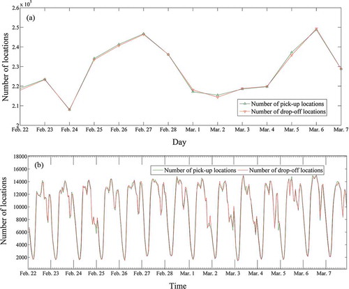
From a day-scale perspective, the following conclusions can be drawn. The number of pickup locations and the number of drop-off locations are approximately equal every day. The pattern with two distinct peaks that appear on Saturday (27 February and 6 March) can be seen in Figure 4(a). Moreover, the numbers of points on Fridays (26 February and 5 March), Saturdays (27 February and 6 March), and Sundays (28 February and 7 March) are larger than that on other days. As is common knowledge, urban residents usually start their weekend on Friday night, and it extends through Sunday. The number of people who travel by taxi on weekends is larger than the number who travel by taxis on weekdays.

From the hour-scale perspective, some interesting temporal patterns can also be discovered (Figure 4(b)). A similar pattern appears every day and the temporal distribution of the pickup and drop-off locations represents a strong daily rhythm. The number of pickup locations and the number of drop-off locations show similar characteristics. The plots indicate two valleys: 4:00–6:00 and 19:00–21:00. There is an obvious period of increase from 7:00 to 10:00 and an obvious decline from 23:00 to 5:00. Both the pickup locations and drop-off locations exist in great numbers from 10:00 to 18:00. During the day (from 6:00 to 21:00), there is no significant difference between the number of pickup and drop-off locations on weekends and weekdays. However, at night (from 21:00 to 6:00), the number of pickup locations or drop-off locations on weekends is larger than that on weekdays.

4.2. Spatial patterns of passenger pickup and drop-off locations

Based on the number of pickup and drop-off locations in Thiessen polygons, the spatial distribution and cluster characteristics of the number of people traveling by taxi are studied.

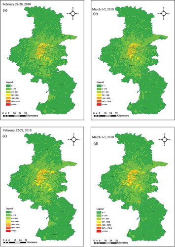
Both the spatial distribution of pickup locations (Figure 5(a,b)) and the spatial distribution of drop-off locations (Figure 5(c,d)) are shown. A rating scale is used to define the interval in Figure 5(a–d). Although the time periods are different, the spatial distribution of pickup locations and drop-off locations has similar spatial patterns. The districts of Nanjing can be divided into three groups according to the spatial distribution of pickup locations and drop-off locations. Xuanwu, Qinhuai, Yuhuatai, Gulou, Jianye are in the first group in the downtown area of Nanjing; large numbers of points are concentrated within these districts. Pukou, Liuhe, Qixia, and Jiangning are in the second group in the Nanjing suburbs; the number of points in these districts is smaller than in those of the first group. Lishui and Gaochun, which are in the outer suburbs of Nanjing, compose the third group; only small numbers of points are located in these districts. Obviously, the number of pickup and drop-off locations gradually diminishes from the first to the third group. However, the small region with the orange color in Figure 5(a–d) that is far away from the downtown area is the Lukou International Airport.

Figure 5. Spatial distribution of the pickup and drop-off locations. (a) Spatial distribution of the pickup locations from 22 February to 28 February; (b) Spatial distribution of the pickup locations from 1 March to 7 March; (c) Spatial distribution of the drop-off locations from 22 February to 28 February; (b) Spatial distribution of the drop-off locations from 1 March to 7 March. For full color versions of the figures in this paper, please see the online version.

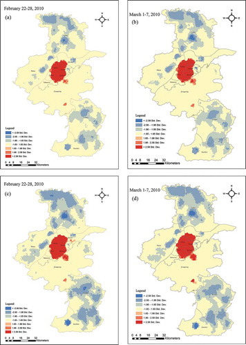
Both hot spots and cold spots of the pickup locations (Figure 6(a,b)) and the drop-off locations (Figure 6(c,d)) were plotted. In Figure 6, standard deviation (std. dev.) is used to quantify the amount of points in the region. The hot and cold spots of pickup locations and of drop-off locations showed similar spatial patterns. Both the hot spots of the pickup locations and those of the drop-off locations are concentrated in the downtown area and at the Lukou International Airport, while most of the cold spots are located in Pukou, Liuhe, Lishui, and Gaochun. A small number of cold spots appear in Xuanwu, Qixia, and Jiangning.

Figure 6. Hot spot analysis of the pickup and drop-off locations. (a) Hot spot analysis of pickup locations from 22 February to 28 February; (b) Hot spot analysis of pickup locations from 1 March to 7 March; (c) Hot spot analysis of drop-off locations from 22 February to 28 February; (d) Hot spot analysis of drop-off locations from 1 March to 7 March. For full color versions of the figures in this paper, please see the online version.

4.3. Spatiotemporal patterns of passenger pickup and drop-off locations

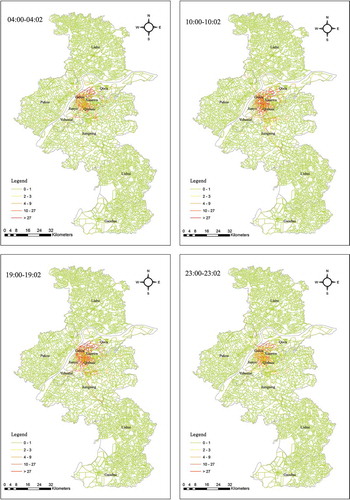
To study spatiotemporal patterns, maps at day and hour scales showing pickup and drop-off locations from 22 February to 7 March were made. At a day scale, the maps present similar spatial patterns. The spatial distribution of pickup and drop-off locations at an hourly scale exhibits similar spatial patterns at corresponding hours on different days. However, the maps present different spatial distribution characteristics for different hours within the same day. Some typical time periods of the spatial distribution of pickup and drop-off locations on 3 March are shown in Figure 7. Generally, the number of pickup and drop-off locations in each region changes over time. In addition, the number of pickup and drop-off locations during the day (from 10:00 to 11:00) is higher than that in other hours (04:00–05:00, 19:00–20:00, and 23:00–24:00). Moreover, the number of pickup and drop-off locations within the center of the city or nearby is larger than in the suburbs. Furthermore, the number of pickup and drop-off locations at the center of the city or nearby changes more dramatically than pickup and drop-off locations in the suburbs.

Figure 7. Spatial and temporal distributions of pickup and drop-off locations on 3 March during some typical periods. (a) Spatial and temporal distributions of pickup locations; (b) Spatial and temporal distributions of drop-off locations. For full color versions of the figures in this paper, please see the online version.

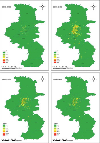
Figure 7. (Continued)

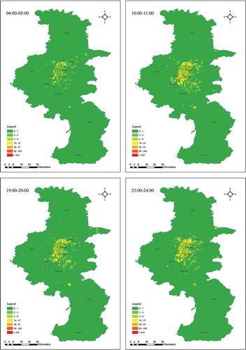
To study spatiotemporal patterns, taxi-passing map were made. Some typical time periods of the spatial distribution of taxi on 3 March are shown in Figure 8. In addition to the conclusions from Figure 7, we can also conclude that people more likely taking taxi at the main street in contrast with alleyway, same with the taxi driver.

Figure 8. Taxi-passing map on 3 March during some typical periods. For full color versions of the figures in this paper, please see the online version.

Moran’s I indices were calculated to express the spatial autocorrelation of regions and the resulting values are plotted in Figure 9. The following conclusions can be derived from Figure 9(a). Both the Moran’s I indices of the spatial distribution of pickup locations and that of drop-off locations are larger than zero, indicating positive spatial autocorrelation. Each day exhibits one valley from 5:00 to 7:00, indicating that the spatial distribution of pickup locations and drop-off locations is very discrete during this period. There is one obvious rising period from 7:00 to 10:00 and one decreasing period from 1:00 to 5:00. In contrast with Figure 4(b) and Figure 9(a), Moran’s I index is consistent with the number of pickup or drop-off locations to some extent. One peak appears between 22:00 and 23:00 every day (which means that the locations of people’s activities are more concentrated at night). On the hour scale, the minimum z-score value is larger than 60 and the maximum p-value is less than 0.01, indicating a less than 1% likelihood that this clustered pattern could be the result of random choice.

Figure 9. Changes in the Moran’s I index over time. (a) Moran’s I index of spatial distribution of pickup and drop-off locations changes by hour; (b) Comparative analysis of minimum and maximum Moran’s I index values on hourly and daily scales. For full color versions of the figures in this paper, please see the online version.

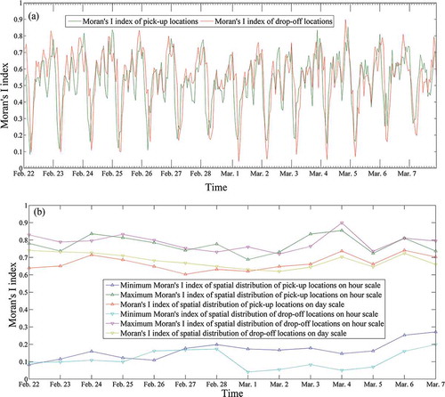
By contrasting the Moran’s I index at day and hour scales (Figure 9(b)), the following conclusions can be reached. Moran’s I index at the day scale is larger than the minimum value at the hour scale and smaller than the maximum value of the hour scale every day. The number of points for an entire day is certainly greater than the amount of points at any given hour. However, Moran’s I index for a whole day is smaller than that for some hours. Therefore, Moran’s I index is not completely consistent with the number of points. Moran’s I index is affected by both the number of points and their spatial distribution.

5. Discussion

In this section, the driving forces that affect the spatial distribution of pickup locations and drop-off locations are analyzed. In this study, regression analyses for the relationships between the density of pickup/drop-off locations and population density, transportation density and per capita disposable income were modeled. As mentioned in Section 3, Xiaguan and Baixia were previously separately incorporated into Gulou and Qinhuai, respectively. Therefore, the population size of Gulou and Qinhuai is the sums of the population size of previous districts, and the road length of Gulou and Qinhuai is the sums of the road length of previous districts. Because the per capita disposable income is the amount of discretionary income an individual, the per capita disposable income of Gulou and Qinhuai are weight sums of the per capita disposable income of previous districts.

R² is used to measure the strength of the prediction relationship between the explanatory and dependent variables. An R² value closer to 1 indicates a strong prediction relationship. F-tests are used to test the null hypothesis that there is no linear relationship between the explanatory and the dependent variables. When the significance level for the F-test is low, a linear relationship exists. P-values are widely used in statistical hypothesis testing. When the p-value is less than or equal to a chosen significance level, the null hypothesis can be rejected. The R², F-test, and p-value measures are introduced to test the regression models.

As a dependent variable, the density of pickup locations and that of drop-off locations in each district is defined as

(8) $PtDensity=\frac{PtNum}{Area},$(8)

where $PtNum$ is the number of pickup or drop-off locations, $Area$ is the area of the district, and $PtDensity$ is the point density. The unit is the number of points per square kilometer.

As an explanatory variable, population density is a measurement of population per unit area defined as follows:

(9) $PopDensity=\frac{PopNum}{Area},$(9)

where $PopNum$ is the population size, $Area$ is the area of the district, and $PopDensity$ is the population density. The unit is the population size per square kilometer.

As an explanatory variable, road density is a measurement of road length per unit area:

(10) $RoadDensity=\frac{RoadLen}{Area},$(10)

where $RoadLen$ is the total road length of the district and $RoadDensity$ is the road density. The unit is meters per square kilometer.

As an explanatory variable, per capita disposable income is the amount of discretionary income an individual that has to purchase goods and services. The per capita disposable income of Gulou and Qinhuai is defined as follows:

(11) $PCDI=\frac{\sum _{i=1}^n{w}_i\times PCD{I}_i}{\sum _{i=1}^n{w}_i},\mathrm{a}\mathrm{n}\mathrm{d}$(11)

(12) $w_i=\frac{PopNu{m}_i}{\sum _{i=1}^{n}PopNu{m}_i},$(12)

where $PCDI$ is the per capita disposable income of the district, $PCD{I}_i$ is the per capita disposable income of the previous i-th district, and $w_i$ is the weight of the previous i-th district as determined by the population size.

Four multiple regression models for modeling the relationships between the density of pickup/drop-off locations and population density, transportation density and per capita disposable income are built. The multiple regression models are given in Formulas 13–16.

(13) $y_1=-2769.2336+0.2699x_1+0.8515x_2+0.0395x_3$(13)

(14) $y_2=-3042.7558+0.2790x_1+0.6648x_2+0.0639x_3$(14)

(15) $y_3=-2511.6466+0.2832x_1+0.7286x_2+0.0378x_3$(15)

(16) $y_4=-3208.8014+0.2865x_1+0.5736x_2+0.0765x_3,$(16)

where $y_1$, $y_2$, $y_3$, and $y_4$ denote the density of the pickup locations from 22 February to 28 February, the density of the drop-off locations from 22 February to 28 February, the density of the pickup locations from 1 March to 7 March, and the density of the drop-off locations from 1 March to 7 March, respectively; $x_1$, $x_2$, and $x_3$ are the population density, transportation density, and per capita disposable income, respectively.

The values of R² obtained from Formulas 13–16 are 0.9893, 0.9949, 0.9945, and 0.9963, respectively. All the R² values are close to 1, indicating strong prediction relationships.

The values of the F-tests from Formulas 13–16 are 8.3893E-08, 2.2103E-08, 2.8354E-08, and 6.9995E-09, respectively. These are all close to 0, indicating linear relationships between the explanatory and dependent variables.

The p-values of $x_1$, $x_2$, and $x_3$ in Formula 13 are 3.5340E-05, 0.0028, and 0.6578, respectively; while in Formula 14, they are 6.1423E-06, 0.0030, and 0.3778, respectively. The p-values of $x_1$, $x_2$, and $x_3$ in Formula 15 are 8.3306E-06, 0.0025, and 0.6166, respectively; while in Formula 16, they are 1.5600E-06, 0.0026, and 0.2208, respectively. All the p-values for $x_1$ and $x_2$ from Formula 13 to Formula 16 are below the chosen significance level (5%); consequently, the null hypothesis is rejected. However, all the p-values for $x_3$ are higher than the chosen significance level (5%); consequently, the null hypothesis is not rejected. Therefore, population density and transportation density are consistent with the regression models, but per capita disposable income is not consistent with the regression models.

6. Conclusions

This study used a large volume of taxi-based FCD to uncover people’s spatiotemporal behavior patterns. The temporal distribution of taxi pickup and drop-off locations exhibits a strong daily rhythm, and urban residents take more taxis during the day than at night. The overall spatial pattern shows that the number of pickup locations or drop-off locations gradually diminishes from the downtown area to the outer suburbs. Hot spots of the pickup locations and those of the drop-off locations are concentrated in downtown Nanjing and at the Lukou International Airport. The spatial distribution of pickup locations or drop-off locations exhibits huge differences over time. The relationships between the density of pickup/drop-off locations and population density, transportation density and per capita disposable income were modeled, and the results show that population density and transportation density are consistent with the regression models, but per capita disposable income is not consistent with the regression models.

The major novel contribution of this paper lies in discovering people’s spatiotemporal behavior patterns from a large volume of taxi-based FCD. The first characteristic of the study is that many geospatial statistical methods are used to analyze FCD. Future conclusion can be drawn that geospatial statistical methods can be used to analyze other location-based data. This research may broaden the application of GIS. The second characteristic of the study is that a large volume of FCD is used. FCD is high volume and high volume is an important characteristic of big data. The research may have certain reference significance for the study of big data.

Although this study analyzed 2 weeks of FCD data, the FCD for holidays was often missing; therefore, the spatial and temporal patterns of holidays were not considered. This study proposed a method for extracting passenger pickup and drop-off locations based on changes of passenger state. The accurate pickup or drop-off locations are located between such two consecutive points. Because the sampling time interval for the FCD was only 20–60 s, the positional error of pickup or drop-off locations was ignored in this research. Because it is impossible to obtain an accurate estimate of the number of people in each Voronoi region, population density and per capita disposable income are based on statistics for the district. Road density is also district based to maintain consistency with population density and per capita disposable income.

There are many rivers, lakes, and mountains in Nanjing, and the impact of these features are not considered in this study when building Thiessen polygon. The impact of these features will be considered in the future. Taxis are only one important way to travel, but only taxi-based FCD were explored in this research. If data for all types of travel could be obtained, the conclusions would be more comprehensive. There is no doubt that discovering spatiotemporal behavior patterns based on multisource data will contribute to many other studies in the future, such as comprehensive (including human and natural factors) Digital Earth (e.g., Craglia et al. 2008; Guo et al. 2014) and Virtual Geographic Environments (e.g., Lin, Chen, and Lu 2013; Lin et al. 2013, 2015; Chen et al. 2015; Zhang et al. 2016).

Acknowledgments

We appreciate the detailed suggestions and constructive comments from the editor and the anonymous reviewers. This research was jointly supported by the National Natural Science Foundation of China (No. 41301417, No. 41622108), PAPD (164320H116), the Chongqing Natural Science Foundation (No. cstc2014jcyjA20017), and the Fundamental Research Funds for the Central Universities (No. XDJK2015B022).

Disclosure statement

No potential conflict of interest was reported by the authors.

Additional information

Funding

This research was jointly supported by the National Natural Science Foundation of China (numbers 41301417, 41622108), PAPD (164320H116), the Chongqing Natural Science Foundation (No. cstc2014jcyjA20017), and the Fundamental Research Funds for the Central Universities (numebr XDJK2015B022).

References

- Asakura, Y., and T. Iryo. 2007. “Analysis of Tourist Behaviour Based on the Tracking Data Collected Using a Mobile Communication Instrument.” Transportation Research Part A Policy & Practice 41 (7): 684–690. doi:10.1016/j.tra.2006.07.003.
- Bar-Gera, H. 2007. “Evaluation of A Cellular Phone-Based System for Measurements of Traffic Speeds and Travel Times: A Case Study from Israel.” Transportation Research Part C Emerging Technologies 15 (6): 380–391. doi:10.1016/j.trc.2007.06.003.
- Bierlaire, M., J. Chen, and J. Newman. 2013. “A Probabilistic Map Matching Method for Smartphone GPS Data.” Transportation Research Part C Emerging Technologies 26 (1): 78–98. doi:10.1016/j.trc.2012.08.001.
- Castro, P. S., D. Zhang, and S. Li. 2012. “Urban Traffic Modelling and Prediction Using Large Scale Taxi GPS Traces.” In Pervasive Computing, 57–72. Berlin: Springer-Verlag. doi:10.1007/978-3-642-31205-2_4.
- Chang, H. W., Y. C. Tai, and Y. J. Hsu. 2010. “Context-Aware Taxi Demand Hotspots Prediction.” International Journal of Business Intelligence & Data Mining 5 (1): 3–18. doi:10.1504/IJBIDM.2010.030296.
- Chen, M., H. Lin, O. Kolditz, and C. Chen. 2015. “Developing Dynamic Virtual Geographic Environments (VGEs) for Geographic Research.” Environmental Earth Sciences 74: 6975–6980. doi:10.1007/s12665-015-4761-4.
- Craglia, M., M. F. Goodchild, A. Annoni, G. Camara, M. Gould, W. Kuhn, D. Mark, et al. 2008. “Next-Generation Digital Earth—A Position Paper from the Vespucci Initiative for the Advancement of Geographic Information Science.” International Journal of Spatial Data Infrastructures Research 3: 146–167. doi:10.2902/1725-0463.2008.03.art9.
- Ehmke, J. F., S. Meisel, and D. C. Mattfeld. 2012. “Floating Car Based Travel Times for City Logistics.” Transportation Research Part C: Emerging Technologies 21 (1): 338–352. doi:10.1016/j.trc.2011.11.004.
- Fontaine, M., B. Smith, and M. Fontaine. 2005. “Probe-Based Traffic Monitoring Systems with Wireless Location Technology: An Investigation of the Relationship between Systems Design and Effectiveness.” Transportation Research Record Journal of the Transportation Research Board 1: 2–11. doi:10.3141/1925-01.
- Gao, S., Y. Wang, Y. Gao, and Y. Liu. 2013. “Understanding Urban Traffic-Flow Characteristics: A Rethinking of Betweenness Centrality.” Environment & Planning B Planning & Design 40 (1): 135–153. doi:10.1068/b38141.
- Getis, A., and J. K. Ord. 1992. “The Analysis of Spatial Association by Use of Distance Statistics.” Geographical Analysis 24 (3): 189–206. doi:10.1111/j.1538-4632.1992.tb00261.x.
- Guo, D., X. Zhu, H. Jin, P. Gao, and C. Andris. 2012. “Discovering Spatial Patterns in Origin-Destination Mobility Data.” Transactions in GIS 16 (3): 411–429. doi:10.1111/j.1467-9671.2012.01344.x.
- Guo, H. D., L. Z. Wang, F. Chen, and D. Liang. 2014. “Scientific Big Data and Digital Earth.” Chinese Science Bulletin 59 (35): 5066–5073. doi:10.1007/s11434-014-0645-3.
- Kang, H., and D. M. Scott. 2008. “An Integrated Spatio-Temporal GIS Toolkit for Exploring Intra-Household Interactions.” Transportation 35 (2): 253–268. doi:10.1007/s11116-007-9146-4.
- Kong, X., Z. Xu, G. Shen, J. Wang, Q. Yang, and B. Zhang. 2016. “Urban Traffic Congestion Estimation and Prediction Based on Floating Car Trajectory Data.” Future Generation Computer Systems 61: 97–107. doi:10.1016/j.future.2015.11.013.
- Lee, J., I. Shin, and G. L. Park. 2008. “Analysis of the Passenger Pick-Up Pattern for Taxi Location Recommendation.” In Proceedings of the International Conference on Networked Computing and Advanced Information Management, 199–204. Gyeongju. doi:10.1109/NCM.2008.24.
- Li, Q., Z. Zeng, T. Zhang, J. Li, and Z. Wu. 2011. “Path-Finding Through Flexible Hierarchical Road Networks: An Experiential Approach Using Taxi Trajectory Data.” International Journal of Applied Earth Observation & Geoinformation 13 (1): 110–119. doi:10.1016/j.jag.2010.07.003.
- Li, Q., T. Zhang, H. Wang, and Z. Zeng. 2011. “Dynamic Accessibility Mapping Using Floating Car Data: A Network-Constrained Density Estimation Approach.” Journal of Transport Geography 19 (3): 379–393. doi:10.1016/j.jtrangeo.2010.07.003.
- Lin, H., M. Batty, S. E. Jørgensen, B. J. Fu, M. Konecny, A. Voinov, P. Torrens, et al. 2015. “Virtual Environments Begin to Embrace Process-Based Geographic Analysis.” Transactions in GIS 19 (4): 493–498. doi:10.1111/tgis.12167.
- Lin, H., M. Chen, and G. N. Lu. 2013. “Virtual Geographic Environment: A Workspace for Computer-Aided Geographic Experiments.” Annals of the Association of American Geographers 103 (3): 465–482. doi:10.1080/00045608.2012.689234.
- Lin, H., M. Chen, G. N. Lu, Q. Zhu, J. H. Gong, X. You, Y. N. Wen, B. L. Xu, and M. Y. Hu. 2013. “Virtual Geographic Environments (VGES): A New Generation of Geographic Analysis Tool.” Earth-Science Reviews 126: 74–84. doi:10.1016/j.earscirev.2013.08.001.
- Liu, L., C. Andris, and C. Ratti. 2010. “Uncovering Cabdrivers’ Behavior Patterns from Their Digital Traces.” Computers, Environment and Urban Systems 34 (6): 541–548. doi:10.1016/j.compenvurbsys.2010.07.004.
- Liu, X., and Y. Ban. 2013. “Uncovering Spatio-Temporal Cluster Patterns Using Massive Floating Car Data.” ISPRS International Journal of Geo-Information 2 (1): 1–15. doi:10.3390/ijgi2020371.
- Liu, X., L. Gong, Y. Gong, and Y. Liu. 2015. “Revealing Travel Patterns and City Structure with Taxi Trip Data.” Journal of Transport Geography 43: 78–90. doi:10.1016/j.jcrysgro.2015.01.022.
- Liu, X., F. B. Zhan, and T. Ai. 2010. “Road Selection Based on Voronoi Diagrams and “Strokes” in Map Generalization.” International Journal of Applied Earth Observation and Geoinformation 12: 194–202. doi:10.1016/j.jag.2009.10.009.
- Liu, Y., F. Wang, Y. Xiao, and S. Gao. 2012. “Urban Land Uses and Traffic ‘Source-Sink Areas’: Evidence from GPS-Enabled Taxi Data in Shanghai.” Landscape and Urban Planning 106 (1): 73–87. doi:10.1016/j.landurbplan.2012.02.012.
- Long, T. T., and S. V. C. Somenahalli. 2011. “Using GIS to Identify Pedestrian-Vehicle Crash Hot Spots and Unsafe Bus Stops.” Journal of Public Transportation 14 (1): 99–114. doi:10.5038/2375-0901.14.1.6.
- Lu, M., Z. Wang, J. Liang, and X. Yuan. 2015. “OD-Wheel: Visual Design to Explore OD Patterns of a Central Region.” 2015 IEEE Pacific Visualization Symposium (PacificVis), Hangzhou, China, 87–91. doi:10.1109/PACIFICVIS.2015.7156361.
- Mao, F., M. Ji, and T. Liu. 2016. “Mining Spatiotemporal Patterns of Urban Dwellers from Taxi Trajectory Data.” Frontiers of Earth Science 10 (2): 205–221. doi:10.1007/s11707-015-0525-4.
- Mitchell, A. 2005. The ESRI Guide to GIS Analysis. Vol. 2. RedLands, CA: ESRI Press.
- Mu, C., and X. Zhao. 2011. “Dynamic Passenger OD Distribution and System Performance of Taxi Operation System.” International Journal of Information Engineering and Electronic Business 3 (2): 56–63. doi:10.5815/ijieeb.2011.02.08.
- Ord, J. K., and A. Getis. 1995. “Local Spatial Autocorrelation Statistics: Distributional Issues and an Application.” Geographical Analysis 27 (4): 286–306. doi:10.1111/j.1538-4632.1995.tb00912.x.
- Park, S. J. 2012. “Measuring Public Library Accessibility: A Case Study Using GIS.” Library & Information Science Research 34 (1): 13–21. doi:10.1016/j.lisr.2011.07.007.
- Patil, P., and A. Gokhale. 2013. “Voronoi-Based Placement of Road-Side Units to Improve Dynamic Resource Management in Vehicular Ad Hoc Networks.” 2013 International Conference on Collaboration Technologies and Systems (CTS), San Diego, CA, 389–396. doi:10.1109/CTS.2013.6567260.
- Qian, X., and S. Ukkusuri. 2015. “Spatial Variation of the Urban Taxi Ridership Using GPS Data.” Applied Geography 59: 31–42. doi:10.1016/j.apgeog.2015.02.011.
- Sang, W. B., and K. Y. Chwa. 2004. “Voronoi Diagrams with a Transportation Network on the Euclidean Plane.” International Journal of Computational Geometry & Applications 16 (2n03): 101–112. doi:10.1007/978-3-540-30551-4_11.
- Schwieger, V., K. Ramm, R. Czommer, and W. Möhlenbrink. 2007. “Mobile Phone Positioning for Traffic State Acquisition.” Journal of Applied Geodesy, no. 1: 125–135. doi:10.1080/17489720701779651.
- Simroth, A., and H. Zahle. 2011. “Travel Time Prediction Using Floating Car Data Applied to Logistics Planning.” IEEE Transactions on Intelligent Transportation Systems 12 (1): 243–253. doi:10.1109/TITS.2010.2090521.
- Su, J. G., M. Jerrett, B. Beckerman, M. Wilhelm, J. K. Ghosh, and B. Ritz. 2009. “Predicting Traffic-Related Air Pollution in Los Angeles Using a Distance Decay Regression Selection Strategy.” Environmental Research 109 (6): 657–670. doi:10.1016/j.envres.2009.06.001.
- Tao, S., J. Corcoran, I. Mateo-Babiano, and D. Rohde. 2014. “Exploring Bus Rapid Transit Passenger Travel Behaviour Using Big Data.” Applied Geography 53: 90–104. doi:10.1016/j.apgeog.2014.06.008.
- Tobler, W. 1970. “A Computer Movie Simulating Urban Growth in the Detroit Region.” Economic Geography 46 (2): 234–240. doi:10.2307/143141.
- Uno, N., F. Kurauchi, H. Tamura, and I. Yasunori. 2009. “Using Bus Probe Data for Analysis of Travel Time Variability.” Journal of Intelligent Transportation Systems 13 (1): 2–15. doi:10.1080/15472450802644439.
- Wang, J., M. Kwan, and L. Ma. 2014. “Delimiting Service Area Using Adaptive Crystal-Growth Voronoi Diagrams Based on Weighted Planes: A Case Study in Haizhu District of Guangzhou in China.” Applied Geography 50: 108–119. doi:10.1016/j.apgeog.2014.03.001.
- Wang, S., L. Sun, J. Rong, and Z. Yang. 2014. “Transit Traffic Analysis Zone Delineating Method Based on Thiessen Polygon.” Sustainability 6 (4): 1821–1832. doi:10.3390/su6041821.
- Yamada, I., and J. C. Thill. 2007. “Local Indicators of Network-Constrained Clusters in Spatial Point Patterns.” Geographical Analysis 39 (39): 268–292. doi:10.1111/j.1538-4632.2007.00704.x.
- Yang, Z. Z., L. Wang, and G. Chen. 2007. “Method of Traffic Analysis Zone Partition for Traffic Impact Assessment.” Journal of Highway & Transportation Research & Development 2 (2): 80–83. doi:10.1061/JHTRCQ.0000200.
- Yue, Y., Y. Zhuang, Q. Li, and Q. Mao. 2009. “Mining Time-Dependent Attractive Areas and Movement Patterns from Taxi Trajectory Data.” International Conference on Geoinformatics, Fairfax, VA. IEEE, 1–6. doi:10.1109/GEOINFORMATICS.2009.5293469.
- Zhang, C. X., M. Chen, R. R. Li, C. Y. Fang, and H. Lin. 2016. “What’s Going on about Geo-Process Modeling in Virtual Geographic Environments (Vges).” Ecological Modelling 319: 147–154. doi:10.1016/j.ecolmodel.2015.04.023.
- Zhao, J., A. Rahbee, and N. H. M. Wilson. 2007. “Estimating a Rail Passenger Trip Origin-Destination Matrix Using Automatic Data Collection Systems.” Computer-Aided Civil and Infrastructure Engineering 22 (5): 376–387. doi:10.1007/978-3-642-20244-5_48.
- Zhu, B., Q. Huang, L. Guibas, and L. Zhang. 2013. “Urban Population Migration Pattern Mining Based on Taxi Trajectories.” 3rd International Workshop on Mobile Sensing: The Future, Brought to You by Big Sensor Data, Philadelphia.April 8.