Normalizing shadows in multi-temporal aerial frame imagery using relative radiometric adjustments to support near-real-time change detection

Abstract

This study addresses the problem of shadows in multi-temporal imagery, which is a key issue with change detection approaches based on image comparison. We apply image-to-image radiometric normalizations including histogram matching (HM), mean-variance (MV) equalization, linear regression based on pseudo-invariant features (PIF-LR), and radiometric control sets (RCS) representing high- and low-reflectance extrema, for the novel purpose of normalizing brightness of transient shadows in high spatial resolution, bi-temporal, aerial frame image sets. Efficient shadow normalization is integral to remote sensing procedures that support disaster response efforts in a near-real-time fashion, including repeat station image (RSI) capture, wireless data transfer, shadow detection (as precursor to shadow normalization), and change detection based on image differencing and visual interpretation. We apply the normalization techniques to imagery of suburban scenes containing shadowed materials of varied spectral reflectance characteristics, whereby intensity (average of red, green, and blue spectral band values) under fully illuminated conditions is known from counterpart reference images (time-1 versus time-2). We evaluate the normalization results using stratified random pixel samples within transient shadows, considering central tendency and variance of differences in intensity relative to the unnormalized images. Overall, MV equalization yielded superior results in our tests, reducing the radiometric effects of shadowing by more than 85 percent. The HM and PIF-LR approaches showed slightly lower performance than MV, while the RCS approach proved unreliable among scenes and among stratified intensity levels. We qualitatively evaluate a shadow normalization based on MV equalization, describing its utility and limitations when applied in change detection. Application of image-to-image radiometric normalization for brightening shadowed areas in multi-temporal imagery in this study proved efficient and effective to support change detection.

Keywords:

• shadow normalization
• radiometric normalization
• shadow detection
• repeat station imaging
• image processing

Introduction

Accurate and timely information on the type, severity, and spatial extent of damages to civil infrastructure resulting from hazardous events can be critical in emergency response efforts. High spatial resolution, geometrically co-registered aerial imagery acquired before and after such an event is a viable basis for detecting surficial changes efficiently for large areas (Lippitt and Stow 2015). Automated change detection may be complementary to visual image interpretation for applications requiring expedited analysis of large data sets. However, change detections based on image differencing and post-classification comparison are subject to artifacts of geometric misalignment, and of radiometric variations due to shadows and dynamic illumination conditions (Benediktsson and Sveinsson 1997; Wang et al. 1999; Dala Mura et al. 2008; Stow et al. 2016). Improved techniques to reduce such artifacts are needed with the advent of commercial satellite, large-format aerial, and unpiloted aerial imaging systems, which provide imagery of high spatial resolution to support a broadening range of applications (Turner et al. 2014).

Parallax effects which contribute to geometric misalignment in multi-temporal aerial frame imagery can be minimized by camera triggering at nearly identical vertical and horizontal coordinates (Stow, Coulter, and Baer 2003; Coulter, Stow, and Baer 2003; Coulter et al. 2015), an approach termed repeat station imaging (RSI). RSI enables highly accurate image co-registration, thereby improving our capacity to detect damage features, and to distinguish them from dynamic features such as automobiles and shadows.

Shadows that have changed in orientation or extent between imaging times (transient shadows) are especially problematic for change detection, as compared to shadows that appear stationary in multi-temporal imagery (persistent shadows). Spectral-radiometric (SR) changes, associated with differences in illumination (direct versus diffuse) and shadow positions in multi-temporal imagery, provide a basis for classifying transient shadows and distinguishing them from other changed features (Storey et al. 2017). Effects of shadowing include reduction in net radiance, accompanied by increase in relative radiance of shorter visible wavelengths (especially blue) due to diffuse atmospheric illumination (Liu and Yamazaki 2012). Shadow maps of considerable accuracy (83–97 percent) can be derived by applying a versatile, threshold-based classification of pixel-level differences between time-1 and time-2 of an image set, including brightness (intensity) and the blue spectral band normalized by intensity (Storey et al. 2017). Classified shadow features can be precluded from a change detection, yet this results in a loss of image data that may represent important changes within shadows (Dare 2005). In order to extract information from shadowed areas, augmenting digital number (DN) or intensity values to approximate directly-illuminated conditions is generally required (Li, Zhang, and Shen 2014); we refer to this task as shadow normalization. This study addresses shadow normalization from a radiometric and remote sensing perspective, for the purpose of rapid change detection in built environments based on high spatial resolution, aerial frame imagery. Primarily, this study evaluates the novel approach of extracting radiometric information from transient shadows in co-registered multi-temporal image sets as a basis for shadow normalization.

The intensities of pixels that are classified as shadow (we refer to the set of pixels within an image as S), can be augmented based on statistical or histogram data derived from the directly-illuminated (D-I) pixels of the same image (Shu and Freeman 1990; Silva et al. 2017). Potential differences in material composition and reflectance between the S and D-I pixels of a scene, however, cause uncertainty in this type of shadow normalization (cf. Dare 2005). To address this issue, pixels must be classified according to material type using supervised object-based image analysis (OBIA) and radiometrically normalized between S and D-I areas (Guo, Dai, and Hoiem 2011, 2013). Limitations of this approach are that materials in the S area may lack counterparts in the D-I area, while segmentation and classification parameters are highly scene-dependent and potentially time-expensive to identify (Laliberte, Browning, and Rango 2012; Storey et al. 2017). Furthermore, the presence of compound shadow features (which include several adjacent material types with distinct spectral signatures, such as asphalt and concrete) may hinder image matting (or “soft shadow”) and thin-plate operations commonly used in shadow normalization based on OBIA (Li, Zhang, and Shen 2014). Image matting may also obscure fine-scale features such as fracture damages in transportation infrastructure. Pixel-based shadow normalization approaches, which are more computationally efficient than OBIA (cf. Sanin, Sanderson, and Lovell 2012) and that rely on radiometric information over material type classification, appear most suitable for the application of this study.

We use the term overlay to refer to pixel-level comparison of co-registered, multi-temporal imagery, by means of statistical sampling or visual interpretation. Multi-temporal image overlay for the purpose of detecting transient shadows was employed in Storey et al. (2017), though the utility of image overlay for shadow normalization was not evaluated in a substantive manner. Multi-date image fusion (an approach similar to image overlay) was employed to remove cloud shadows in satellite imagery, by substituting S pixels with pixels from a different image in which the corresponding areas are D-I (Wang et al. 1999). Given that features in shadows may change between image acquisitions, data fusion is inherently problematic for shadow normalizations used to support change detection. Nonetheless, radiometric information from transient shadow areas may retain considerable utility as a basis for shadow normalization.

Employing the terminology of classical image-to-image radiometric normalization, we may consider the transient shadow pixel set as a zone (the subject) that exhibits distinct and substantial illumination change from the D-I condition (the reference), affecting spectral radiance of the surfaces therein. A basic way to adjust the intensity distribution of a subject pixel set to approximate a reference pixel set is to equalize their global mean values. Because shadowing compresses dynamic range, a coupled mean-variance adjustment is appropriate (cf. Shu and Freeman 1990; Dare 2005; Liu and Yamazaki 2012):

(1)

where DN_i is the input pixel value, µ_S and µ_DI represent the S and D-I mean values, σ_S and σ_DI represent the S and D-I standard deviation values, and DN_r is the resulting (normalized) pixel value.

The technique of histogram matching may also be useful for normalizing transient shadows in multi-temporal imagery, although it was found to be less effective than mean-variance adjustment for mono-temporal images (Shu and Freeman 1990). Our preparatory work suggests that shadows not only compress dynamic range but also change the shape of probability density functions (histograms) associated with transient shadows, in the absence of physical changes. Histogram matching could be useful to ameliorate this problem, though it appears untested in relevant literature as a basis for normalizing transient shadows based on image overlay.

A key issue in normalizing shadows via image-to-image radiometric adjustment is that any changes in land cover or condition within shadows could offset estimates of shadow effect, which are the very basis for normalization. For this reason, pseudo-invariant features (PIFs) of stable reflectances are used in radiometric normalization of satellite imagery to support change detection (Schott, Salvaggio, and Volchok 1988; Coppin and Bauer 1994; Du, Teillet, and Cihlar 2002b). PIFs can be selected based on a scattergram (which relates pixel DN values in the subject and reference images) by applying a threshold of maximum distance from a least-squares regression trend (Elvidge 1995).

Another technique based on PIFs involves two radiometric control sets, representing low- and high-reflectance features, as a basis for radiometric adjustment (Hall et al. 1991; Yang and Lo 2000). The RCS approach entails a simple linear re-scaling of the subject image, such that the high and low sample DN values match those of the reference image. This approach integrates the principle of dark-object subtraction (Chavez 1975) with that of high-reflectance reference panel calibration for sensors and images (Robinson and Biehl 1982; Slater and Biggar 1987). Figure 1 illustrates the PIF-based linear regression (PIF-LR), radiometric control sets (RCS), mean-variance (MV) equalization, and histogram matching (HM) techniques in the context of shadow normalization. Use of image overlay to address transient shadow artifacts is discussed in only one study that we are aware of (Wang et al. 1999), which in fact employed data fusion rather than radiometric normalization. The principal objective of this study is to assess the utility of the four relative radiometric adjustment techniques described above for the purpose of normalizing transient shadows in bi-temporal aerial frame imagery, in order to support semi-automated change detection.

Figure 1. Graphical illustration of relative radiometric normalization approaches, as applied to normalization of transient shadows: (a) linear regression based on pseudo-invariant features that are selected from a scattergram; (b) constrained adjustment based on pseudo-invariant features that represent high- and low-reflectance extrema (radiometric control sets). Arrows in a represent adjustments to slope and intercept based on the linear regression; arrows in b represent a linear rescaling adjustment of the subject image to the reference image based on subsets of the PIF samples, representing high- and low-intensity controls. (c) Linear mean-variance adjustment; and, (d) histogram matching. Example histograms were derived from transient shadows in a bi-temporal image set used in this study.

Multi-temporal image overlay provides a direct way to quantitatively evaluate normalizations of transient shadows (cf. Gong and Cosker 2016). Although important, this step was taken in only a few studies of which we are aware (Shor and Lischinski 2008; Guo, Dai, and Hoiem 2013; Gong and Cosker 2016). Potential disadvantages of other shadow normalization techniques include: (1) reliance on user-aided operations (Liu and Gleicher 2008; Shor and Lischinski 2008; Arbel and Hel-Or 2011; Gong et al. 2013; Xiao et al. 2013; Zhang, Zhang, and Xiao 2015; Gong and Cosker 2016); (2) reliance on image matting to resolve texture, shadow edge (penumbra) artifacts, and within-shadow contrasts associated with differing material reflectances (Guo, Dai, and Hoiem 2013; Li, Zhang, and Shen 2014; Khan et al. 2016); and, (3) that testing was applied only to ground- and laboratory-based images of limited spatial extent, or containing only one shadow feature or material type (Drew, Cheng, and Finlayson 2006; Fredembach and Finlayson 2006; Finlayson, Drew, and Lu 2009; Salamati, Germain, and Siisstrunk 2011; Gong and Cosker 2016). Further research is therefore warranted to evaluate image-to-image radiometric adjustments as a basis for normalizing transient shadows in a change detection context. The use of image overlay for this purpose is novel and potentially valuable in other image processing domains such as OBIA. The motivating and affirmative hypothesis of this study is that relative radiometric normalizations are useful for reducing artifacts in change detection that stem from transient shadowing in multi-temporal imagery. This study addresses the following objectives:

• present a workflow for utilizing image-to-image radiometric normalization techniques (PIF-LR, RCS, MV and HM) for the purpose of normalizing transient shadows in bi-temporal aerial frame imagery;

• evaluate these transient shadow normalizations based on reference images showing directly-illuminated conditions, considering variability in reflectance among materials; and,

• propose how shadow normalization products could be used in near-real-time change detection, considering potentially remnant artifacts and practical workflow constraints.

Methods

Experimental design

This study is based on three sets of high spatial resolution, bi-temporal color images representing complex suburban scenes which contain diverse material types. Transient shadows within each scene are classified, and the resultant shadow maps are utilized to extract intensity values from the bi-temporal image sets, which represent identical areas under both S and D-I conditions. Intensity variations associated with transient shadowing are the basis for the relative (image-to-image) radiometric adjustments used for shadow normalization. Pre- and post-processes to reduce artifacts associated with texture and shadow penumbra are conducted in conjunction with the shadow normalizations. Results are evaluated quantitatively based on random sampling within five strata of intensity, comparing shadow-normalized intensity values to those associated with D-I conditions in the same locations. The utility and limitations of normalizing transient shadows in this fashion (for the purpose of change detection) are evaluated qualitatively, based on a scene with substantial shadow coverage in which actual changes in physical objects have occurred. The general workflow and experimental design of this study are described in Figure 2.

Figure 2. Workflow diagram summarizing general steps of image processing, shadow mapping, implementation of shadow normalization approaches, and comparative evaluation of results within experimental framework.

Imagery and geometric pre-processing

Three bi-temporal aerial frame image sets were acquired from a light-sport aircraft over sites in Albuquerque, New Mexico and San Diego, California (USA) in October of 2015 and 2011, respectively. The imaged scenes include a highway overpass bridge, an office park, and a hospital facility under construction. Asphalt, concrete, vegetation, roofing, and painted metallic objects including motor vehicles are the most prevalent materials in these scenes. A Canon 5D Mark II camera was used to image the San Diego scenes, while the Albuquerque scenes were imaged using a Nikon D800 camera (through 50 mm lenses), in 8-bit, true-color (RGB) format. The spatial resolutions of the images range from 0.10 to 0.13 m. The bi-temporal image sets were captured using an RSI procedure (at very similar 3-D coordinates) with guidance of on-board global positioning and inertial measurement systems (Coulter, Stow, and Baer 2003; Coulter and Stow 2005, 2008; Coulter et al. 2012, 2015; Stow et al. 2016).

Image co-registration involved a scale-invariant feature transform (SIFT) to generate potential sets of matching points (Lowe 2004), and random sample consensus (RANSAC) to remove dissimilar points (Fischler and Bolles 1981), before aligning the images based on second-order polynomial transformations. We used 90% of the control points for transformation, and the other 10% to compute root-mean-square error (RMSE) of co-registration. The co-registered image sets had RMSE values generally smaller than 0.3 m (approximately 2 pixels). The color image sets were transformed to generate intensity images (average of RGB values) and shadow pixels were classified (as described below) as depicted in Figure 3.

Figure 3. Bi-temporal aerial frame image sets used in this study. (a) and (b) Hospital Facility at morning and afternoon; (d) and (e) a Bridge Overpass in Albuquerque, NM, imaged in the morning and afternoon; (g) and (h) Office Park at morning and afternoon. Temporally specific shadow maps (c), (d), and (i) correspond to the scenes shown above. The top of each frame is oriented northward, except for (d) and (e), in which rightward is northward.

As reliable change detection typically requires radiometrically consistent image sets, a priori image-to-image radiometric normalization using stable-reflectance features may be beneficial (Schott, Salvaggio, and Volchok 1988; Song et al. 2001). We interactively selected pixels associated with unaltered surfaces (mainly asphalt and concrete) and found that DN values in sunlit areas differed by only 1–3% (0.01–0.03 intensity units) between the time-1 (t-1) and time-2 (t-2) images. We deemed the observed radiometric offsets to be negligible for the purposes of this study, thus eliminating the need for global (a priori) radiometric normalization.

Image processing was conducted using ERDAS Imagine™ software. Hue (H) and intensity (I) images were derived by applying Equations (2) and (3) (Jensen 2009). The intensity images were scaled to the range of 0 to 1. Blue (B) band values were also scaled from 0 to 1 and divided by intensity, resulting in B/I images which represent the predominance of blue radiance compared to the color band average. The I and B/I images facilitated detection and classification of transient shadows. In order to support shadow detection, H/I ratio images were also derived.

(2)

(3)

Classification of transient shadows

Shadow classification was based on techniques used by Storey et al. (2017), which were applied to the same image sets used in this study and are described briefly in the present article. These techniques exploit variations in intensity (I_ratio, Equation (4)) and intensity-normalized blue (B/I_ratio, Equation (5)) between t-1 and t-2, which correspond to the shadowing effects described by Liu and Yamazaki (2012). The B/I_ratio criterion aids in discriminating shadows from changed physical objects. The I_ratio images were classified based on a generalized threshold of 0.9, corresponding to 10% decrease in intensity. A threshold of 1.1 (indicating 10% increase in relative radiance of blue) was applied to the B/I_ratio images. In order to apply the same thresholds to classify transient shadows in the t-1 and t-2 images, it was necessary to compute I_ratio and B/I_ratio “forward” as well as “backward” in time (i.e., t-2/t-1 and t-1/t-2, respectively):

(4)

(5)

where I_time-1 and I_time-2 signify intensities, and B_time−1 and B_time−2 represent blue spectral band values, which are each specific to t-1 or t-2.

In a secondary classification phase, we improved the accuracy and reliability of the transient shadow maps by integrating shadow maps that we derived from the H/I images. We calculated global mean (µ_H/I) and standard deviation (σ_H/I) values of the H/I pixel sets that were associated with transient shadows based on I_ratio and B/I_ratio. We classified H/I images into shadow and non-shadow categories, based on threshold values derived from the µ_H/I and standard deviation σ_H/I values of the transient shadow areas. We applied coefficients (ranging from 0.5 to 1.3) to the σ_H/I values, and subtracted these product values from the µ_H/I values to obtain specific H/I classification thresholds for the image pairs (refer to Storey et al. 2017 for illustration). Visual assessment of the resulting shadow classifications was a basis for optimizing the coefficients, after varying them at increments of 0.1 σ_H/I.

Shadow maps derived using I_ratio and B/I_ratio show greater coverage of shadows on high-reflectance surfaces compared to the H/I-derived maps, while the H/I-based maps exhibit fewer errors in the form of within-shadow occlusions. For these reasons we combined both types of shadow maps using spatial unions, such that pixels associated with shadow by either classification inherited a map value of 1 (shadow). Because the classifications based on H/I extend to persistent shadow areas, the integrated shadow maps were partitioned within temporal categories: S (t-1)/D-I (t-2), S (t-1)/D-I (t-2), D-I (t-1)/S (t-2), and D-I (t-1)/D-I (t-2), as shown in Figure 3. The shadow maps exhibit average Overall accuracy of 93.3%, Producer’s accuracy of 93.5%, and User’s accuracy of 93.4% (Storey et al. 2017).

We modified the shadow maps described above in order to distinguish areas of fully-shadowed versus partially-shadowed illumination properties. The original shadow maps contained penumbra areas and had been spatially filtered to remove internal gaps, which can result from sun flecks in tree canopies (Storey et al. 2017). In the present study, we excluded gap filling from the procedure and employed morphological erosions to exclude penumbras from the shadow maps. Unmodified shadow maps were retained in order to identify penumbra features in the change detection phase.

Specialized pre-processing for shadow normalization

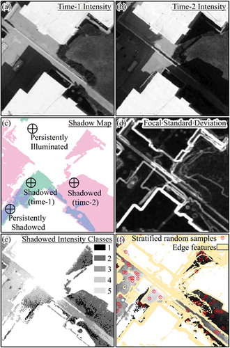
We observe that change detections are subject to errors from inaccurate co-registration, especially along edge gradients and in areas of high localized texture (cf. Dai and Khorram 1998). In order to improve the fidelity (i.e., accuracy and reliability) of samples used in the PIF-LR and RCS techniques, we pre-filtered the intensity images to reduce such artifacts. We estimated texture using focal standard deviation images (involving a 5-x-5 pixel kernel) derived from t-1 and t-2 intensity (Figure 4). Global mean values were computed for the standard deviation images (Figure 4-d). All pixels that exceeded these global mean values were classified and used to mask out the coincident pixels in the t-1 as well as t-2 intensity images. This procedure was effective for extracting regions of the images that exhibit relatively uniform texture. We then applied low-pass filters based on 5-x-5 kernels in order to further reduce potential image misalignment effects in the areas that were not masked out (Figure 4-f). Stratified random pixel sampling (described below) was applied to the edge-masked and low-pass-filtered regions, which represent PIFs for the purposes of this study. Because changes involving physical objects in the study images are not prevalent, we did not apply filters to preclude such changes from the radiometric samples. Such a step would be required for scenes containing substantial amounts of change.

Figure 4. Procedural steps for isolating invariant features within shadows to support radiometric normalization: (a and b) t-1 and t-2 intensity images containing transient shadows; (c) shadow map derived from intensity and intensity-normalized blue variations; (d) additive result of 5-x-5 focal standard deviation kernels applied to t-1 and t-2, enhancing edges; (e) stratification based on five equal-interval classes of the intensity range within transient shadows; and, (f) stratified random points (red circles) used to sample pixels from t-1 and t-2 intensity images that were edge-masked (yellow zones), and low-pass filtered using a 5-x-5 moving-average kernel.

Shadow normalization

We applied the four normalization approaches illustrated in Figure 1 to transient shadows in each of the bi-temporal image sets. The MV adjustments were based on Equation (1), and effectively increased the mean and variance values of all pixels in the transient shadow areas, in order to approximate D-I conditions. HM normalization was implemented using the Histogram Match operation in ERDAS Imagine™. The HM and MV normalizations were based on the entire set of transient S pixels in each image.

We employed a random sampling procedure to support the PIF-LR and RCS normalizations. Five sets of 30 random pixels (totaling 150) were generated using ESRI ArcMap™ within five strata of intensity associated with the transient shadows of each image (Figure 4-e and 4-f). The intensity strata were defined by equal intervals within the range of −2.0 to + 2.0 standard deviations from the mean intensity value for the transient shadows unique to each image. The stratified random sample pixels were used to extract intensity values from t-1 and t-2 for each scene, based on the edge-masked and low-pass-filtered images. In the PIF-LR approach, data from the 150-pixel sets were used to derive ordinary least-squares linear regressions using Excel™. Slope and intercept values derived from these regressions (having R² values of 0.55 to 0.99) were the basis for normalization. In the RCS approach, mean intensity values associated with the lowest and highest stratified pixel sample sets were used to define the radiometric control set values. The pixels with shadow-normalized values were then substituted for the corresponding pixels in the unnormalized intensity images. The equations used in the RCS and PIF-LR approaches are described by Yang and Lo (2000).

Post-processing

Forced allocation of pixel values into expanded bin ranges during histogram specification can lead to granulated patterns in image texture (cf. Cox, Roy, and Hingorani 1995). Similar artifacts can result from linear stretching of dynamic range (cf. Shor and Lischinski 2008). Therefore, we implemented a procedure (illustrated in Figure 5) to restore localized texture following the shadow normalizations. A low-pass filter was applied to the unnormalized intensity images (Figure 5-b), and we computed the pixel-wise difference between the low-pass images and the intensity images from which these were derived (Figure 5-d). This provided a localized measure of contrast for each pixel based in its neighbors’ intensity values. This measure was derived from the shadow-normalized and unnormalized intensities and arithmetically differenced as a metric of textural change, in units of pixel intensity. Finally, the pixel-specific texture change values were added to the normalized images as a means of restoring the original image texture. A minor disadvantage of this approach is that texture is altered along abrupt intensity gradients (Figure 5-e); a major advantage is the preservation of high-frequency intensity variations (Figure 5-f) that would be lost in a basic low-pass filtering operation (Figure 5-c).

Figure 5. Illustration of the texture restoration procedure applied to shadow-normalized intensity images: (a) unaltered intensity image containing shadow; (b) shadow-normalized product derived using the pseudo-invariant feature based linear regression (PIF-LR) technique; (c) unaltered intensity image after low-pass filtering with a 3-x-3 moving average kernel (low-pass filter was also applied to shadow-normalized image); (d) estimate of localized texture artifacts stemming from shadow normalization, based on contrast between the shadow-normalized and unaltered intensity images compared to low-pass filtered versions of each image (measuring changes in localized texture); texture differences were subtracted from shadow-normalized image; (e) difference in focal standard deviation (based on a 3-x-3 kernel) between the shadow-normalized intensity image; and (f) product of the shadow normalization and texture restoration procedures which preserves more detail than the low-pass filtered product.

Evaluation

Separate sets of randomly sampled pixels were used to evaluate shadow normalization results. Samples were stratified by five intervals of intensity within transient shadows of each image (n = 30 per interval). Effectiveness of the approaches was estimated in a direct manner based on intensity differences between the shadow-normalized products and the counterpart images, which represent D-I conditions. All intensity images used for evaluation were edge-masked and low-pass filtered for misregistration effects, and the points were visually screened to prevent sampling in misclassified shadow areas. Intensity variations within each image correspond mainly to differences of material type. We deemed intensity strata to be more appropriate than material type categories for comparing results, due to inter-scene differences of composition. Median and standard deviation values of intensity difference based on these samples capture the radiometric accuracy of the shadow-normalized products.

The Hospital Facility scene was selected for a qualitative evaluation of the practical utility of the shadow normalizations for the purpose of change detection, based on image differencing and visual inspection of features. This scene was chosen due to the prevalence of shadows and changed features within it. We derived arithmetical differences between the t-1 and t-2 images (shadow-normalized and unnormalized versions). The utility of the shadow-normalized products was evaluated according to the advantages provided (over the unnormalized images) for a semi-automated image pre-processing workflow, involving a human analyst who interprets the imagery and identifies changed features.

Results

We evaluate the shadow normalization results quantitatively, based on samples of shadow-normalized and unnormalized intensities at t-1 and t-2 (Figure 6). In all cases, the shadow normalizations increased the similarity of the intensity values to those associated with D-I conditions. The effectiveness of each shadow normalization approach varies among intensity strata in each scene. The levels of scatter represented by intensity standard deviation values are generally similar among the different approaches, and not substantially different from those observed in the unnormalized intensity samples. Specific results based on Figure 6 are summarized below according to scene. We use the term performance to describe how effectively the shadow normalizations are in rendering intensity values that approximate D-I conditions.

Figure 6. Bar charts used to evaluate the effectiveness of the shadow normalization approaches, based on random pixel samples which are stratified (n = 30) per five equal-intervals within the intensity range associated with transient shadow areas (shadowed condition) in each image. Bar values for the normalization results represent mean values of intensity difference compared to the directly-illuminated condition in the counterpart (unshadowed) images. The pixel samples were derived from normalized and original images which were low-pass filtered to reduce misalignment artifacts. Bars represent (1) standard deviation values associated with the samples. Figures (a) and (b) represent the Bridge Overpass scene at t-1 and t-2; (c) and (d) represent the Hospital Facility scene at t-1 and t-2; (e) and (f) represent the Office Park scene at t-1 and t-2.

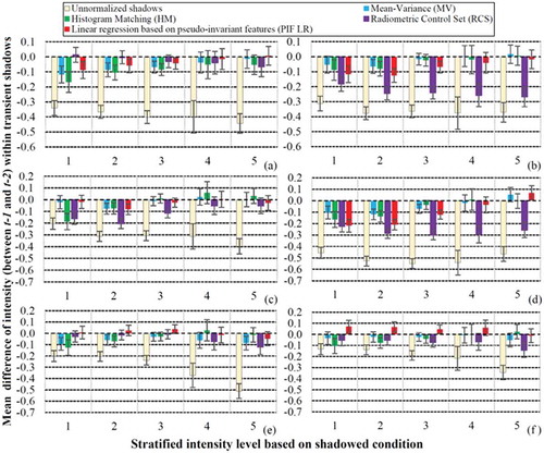
Bridge overpass

Performance of the different approaches varies substantially between t-1 (Figure 6a) and t-2 (Figure 6-b) for the Bridge Overpass scene. In t-1, the RCS and PIF-LR approaches exhibit superior performance, resulting in intensity variations of 0.05 to 0.10 from the D-I condition. Conversely, the HM and MV approaches exhibit superior performance in t-2, showing average intensity variations of less than 0.10 from the D-I condition. The RCS approach is least reliable among the different approaches tested for this scene, showing only minor differences from the unnormalized intensity levels within transient shadows at t-2. Based on the results from the MV, HM, and PIF-LR approaches, shadow normalization is most effective for the higher intensity classes (3 to 5) for this scene. This pattern may be attributable to higher precision of sensor response where surface radiance is higher.

Hospital facility

Performance of the different approaches does not vary substantially between t-1 (Figure 6-c) and t-2 (Figure 6-d) for the Hospital Facility scene, except with respect to the RCS approach. In t-1, the MV and PIF-LR approaches exhibit superior performance, resulting generally in intensity variations of less than 0.05 from the D-I condition. The MV approach also exhibits high performance in t-2, whereas the PIF-LR approach is less reliable in t-2. Generally, the performance of the HM approach co-varies with that of the MV approach in t-1 and t-2. Based on this scene, we observe a similar pattern of performance in the different approaches (according to intensity class) as with the Bridge Overpass scene, namely that normalization effectiveness is generally higher at greater intensity levels.

Office park

Performance of the different normalization approaches does not vary substantially between t-1 (Figure 6-e) and t-2 (Figure 6-f) for the Office Park scene. In t-1, the MV and PIF-LR approaches exhibit superior performance, generally resulting in intensity variations of less than 0.05 from the D-I condition. In contrast to the other scenes, Office Park shows no clear pattern of performance variability according to intensity level, except that the RCS approach shows lower performance in the higher intensity classes. Results from the PIF-LR approach exhibit a negative (under-brightening) bias in t-1, compared to a positive bias in t-2. Possible explanations for these biases and performance variations are discussed further below.

Aggregate-level results

A summary of the results from the 150 stratified random sample pixels in each image is given in Table 1. The MV approach represents the most effective normalization for the greatest number of images (3 of 6) as compared to the other approaches. Considering the mean absolute difference (based on all six sets of 150 pixels) the MV approach rendered intensity values that approximate the D-I condition within 0.049 intensity units (~ 5% of the dynamic range). This difference is slightly lower than observed from the approaches of HM (0.061) and PIF-LR (0.059). The RCS approach produced a mean absolute intensity difference of 0.131. The average levels of scatter (standard deviation) based on the aggregate level results are similar among the approaches (MV: 0.062, HM: 0.061, RCS: 0.060, PIF-LR: 0.065), and relative to the unnormalized samples (0.066).

Table 1. Aggregate mean values of intensity difference between t-1 and t-2, based on the stratified random samples used to evaluate results from the shadow normalization approaches. Mean values are derived from averages of absolute difference values (n = 150) from a merger of five intensity strata that are represented in Figure 6. The lowest values (corresponding to higher performance) among the different approaches are underlined.

Scene	Image	Unnormalized	MV	HM	RCS	PIF-LR
Bridge Overpass	time-1	0.390	0.065	0.093	0.031	0.043
	time-2	0.360	0.031	0.044	0.239	0.074
Hospital Facility	time-1	0.307	0.027	0.072	0.116	0.031
	time-2	0.508	0.074	0.071	0.273	0.131
Office Park	time-1	0.305	0.066	0.053	0.049	0.026
	time-2	0.205	0.028	0.050	0.078	0.051
Aggregate means:		0.346	0.049	0.064	0.131	0.059

Qualitative evaluation of shadow-normalized products for change detection

The practical reason for evaluating shadow normalizations in this study is that transient shadows represent a source of error in change detection based on image differencing and post-classification comparison. Low intensity in shadows can also hinder visual identification of features. In this context, we describe practical steps, uses of ancillary data sets, technical considerations, and limitations which were identified while using the shadow normalized products for change detection.

The unnormalized and shadow-normalized intensity images associated with the Hospital Facility scene are portrayed in Figure 7. Identical coefficients for mean and variance adjustment were applied to the transient and persistent shadow areas in this example. The normalizations greatly enhanced visibility of features within shadows, including motor vehicles and landscaped features near to the hospital. Such features can be readily compared to features in D-I areas. In this demonstration, shadow features having less than 10 m² in contiguous area were excluded from the normalization. Shadow penumbra were also masked out of the change detection product, in order to focus on spatial changes among physical features.

Figure 7. Hospital Facility scene example to illustrate the potential utility of shadow normalization for the purpose of change detection: (a) original intensity image at t-1; (b) shadow-normalized intensity image at t-1; (c) original intensity image at t-2; (d) shadow-normalized intensity image at t-2; (e) original t-2 intensity subtracted from original t-1 intensity (intensity difference); (f) shadow-normalized intensity difference image, wherein small shadows and penumbra areas are masked out in light blue; (g) difference of (t-1 and t-2) focal (5 X 5) standard deviation images based on unnormalized intensity, which reveal misalignment artifacts and changed features having linear boundaries; (h and i) the original true-color images, subset to frame extent and separated according to shadow zone to enhance brightness display, which allow visual identification of changed features (labelled in red).

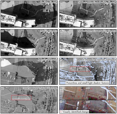
The shadow-normalized intensity difference image appears to have suppressed shadow effects and is a viable basis for visual discrimination of changed features. Several automobiles that changed in location are more clearly visible in the normalized than unnormalized difference image. The unnormalized difference image also shows false changes associated with geometric misalignments, including edges of the hospital building. The t-1 versus t-2 difference in focal standard deviation (Figure 7-e) proved useful for identifying geometric misalignments. The focal standard deviation difference also highlights shadow penumbra and abrupt gradients associated with changed features (such as automobiles) and facilitates change detection in this example.

We focused on an area of interest (AOI) which represents an appropriate frame scale for visual identification of small changes by a human analyst (Figure 7-f and 7-g). We subset the original RGB images to this AOI for the purpose of visual assessment (Figure 7-h and 7-i). The RGB images were also subset according to shadow class to improve display contrast. The result is a bi-temporal RGB image sub-frame which facilitates change detection. It was possible to quickly identify a total of 17 changed features within this AOI. In this case, visual identification of changes proved greatly more efficient and reliable than would have been possible based solely upon image differencing. The shadow classification and normalization procedures enabled us to identify the AOI, which was examined more closely based on color imagery with the aid of ancillary data layers.

Discussion and conclusion

The general objectives addressed in this study include: 1) apply radiometric normalization techniques (MV, HM, RCS, and PIF-LR) typically used for image-to-image normalization, for the novel purpose of normalizing transient shadows in multi-temporal high spatial resolution imagery; 2) evaluate transient shadow normalization results stemming from these techniques, based on reference images from which the D-I intensities are known; and, 3) evaluate the utility and limitations of the shadow-normalized intensity images for the purpose of change detection. Based on our quantitative assessment of the shadow-normalized products, each technique proved beneficial for reducing the radiometric effects of transient shadowing. Generally, the shadow normalizations reduced the radiometric effect of shadowing to less than 30 percent of that expressed in the unnormalized image sets (Table 1). The MV approach yielded the most effective normalizations, reducing the average shadowing effect from 0.346 to 0.049 intensity units (~ 85 percent reduction); similar results were obtained through the HM and PIF-LR approaches. The radiometric fidelity of the normalizations among intensity levels is an important quality, especially for change detection in scenes with mixed material types having unique reflectance properties. The MV approach shows the highest fidelity, while RCS approach exhibits relatively poor fidelity between intensity strata. The higher average performance of the PIF-LR approach compared to the RCS approach is attributed to greater representativeness of the t-1 to t-2 intensity relationships based on five versus only two intensity strata. The general finding that normalizations are more effective at higher intensity levels is consistent for the MV, HM, and PIF-LR approaches. This pattern may be attributable to higher radiometric resolution at higher radiance levels. A rigorous explanation of variations in performance by the normalization techniques would require an analysis to quantify the contributions of sampling, scene characteristics, illumination variability, and image misalignment (among other potential factors) to the observed errors.

This study clearly demonstrates the utility of image-to-image normalization for reducing the radiometric effects of transient shadows in aerial frame imagery. An important component of this study is the evaluation approach, which measured directly the correspondence of shadow-normalized and D-I intensities as shadow effect reduction (61–85 percent, depending on normalization approach). Guo, Dai, and Hoiem (2013) report 60–72 percent reductions in SR effects of shadowing, through comparison of shadow-normalized and reference images showing D-I conditions. However, their evaluation results are based on the L*a*b space (which combines intensity and color components) and may differ from our statistics that are based on intensity alone. It was beyond the scope of this study to compare results with those from the various other approaches evaluated by Gong and Cosker (2016), who report normalized metrics of similarity in “textureness,” “softness,” “brokenness,” and “colorfulness” (vis-à-vis reference or “ground truth” images), rather than radiometric units such as intensity. Based on our visual comparisons, shadow normalization products based on the techniques of Guo, Dai, and Hoiem (2013), Gong et al. (2013), and Gong and Cosker (2016) seem to have the highest aesthetic quality of any evaluated in the literature. However, the performance and efficiency of such methods with aerial images representing scenes that contain dozens of shadowed material types in complex arrangements are unknown, because testing was generally applied to simpler images containing few shadows and material types. These methods require parameterization and user-guided steps, and thus are incompatible with our ultimate objective of automation. Automated techniques proposed by Fredembach and Finlayson (2006), Finlayson, Drew, and Lu (2009), Salamati, Germain, and Siisstrunk (2011), Yang et al. (2012), and Khan et al. (2016) rely on illumination-invariant color spaces (e.g. chromaticity), directional entropy, or image matting. Such techniques are powerful, but the associated literature diverges markedly from that of multi-temporal remote sensing in practical context as well as terminology. Given the practical utility of multi-temporal remote sensing, we propose that future research on shadow normalization should involve comparison of multi-temporal images, based on spectral-radiometric attributes that are meaningful in scientific applications.

The metrics of shadow normalization performance used in this study are largely quantitative, whereas practical usefulness and limitations are best determined with respect to specific applications or change detection objectives. For example, classifying pixels that show greater than 0.10 variation in intensity (between t-1 and t-2) as changes would be an appropriate use of the shadow-normalized images based on the MV technique; using a variation threshold of 0.025 intensity units to classify changes would result in many false detections in shadow-normalized areas. Therefore, users should determine whether to apply the MV or other relative radiometric normalizations to reduce shadow artifacts by considering feature- and application-specific parameters such as post-hazard damage classification criteria.

Any shadow normalization is likely beneficial for change detection based on intensity differences, provided that the artifacts stemming from image misalignment and inaccuracy of shadow classification can be either resolved or precluded. The spatial scale of the features or changes of interest is a key factor to be considered in shadow normalization. In our demonstration, we masked out shadows that were likely too small to contain features of interest and that would lead to many penumbra artifacts following normalization. We found that supplementing the shadow normalized products with standard deviation difference images highlights potential misalignment artifacts, and that sub-setting the RGB images according to shadow class and AOI greatly facilitates change detection by a human analyst.

The shadow normalization approaches evaluated in this study represent one component of an integrated workflow for near-real-time change detection based on multi-temporal aerial frame imagery. Other vital components include efficient flight planning, repeat station image (RSI) acquisition to optimize image co-registration, automatable and accurate shadow detection, change detection, and effective digital communications that facilitate human decision-making. This study presents a novel approach to shadow normalization in a multi-temporal imaging context, one which can meet the requirements for near-real-time processing in time-sensitive applications including disaster response. Imperfect co-registration is likely to remain a key source of uncertainty and error in shadow detection, shadow normalization, and change detection based on multi-temporal aerial frame imagery. Follow-on research to improve multi-temporal image alignment, by applying shadow normalization to singular images prior to co-registration, should increase the effectiveness of this multi-faceted procedure to support detailed change detection in a near-real-time fashion. Improved capacity to normalize and detect changes within small shadows and penumbra based on relative radiometric adjustments would represent a major advancement in this research domain.

Acknowledgements

This study was funded primarily by the National Science Foundation Directorate of Engineering, Infrastructure Management and Extreme Events (IMEE) program (Grant # G00010529) and United States Department of Transportation (USDOT) Office of the Assistant Secretary for Research & Technology (OST-R) Commercial Remote Sensing and Spatial Information Technologies Program (CRS&SI), cooperative agreement # OASRTRS-14-H-UNM, and partially by the National Aeronautics & Space Administration (NASA) through a Earth & Space Science Fellowship training grant (# 80NSSC17K0393) supporting Emanuel Storey. Christopher Chen, Lloyd Coulter, Andrew Kerr, Garrick MacDonald, Eugene Schweizer, and Nicholas Zamora (SDSU), and Richard McCreight (NEOS, LTD) contributed to research components associated with this article.

Disclosure statement

No potential conflict of interest was reported by the authors.

Additional information

Funding

This work was supported by the National Aeronautics and Space Administration [80NSSC17K0393];National Science Foundation [G00010529];U.S. Department of Transportation [OASRTRS-14-H-UNM].

References

- Arbel, E., and H. Hel-Or. 2011. “Shadow Removal Using Intensity Surfaces and Texture Anchor Points.” IEEE Transactions on Pattern Analysis and Machine Intelligence 33 (6): 1202–1216. doi:10.1109/TPAMI.2010.157.
- Benediktsson, J. A., and J. R. Sveinsson. 1997. “Feature Extraction for Multisource Data Classification with Artificial Neural Networks.” International Journal of Remote Sensing 18 (4): 727–740. doi:10.1080/014311697218728.
- Chavez, P. S. 1975. “Atmospheric, Solar, and MTF Corrections for ERTS Digital Imagery.” In Paper Presented at the Fall Annual Meeting for the American Society of Photogrammetry, 459–479. Phoenix, AZ.
- Coppin, P. R., and M. E. Bauer. 1994. “Processing of Multitemporal Landsat TM Imagery to Optimize Extraction of Forest Cover Change Features.” IEEE Transactions on Geoscience and Remote Sensing 32 (4): 918–927. doi:10.1109/36.298020.
- Coulter, L., and D. Stow. 2005. “Detailed Change Detection Using High Spatial Resolution Frame Center Matched Aerial Photography.” In Paper Presented for the 20th Biennial Workshop on Aerial Photography, Videography, and High Resolution Digital Imagery for Resource Assessment, 4–8. Weslaco, TX.
- Coulter, L., D. Stow, S. Kumar, S. Dua, B. Loveless, G. Fraley, C. Lippitt, and V. Shrivastava. 2012. “Automated Co-Registration of Multitemporal Airborne Frame Images for near Real-Time Change Detection.” In Paper Presented at the Annual Meeting for the American Society for Photogrammetry and Remote Sensing, 19–23. Sacramento, CA.
- Coulter, L. L., and D. A. Stow. 2008. “Assessment of the Spatial Co-Registration of Multitemporal Imagery from Large Format Digital Cameras in the Context of Detailed Change Detection.” Sensors 8 (4): 2161–2173. doi:10.3390/s8042161.
- Coulter, L. L., D. A. Stow, C. D. Lippitt, and G. W. Fraley. 2015. “Repeat Station Imaging for Rapid Airborne Change Detection.” In Time-Sensitive Remote Sensing, edited by Lippitt, Christopher D., Douglas A . Stow, and Lloyd L . Coulter, 29–43. New York: Springer.
- Coulter, L. L., D. A. Stow, and S. Baer. 2003. “A Frame Center Matching Technique for Precise Registration of Multitemporal Airborne Frame Imagery.” IEEE Transactions on Geoscience and Remote Sensing 41 (11): 2436–2444. doi:10.1109/TGRS.2003.819191.
- Cox, I. J., S. Roy, and S. L. Hingorani. 1995. “Dynamic Histogram Warping of Image Pairs for Constant Image Brightness.” In Paper Presented for the Annual IEEE International Conference on Image Processing, 366–369. Washington, DC.
- Dai, X., and S. Khorram. 1998. “The Effects of Image Misregistration on the Accuracy of Remotely Sensed Change Detection.” IEEE Transactions on Geoscience and Remote Sensing 36 (5): 1566–1577. doi:10.1109/36.718860.
- Dalla Mura, M., J. A. Benediktsson, F. Bovolo, and L. Bruzzone. 2008. “An Unsupervised Technique Based OnMorphological Filters for Change Detection in Very High Resolution Images.” Ieee Geoscience and Remote SensingLetters 5 (3): 433–437. doi:10.1109/LGRS.2008.917726.
- Dare, P. M. 2005. “Shadow Analysis in High-Resolution Satellite Imagery of Urban Areas.” Photogrammetric Engineering & Remote Sensing 71 (2): 169–177. doi:10.14358/PERS.71.2.169.
- Drew, M. S., L. Cheng, and G. D. Finlayson. 2006. “Removing Shadows Using Flash/Noflash Image Edges.” In Paper Presented for the IEEE International Conference on Multimedia and Expo, 257–260. Toronto, Canada.
- Du, Y., P. M. Teillet, and J. Cihlar. 2002. “Radiometric Normalization of Multitemporal High-Resolution Satellite Images with Quality Control for Land Cover Change Detection.” Remote Sensing of Environment 82 (1): 123–134. doi:10.1016/S0034-4257(02)00029-9.
- Elvidge, C. D. 1995. “Relative Radiometric Normalization of Landsat Multispectral Scanner (MSS) Data Using an Automatic Scattergram-Controlled Regression.” Photogrammetric Engineering and Remote Sensing 61 (10): 1255–1260.
- Finlayson, G. D., M. S. Drew, and C. Lu. 2009. “Entropy Minimization for Shadow Removal.” International Journal of Computer Vision 85 (1): 35–57. doi:10.1007/s11263-009-0243-z.
- Fischler, M. A., and R. C. Bolles. 1981. “Random Sample Consensus: A Paradigm for Model Fitting with Applications to Image Analysis and Automated Cartography.” Communications of the ACM 24 (6): 381–395. doi:10.1145/358669.358692.
- Fredembach, C., and G. Finlayson. 2006. “Simple Shadow Removal.” In Paper Presented for the IEEE 18th International Conference on Pattern Recognition, 832–835. Hong Kong, China.
- Gong, H., and D. Cosker. 2016. “Interactive Removal and Ground Truth for Difficult Shadow Scenes.” Journal of the Optical Society of America. A, Optics, Image Science, and Vision 33 (9): 1798–1811.
- Gong, H., D. Cosker, C. Li, and M. Brown. 2013. “User-Aided Single Image Shadow Removal.” In Paper Presented for the IEEE International Conference on Multimedia and Expo, 1–6. San Jose, CA.
- Guo, R., Q. Dai, and D. Hoiem. 2011. “Single-Image Shadow Detection and Removal Using Paired Regions.” In Paper Presented for the IEEE Annual Conference on Computer Vision and Pattern Recognition, 2033–2040. Jodhpur, India.
- Guo, R., Q. Dai, and D. Hoiem. 2013. “Paired Regions for Shadow Detection and Removal.” IEEE Transactions on Pattern Analysis and Machine Intelligence 35 (12): 2956–2967. doi:10.1109/TPAMI.2012.214.
- Hall, F. G., D. E. Strebel, J. E. Nickeson, and S. J. Goetz. 1991. “Radiometric Rectification: Toward a Common Radiometric Response among Multidate, Multisensor Images.” Remote Sensing of Environment 35 (1): 11–27. doi:10.1016/0034-4257(91)90062-B.
- Jensen, J. R. 2009. Remote Sensing of the Environment: An Earth Resource Perspective 2/E. India: Pearson Education.
- Khan, S. H., M. Bennamoun, F. Sohel, and R. Togneri. 2016. “Automatic Shadow Detection and Removal from a Single Image.” IEEE Transactions on Pattern Analysis and Machine Intelligence 38 (3): 431–446. doi:10.1109/TPAMI.2015.2462355.
- Laliberte, A. S., D. M. Browning, and A. Rango. 2012. “A Comparison of Three Feature Selection Methods for Object-Based Classification of Sub-Decimeter Resolution UltraCam-L Imagery.” International Journal of Applied Earth Observation and Geoinformation 15: 70–78. doi:10.1016/j.jag.2011.05.011.
- Li, H., L. Zhang, and H. Shen. 2014. “An Adaptive Nonlocal Regularized Shadow Removal Method for Aerial Remote Sensing Images.” IEEE Transactions on Geoscience and Remote Sensing 52 (1): 106–120. doi:10.1109/TGRS.2012.2236562.
- Lippitt, C. D., and D. A. Stow. 2015. “Remote Sensing Theory and Time-Sensitive Information.” In Time-Sensitive Remote Sensing, edited by Lippitt, Christopher D., Douglas A . Stow, and Lloyd L . Coulter, 1–10. New York: Springer.
- Liu, F., and M. Gleicher. 2008. “Texture-Consistent Shadow Removal.” In Paper Presented for Annual Meeting of the European Conference on Computer Vision, 437–450. Marseille, France.
- Liu, W., and F. Yamazaki. 2012. “Object-Based Shadow Extraction and Correction of High-Resolution Optical Satellite Images.” IEEE Journal of Selected Topics in Applied Earth Observations and Remote Sensing 5 (4): 1296–1302. doi:10.1109/JSTARS.2012.2189558.
- Lowe, D. G. 2004. “Distinctive Image Features from Scale-Invariant Keypoints.” International Journal of Computer Vision 60 (2): 91–110. doi:10.1023/B:VISI.0000029664.99615.94.
- Robinson, B. F., and L. L. Biehl. 1982. “Calibration Procedures for Measurement of Reflectance Factor in Remote Sensing Field Research.” In Technical Report for Purdue University, Laboratory for Applications of Remote Sensing, 435–440. West Lafayette, Indiana.
- Salamati, N., A. Germain, and S. Siisstrunk. 2011. “Removing Shadows from Images Using Color and Near-Infrared.” In Paper Presented for the IEEE 18th International Conference on Image Processing, 1713–1716. Brussels, Belgium.
- Sanin, A., C. Sanderson, and B. C. Lovell. 2012. “Shadow Detection: A Survey and Comparative Evaluation of Recent Methods.” Pattern Recognition 45 (4): 1684–1695. doi:10.1016/j.patcog.2011.10.001.
- Schott, J. R., C. Salvaggio, and W.J. Volchok. 1988. “Radiometric Scene NormalizationUsing Pseudoinvariant Features.” Remote Sensing Of Environment 26 (1): 1–16. doi:10.1016/0034-4257(88)90116-2.
- Shor, Y., and D. Lischinski. 2008. “The Shadow Meets the Mask: Pyramid-Based Shadow Removal.” Computer Graphics Forum 27 (2): 577–586. doi:10.1111/j.1467-8659.2008.01155.x.
- Shu, J. S.-P., and H. Freeman. 1990. “Cloud Shadow Removal from Aerial Photographs.” Pattern Recognition 23 (6): 647–656. doi:10.1016/0031-3203(90)90040-R.
- Silva, G. F., G. B. Carneiro, R. Doth, L. A. Amaral, and D. F. G. De Azevedo. 2017. “Near Real-Time Shadow Detection and Removal in Aerial Motion Imagery Application.” ISPRS Journal of Photogrammetry and Remote Sensing. doi:10.1016/j.isprsjprs.2017.11.005.
- Slater, P. N., S. F. Biggar, R. G. Holm, R. D. Jackson, Y. Mao, M. S. Moran, and B. Yuan. 1987. “Reflectance-and Radiance-based Methods for The In-flight Absolute Calibration Of Multispectral Sensors.” Remote Sensing Of Environment 22 (1): 11–37.
- Song, C., C. E. Woodcock, K. C. Seto, M. P. Lenney, and S. A. Macomber. 2001. “Classification and Change Detection Using Landsat TM Data: When and How to Correct Atmospheric Effects?” Remote Sensing of Environment 75 (2): 230–244. doi:10.1016/S0034-4257(00)00169-3.
- Storey, E. A., D. A. Stow, L. L. Coulter, and C. Chen. 2017. “Detecting Shadows in Multi-Temporal Aerial Imagery to Support Near-Real-Time Change Detection.” GIScience & Remote Sensing 54 (4): 453–470.
- Stow, D., L. Coulter, and S. Baer. 2003. “A Frame Centre Matching Approach to Registration for Change Detection with Fine Spatial Resolution Multi-Temporal Imagery.” International Journal of Remote Sensing 24 (19): 3873–3879.
- Stow, D. A., L. C. Coulter, G. MacDonald, C. D. Lippitt, R. McCreight, and N. Zamora. 2016. “Evaluation of Geometric Elements of Repeat Station Imaging and Registration.” Photogrammetric Engineering & Remote Sensing 82 (10): 775–788.
- Turner, D., A. Lucieer, Z. Malenovský, D. H. King, and S. A. Robinson. 2014. “Spatial Co-Registration of Ultra-High Resolution Visible, Multispectral and Thermal Images Acquired with a micro-UAV over Antarctic Moss Beds.” Remote Sensing 6 (5): 4003–4024.
- Wang, B., A. Ono, K. Muramatsu, and N. Fujiwara. 1999. “Automated Detection and Removal of Clouds and Their Shadows from Landsat TM Images.” IEICE Transactions on Information and Systems 82 (2): 453–460.
- Xiao, C., R. She, D. Xiao, and M. Kwan‐Liu. 2013. “Fast Shadow Removal Using Adaptive Multi‐Scale Illumination Transfer.” Computer Graphics Forum 32 (8): 207–218.
- Yang, Q., K-H. Tan, and N. Ahuja. 2012. “Shadow Removal Using Bilateral Filtering.” IeeeTransactions on Image Processing 21 (10): 4361–4368. doi:10.1109/TIP.2012.2208976.
- Yang, X., and C. P. Lo. 2000. “Relative Radiometric Normalization Performance for Change Detection from Multi-Date Satellite Images.” Photogrammetric Engineering and Remote Sensing 66 (8): 967–980.
- Zhang, L., Q. Zhang, and C. Xiao. 2015. “Shadow Remover: Image Shadow Removal Based on Illumination Recovering Optimization.” IEEE Transactions on Image Processing 24 (11): 4623–4636.