Examining deforestation and agropasture dynamics along the Brazilian TransAmazon Highway using multitemporal Landsat imagery

Abstract

This research aims to understand the difference of major land-cover change results caused in various time periods and to examine the impacts of human-induced factors on land-cover changes along the TransAmazon Highway region. The Landsat Thematic Mapper and Operational Land Imager data from 2011, 2014, and 2017 and our previous land-cover classification results in 1991, 2000, and 2008 were used to examine land-cover dynamics. A classification system consisting of five land-cover classes – primary forest (PF), secondary forest (SF), agropasture (AP), urban area, and water – were chosen. The hierarchical-based classification method was used to generate land-cover classification results, and the post-classification comparison approach was used to produce detailed “from-to” conversions for each detection period. The emphasis was on deforestation of PF, dynamic change of SF and AP, and urbanization over time. The impacts of human-induced factors such as population and economic conditions on urban expansion, AP expansion, and deforestation were examined. This research indicated that selection of a suitable time period was critical for effectively detecting land-cover changes; that is, too long time period (i.e., 9 years) cannot accurately capture some land-cover changes such as the AP and SF in this research. Although deforestation – the conversion from PF to SF and AP – accounted for a large proportion of land-cover changes, the changes between SF and AP became more important than PF conversion, and required a short time period (i.e., 3 years here) for effectively reflecting their dynamics. Human-induced factors play important roles in deforestation, dynamic changes between AP and SF, and urbanization.

Keywords:

• deforestation
• secondary forest
• agropasture expansion
• TransAmazon
• multitemporal Landsat imagery
• human-induced factors

1. Introduction

Deforestation in the TransAmazon region in the eastern Amazon began in the 1970s due to the construction of highways and rural settlements that attracted the migration of populations from southern parts of Brazil (Moran 1975, 1981; Moran and Brondizio 1998). Thousands of small farmers were attracted to the region with support from the Brazilian government and received parcels of 100 hectares of land, financing, technical assistance, and other incentives to occupy the region and start agropastoral activities (Moran 1981), resulting in rapid agricultural expansion and extensive livestock farming (Walker, Moran, and Anselin 2000; Lu et al. 2013; Brazilian Government 2017). The recent expansion of urban areas and the population growth caused by the construction of large infrastructure projects (e.g., Belo Monte Dam, about 50 km from Altamira) can enhance the impact of human actions on agroecosystems (Tundisi, Matsumura-Tundisi, and Tundisi 2015; Fearnside 2016; Moran 2016; Atkins 2017; Ritter et al. 2017). In this region, the agropastoral activities were mainly due to traditional systems of slash-and-burn agriculture and increased by expansion into new areas of forest (Walker, Moran, and Anselin 2000). Large areas of primary forests were replaced by pastures, agricultural lands, and cocoa plantations or secondary forests (Lu et al. 2013).

Deforestation has been regarded as an important factor resulting in environmental problems such as land degradation (Walker and Homma 1996). Many studies have been conducted in the Brazilian Amazon to examine the deforestation, forest degradation and restoration, as well as the agricultural and pastoral expansions (Lu et al. 2013; Spera et al. 2014; Chen et al. 2015; Imbach et al. 2015; Müller, Griffiths, and Hostert 2016; Grecchi et al. 2017). Remote sensing technology has long been used for detecting deforestation because it can acquire data repeatedly with large coverage, especially when long-term Landsat images are available at no cost (Brondízio 2005; Schneibel et al. 2017; Shimizu et al. 2017). Therefore, much research explored the approaches to accurately detect the changes in different land covers (Lu et al. 2004c; Grecchi et al. 2014; Lu, Li, and Moran 2014; Beuchle et al. 2015; Silveira et al. 2018). Grecchi et al. (2014) conducted research on land-use and land-cover changes and their impact on the environment in southeast Mato Grosso State based on Landsat, MODIS, and elevation data using post-classification comparison methods, and found that during 1985–1995, crops (rice and soy bean) expanded at high rates, and a large part of Cerrado, Brazil’s tropical savanna ecoregion, was converted to agriculture. After 1995, crops continued to expand and encroached into fragile environments such as wetlands and more erodible soils. Between 1985 and 2005, approximately 42% of predominantly vegetated area was lost to agriculture, and soil erosion increased significantly. Silveira et al. (2018) developed a new method for detecting seasonal changes in Brazilian savannahs. This method used an object-based approach to extract geostatistical features from bitemporal Landsat Thematic Mapper (TM) images (wet and dry seasons). The results indicated that change detection accuracies have been greatly improved by using the most geostatistical features compared with the spectral features and image differencing technique.

In general, most change detection studies cover two broad categories: selection of suitable remote sensing parameters and use of proper algorithms. The parameters can be pixel-based, object-based (e.g., image segmentation based on high spatial resolution images), and subpixel-based (fractional images) (Lu, Li, and Moran 2014). The change detection algorithm can also be separated into two broad categories: detecting the binary change and non-change and detecting the detailed change trajectories. Most of the change detection techniques such as principal component analysis and image differencing can only detect change and non-change information using the thresholding-based approach (Lu et al. 2004c). However, the change and non-change information cannot provide sufficient information required for particular purposes (e.g., driving forces of deforestation, land-cover and land-use change modelling); detailed change trajectories are often needed, for which the post-classification comparison approach is commonly used (Lu et al. 2013). The post-classification comparison method involves classification of individual images into land-cover maps at multitemporal scale and comparison of classified land-cover maps pixel by pixel. This method provides detailed “from-to” change trajectories and identifies where the change occurred and how much change occurred. The accuracy of change detection is dependent on the accuracy of each individual classification. However, every error in the individual classification map will be carried over into the final change detection. Thus, caution must be taken to ensure that all individual classifications are as accurate as possible.

In addition to the selection of suitable remote sensing data and algorithms, determination of suitable time periods is an important concern for effectively obtaining the needed change information. A long time period may hide the real changes, while a short time period may not capture the changes. One objective of this research was to understand the effects of different time periods in reflecting change detection results; thus, we compared the spatial patterns of deforestation and agropasture dynamic changes at nine(or eight)-year intervals (1991–2000–2008–2017) and at three-year intervals (2008–2011–2014–2017). Another objective was to examine the human-induced activities on these changes along the TransAmazon Highway region and the potential impacts of Belo Monte dam construction on deforestation and agropasture expansion in an area not directly affected by the construction but indirectly affected by the growth of population, loss of farm workers to dam construction, and the absence of policies directed at the agrarian sector during this period.

2. Study area

The study area is located in the northern Brazilian state of Pará (Figure 1), covering about 6,500 km² along the TransAmazon Highway (BR-230), which was inaugurated in 1972. Three cities – Altamira, Brasil Novo, and Medicilândia – are located along the highway in our study area. Altamira lies on Xingu River at the eastern edge of the study area, and Medicilândia is 90 km west of Altamira, while Brasil Novo is between them. The TransAmazon Highway construction and the accompanying colonization projects stimulated a large migratory influx to this area, resulting in extensive deforestation during the past four decades. At the east end of this study area is Xingu River with the Belo Monte hydroelectric dam, which was begun in 2011 and finished in 2016. Because of the dam construction, large numbers of people moved to Altamira and nearby construction sites, resulting in expanded urbanization (Feng et al. 2017).

Figure 1. Study area: Altamira TransAmazon Highway region, Pará State, Brazil, and Xingu River, highlighting Belo Monte Dam.

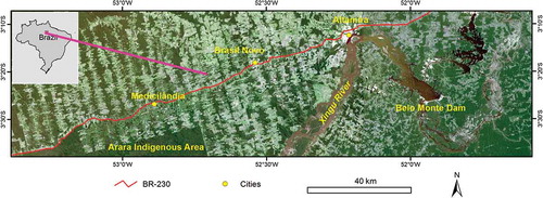
A large area of primary forests has been converted to successional vegetation, pasture, and agricultural lands since the early 1970s (Moran et al. 1994; Moran and Brondizio 1998; Lu et al. 2013). Cocoa plantations and livestock are the most important economic activities in this region. The cocoa plantations are commonly located in areas of Nitisols and Ferralsols and cultivated under agroforestry systems, resulting in complex forest structures in density and canopy strata (Calvi 2009). The yellow-colored Ferralsols areas (the most abundant soils in the region) are mainly used for the cultivation of pastures for raising cattle. Annual crops are grown at a reduced scale, usually at an early stage or concomitant with the planting of cocoa or pasture.

The study area is characterized by moderately rolling uplands with the highest elevation of approximately 350 m. The area has tropical climate with average annual temperature of 26ºC degrees and average annual precipitation of 2000 mm (Tucker, Brondizio, and Morán 1998). The temperature varies little throughout the year, but precipitation has significant seasonal variation, and most precipitation occurs from late October to early June.

3. Materials and methods

3.1. Data collection and preprocessing

The data used in this study are summarized in (Table 1). Multitemporal Landsat TM and Operational Land Imager images (path/row 226/62) covering 2011, 2014, and 2017 were used to develop land-cover distribution and dynamics. All Landsat images were atmospherically calibrated using the improved image-based dark object subtraction method (Chávez 1996; Chander, Markham, and Helder 2009) and co-registered to the Universal Transverse Mercator coordinate system. The root mean squared errors for the georegistration were less than 0.5 pixels, ensuring their geometric accuracy for change detection. Our previous research conducted land-cover classification using the Landsat TM images, and the results in 1991, 2000, and 2008 were directly used in this research (Lu et al. 2013). The Satellite Pour l’Observation de la Terre (SPOT-6) imagery, which was acquired on 19 August 2015, was used here for collection of different land-cover samples in rural areas for classification accuracy assessment. Since the SPOT image has four multispectral bands with 6 m spatial resolution and one panchromatic band with 1.5 m spatial resolution, the Gram-Schmidt Pan Sharpening approach was used to integrate both multispectral and panchromatic data into a newly fused multispectral image with improved spatial resolution for better visual interpretation performance (Karathanassi, Kolokousis, and Ioannidou 2007).

Table 1. Datasets used in research.

Dataset	Sources and dates
Landsat images	(1) Landsat 5 TM on 27 July 2011 (2) Landsat 8 OLI image on 20 August 2014 (3) Landsat 8 OLI images on June 16 and 11 July 2017 Spectral bands of blue, green, red, near infrared, and two short wavelength infrared from Landsat TM and OLI were used to develop land-cover maps
Land-cover images	Land-cover classification results were developed from Landsat TM images in 1991, 2000 and 2008 and were directly used in this research. The detailed descriptions of these classification results are provided in Lu et al. (2013).
SPOT 6	Satellite Pour l’Observation de la Terre (SPOT 6) imagery on 19 August 2015, was used for collection of land-cover samples.
Fieldwork	Different land-cover data were collected in January–May 2015
Roads	The roads were digitized from Google Earth images
Population GDP Herds of cattle	Data downloaded from Instituto Brasileiro de Geografia e Estatística for different years

Note: GDP, gross domestic product; TM, Thematic Mapper; OLI, Operational Land Imager

The field survey of land-cover types in this study area was conducted in January–May 2015 and covered the region between Altamira and Medicilândia. The field survey mainly collected sample plots of different land-cover types including different stages of secondary forest, pasture, and crop fields in rural areas and different urban land covers in Altamira. The sample plots’ locations were recorded with a Global Positioning System device. These field survey data and the collected samples from the 2015 SPOT fused imagery provided the basic source for selection of training and validation samples. In addition to remote sensing and field survey data, population, gross domestic product (GDP), and number of cattle herds were collected from Instituto Brasileiro de Geografia e Estatística (IBGE) to examine their impacts on deforestation and agropasture dynamics in this study.

3.2. Land-cover classification and accuracy assessment

Based on the research objectives, the characteristics of the study area, availability of reference data (field survey), selected remotely sensed data, and previous land-cover classification (Lu et al. 2013), a classification system consisting of five land-cover classes – primary forest (PF), secondary forest (SF), agropasture (AP), urban (UR), and water (WA) – was designed. In this study area, cocoa plantations have expanded rapidly in recent years due to cocoa’s high economic value. Based on our field survey in 2015, cocoa was planted in various densities and in mixture with other tree species, and its stand structure is very similar to SF, resulting in similar spectral features in Landsat imagery. Because of the difficulty in distinguishing SF and cocoa plantation using Landsat imagery, they were grouped into one SF category in this research. An additional class called cloud/shadow appeared in preliminary land-cover results of some years when clouds/shadows were not removed completely, even when using multiple image replacements. However, this class was removed from the final land-cover results after post-processing procedures by carefully examining the land-cover change patterns and designing logical change rules.

Our previous research on land-cover classification in the Brazilian Amazon had conducted a comprehensive comparison of different classification methods including maximum likelihood, classification tree, artificial neural network, k-nearest neighbor, and support vector machine using different remotely sensed data (e.g., Landsat, RADARSAT, ALOS PALSAR) (see Lu et al. 2004b; Li et al. 2011, 2012; Lu, Li, and Moran 2014). These methods require training samples during image classification, which were not available for historical remote sensing data. Therefore, we explored the hierarchical-based approach for land-cover classification in the Amazon basin (Lu et al. 2012). The method does not require field survey data as training samples. It has proved to be valuable when reference data are not available for historical remotely sensed data. The accuracy assessment results indicated that the hierarchical-based approach can provide better classification accuracy than other approaches, and this approach was used for land-cover classifications in three study areas in the Amazon (Lu et al. 2013), including part of the same study area (i.e., Altamira) as this research.

(Figure 2) illustrates the modified hierarchical classification. This method involved stratification and cluster analysis. UR was first extracted from Landsat multispectral images using a combination of thresholding, cluster analysis, and manual editing. The threshold of 0.4 based on high-albedo and low-albedo objects was used to produce the initial UR class (Lu et al. 2010). The spectral signatures of this initial UR class were extracted, and cluster analysis was used to classify these pixels into 30 clusters. The analyst merged the cluster into UR and other to improve the UR extraction accuracy. As shown in (Figure 2), UR was masked from the Landsat imagery, PF was then extracted from Landsat multispectral images using the combination of thresholding on a normalized difference vegetation index image and cluster analysis. The same procedure was used to extract WA, SF, and AP. After masking the extracted land-cover classes from Landsat imagery, some pixels still could not be directly extracted using the above procedure. The remaining pixels were classified into 50 clusters using cluster analysis. Each cluster was carefully examined with the assistance of the 2015 field survey data and labeled as one of the predefined land-cover types. This hierarchical-based classification method was used for generating preliminary land-cover classification results for 2011, 2014, and 2017.

Figure 2. The modified strategy for mapping land-cover distribution from Landsat imagery using the hierarchical-based approach (Note: TM, Thematic Mapper; NDVI, normalized difference vegetation index; MNDWI, modification of normalized difference water index; SF, secondary forest; AP, agropasture).

Due to spectral similarity between land-cover classes such as UR and AP, and PF and SF, misclassification is inevitable during the classification process. Expert rules based on comparison of multitemporal land-cover images and logical reasoning were used on the initial land-cover results to refine the land covers. The major rules and refinements are listed below:

1. Majority filter: Majority filter function with a window size of 3 × 3 pixels was applied to initial land-cover classification images of each time period to eliminate isolated pixels and reduce the salt-and-pepper problem in the classified image.

2. Manual editing: Clouds/shadows were superimposed onto the original Landsat image of 2014 with images from 2011 and 2017 side by side. By visual examination and manual interpretation, the clouds/shadows pixels were re-assigned to appropriate land-cover classes.

3. Automatic replacement: In reality, once PF land is cleared out, it has little or no chance to return to PF but can convert to other types of land cover; in contrast, once UR is established, it has little possibility to convert to other land-cover types. Based on these assumptions, the following automatic replacement rules were created: If pixels in the prior-date classification image were classified as SF, but they were classified as PF in the posterior-date image, these pixels in the posterior-date image were re-assigned to SF; if pixels in the prior-date classification image were classified as UR but were classified as AP in the posterior-date classification image, these pixels were re-assigned to UR in the posterior-date classification image, except the buildings and roads in flooding regions.

After the post-refining process on all land-cover maps of different years, the multitemporal land-cover images were generated. Ideally, the land-cover image of every time period needs to undergo accuracy assessment. However, the only available field data were collected in 2015. Thus only the 2014 classification result was evaluated, and classifications in 2011 and 2017 were not assessed due to lack of concurrent ground truth. Besides the sample plots collected from the field in 2015, we also collected samples from the pan-sharpened SPOT image. A total of 266 samples were used to assess the accuracy of the 2014 classification. An error matrix was produced, and overall accuracy, kappa coefficient, producer’s accuracy, and user’s accuracy were calculated (Foody 2002; Congalton and Green 2009).

3.3. Analysis of land-cover dynamic changes

The area of each land-cover class at each time point was calculated based on a classified image, and percentages of corresponding land covers accounting for the whole study area were also computed. The annual land-cover change is the changed area of each land-cover type between two dates divided by the number of years within the detection period. These results can provide general gains or losses of land-cover types, but they are not able to provide detailed land-cover conversion information. Therefore, the post-classification comparison approach was conducted, producing a two-way conversion matrix and areas of detailed “from-to” conversions for each detection period. In particular, the emphasis was on PF deforestation (conversion of PF to other land-cover types), dynamic change of SF and AP (loss/gain of SF and AP), and urbanization over time.

Pairwise comparison of land covers at two dates is efficient for identifying the changes in short time periods. For longer time periods, it underestimates the extent of land-cover change because it does not count the reversion changes occurring along the time course. For example, SF in the earliest investigation date may convert to AP at one time point, and later on, AP may change back to SF. Those changes cannot be detected and mistakenly identified as unchanged. Our field work in 2015 confirmed that some pasture lands were converted to cocoa plantations in recent years. To better reveal the extent of land-cover change, we combined the land-cover maps of all dates and extracted the pixels where the land-cover types never changed during the entire time period of 1991–2017, and calculated unchanged area for each land-cover type. The remaining pixels were those in which land-cover type changed at least once. For each land-cover type, the changed area was obtained by subtracting unchanged area from the area of corresponding land-cover type in 1991.

3.4. Examining impacts of human-induced factors on deforestation and agropasture dynamics

Land-cover change is the result of complex interactions of various biophysical and societal factors. Based on population and economic data collected from IBGE, the impacts of population and economic conditions (i.e., GDP) on urban expansion, AP expansion, and deforestation were examined. Meanwhile, the relationship between the total cattle herd and areas of AP was analyzed using linear and nonlinear regression. The interrelationships among different land-cover types, particularly urban growth, deforestation of PF, AP expansion, and deforestation of SF were also explored. Policies implemented and events occurring during a certain time period that might cause land-cover change were also discussed.

4. Results

4.1. Analysis of land-cover distribution and dynamic change

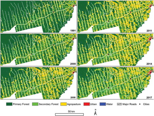
The overall accuracy of 83.4% and a kappa coefficient of 0.79 for the 2014 Landsat imagery were obtained (Table 2), an accuracy similar to the 2008 classification result using the hierarchical-based approach (Lu et al. 2013), indicating the robustness and reliability of this classification approach. As summarized in (Table 2), the major confusion was SF because advanced succession had stand structure similar to PF, and initial succession had spectral signatures similar to degraded pastures, resulting in relatively poor producer’s and user’s accuracies. (Figure 3) provides the spatial patterns of different land-cover distribution from 1991 to 2017. In 1991, PF dominated the study area, especially in the northwest and south of the study area, while in 2017, a large area was deforested and only limited PF remained in the northwest part. SF was mainly distributed along the highway and secondary roads, and limited AP was distributed around Altamira in 1991. Later on, SF became commonly distributed around Medicilândia, and AP around Altamira and Brasil Novo.

Table 2. Accuracy assessment result of the 2014 land-cover classification imagery.

Type	Reference data					RT	CT	UA	PA	Accuracy
	PF	SF	AP	UR	WA
PF	48	10				58	54	82.8	88.9	Overall accuracy: 83.4%; Kappa coefficient: 0.78
SF	4	54	11			69	76	78.3	71.1
AP		9	70			79	86	88.6	81.4
UR		1	5	24		30	24	80.0	100.0
WA	2	2			26	30	26	86.7	100.0

Note: PF, primary forest; SF, secondary forest; AP, agropasture; UR, urban; WA, water; RT, row total; CT, column total; UA, user’s accuracy; PA, producer’s accuracy.

Figure 3. Land-cover distributions at different years between 1991 and 2017.

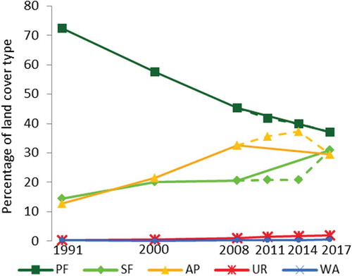
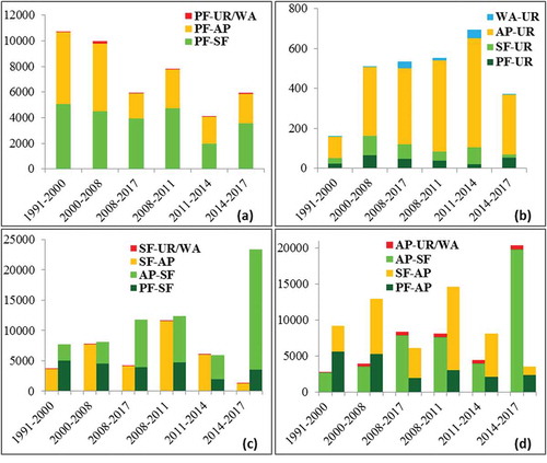
The trends of percentage change of different land-cover types over time (Figure 4) indicate that PF almost linearly decreased from 72.4% (470,925 ha) in 1991 to only 37.1% in 2017 (241,637 ha). SF increased slightly between 1991 and 2000, remained stable between 2000 and 2014, and then increased rapidly between 2014 and 2017. AP was continuous and linearly increased from 12.7% in 1991 (82,491 ha) to 37.4% in 2014 (243,122 ha), then decreased from 2014 to 2017. UR increased linearly by small percentages. Water accounted for a very small proportion in all time intervals. These results show that a long detection period may hide some internal change, especially for the land covers having frequent change such as SF and AP in this research. For example, between 2008 and 2017, SF increased from 20.5% to 30.9%, but most of this change occurred between 2014 and 2017, and there was almost no change in 2008–2011 and 2011–2014. AP decreased slightly from 32.7% in 2008 to 29.6% in 2017, but AP still linearly increased from 2008 to 2011 and to 2014, then sharply decreased from 37.4% in 2014 to 29.6% in 2017. This situation implies the importance of selecting suitable change detection periods for accurately extracting the real land-cover changes.

Figure 4. Proportion of land-cover types over time: a comparison of land-cover trends between 1991 and 2017 at nine-year intervals (solid lines) and between 2008 and 2017 at three-year intervals (dashed lines) (Note: PF, primary forest; SF, secondary forest; AP, agropasture; UR, urban; WA, water; percent of a land cover type = (A_i/A)*100, where A_i is the total area of the ith land-cover type and A is the total study area).

Considering all land covers from six dates between 1991 and 2017, only 47.4% of the study area did not change and 52.6% of areas changed at least once (Table 3): 48.7% of PF was irreversibly converted to other land-cover types, 67.2% of SF and 59.1% of AP changed one or more times. Almost all of the urban lands in 1991 still remained UR in 2017 due to the fact that once UR is developed, rarely can it be changed back to other land-cover types such as vegetation, unless a whole neighborhood is abandoned. Although 67.5% of water surface was detected as changed, it may be because the water table fluctuations in reservoirs and rivers in different years might cause misclassification of water and other land-cover types in the lowlands and floodplains.

Table 3. Summary of unchanged land-cover types between 1991 and 2017 and the land-cover types that changed at least once based on the 1991 land-cover data.

Type	Area in 1991 (ha)	Unchanged land covers between 1991 and 2017		Land covers that changed at least once based on the 1991 data
		Area (ha)	Percent	Area (ha)	Percent
PF	470,925	241,368	51.3	229,557	48.7
SF	94,162	30,888	32.8	63,274	67.2
AP	82,491	33,766	40.9	48,725	59.1
UR	1,788	1,773	99.2	15	0.8
WA	1,280	416	32.5	864	67.5
Total	650,645	308,211	47.4	342,434	52.6

Note: PF, primary forest; SF, secondary forest; AP, agropasture; UR, urban; WA, water

The annual land-cover change at different change detection periods (Figure 5) indicates that the long time period (9 years) and short time period (3 years) can provide very different conclusions. For example, PF had lower annual deforestation area in 2008–2017 than in 1991–2000 and 2000–2008, but within 2008–2017, the period of 2008–2011 had much higher annual deforestation than 2011–2014. For SF, the period of 2008–2017 had the highest annual increased area and the period of 2000–2008 had the lowest, but the increase in SF area occurred mainly in 2014–2017. On the other hand, AP decreased during 2008–2017, but two other periods of 1991–2000 and 2000–2008 showed increases. The decreased area was due to the large area lost in 2014–2017, but the areas increased in 2008–2011 and 2011–2014. UR had the highest increased area in 2011–2014, and water had the highest increased area in 2014–2017. The rapidly increased urban area in 2011–2014 and rapidly increased water area in 2014–2017 were coincident with the construction of the Belo Monte hydroelectric dam (Feng et al. 2017), when whole neighborhoods were constructed to house people being resettled away from areas to be flooded by the reservoir.

Figure 5. Annual land-cover change (ha/yr) at different change detection periods (nine-year and three-year intervals) (Note: PF, primary forest; SF, secondary forest; AP, agropasture; UR, urban; WA, water; Annual land-cover change (ha/yr) = [A_i(t2) – Ai(t1)]/(t2-t1), where A_i is the total area of the ith land cover type, A is the total area, and t1 and t2 are prior and posterior years).

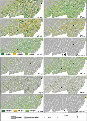
The spatial distributions of change trajectories (Figure 6) clearly shows the conversions from PF to AP in 1991–2000, from SF to AP in 2000–2008, and from AP to SF in 2008–2017. In particular, the changes from AP to SF in 2008–2011 and 2014–2017 were especially obvious. More detailed gain and loss of major land covers can be found in (Figure 7). With the longer detection interval, deforestation of PF was mainly due to conversions to SF and AP, and more PF was converted to AP than to SF before 2008 (Figure 7a). After 2008, especially in 2008–2011 and 2014–2017, more PF was converted to SF than to AP. Urban expansion after 2000 was obvious, especially in 2011–2014 at the cost of AP (Figure 7b). SF gain and loss were similar in 2000–2008, but SF gain was considerably higher in 1991–2000. Although SF gain was much higher than SF loss in 2008–2017, the gain mainly occurred in 2014–2017 at the cost of AP (Figure 7c). Previous research showed that in the 1990s much PF was converted to pasture, while from 2000 on, especially in recent years, cocoa expansion occurred in the areas of pasture (Calvi, Augusto, and Araújo 2010). As shown in (Figure 7d), AP losses were mainly due to the conversion from AP to SF, that is, from pasture to cocoa plantations.

Figure 6. Land-cover change trajectories at different detection periods (nine-year and three-year intervals) (Note: PF, primary forest; SF, secondary forest; AP, agropasture; UR, urban city; WA, water).

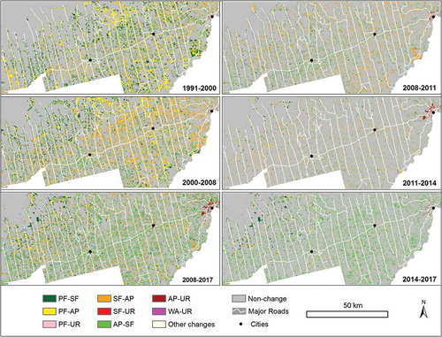
Figure 7. Comparison of land-cover changes at different detection periods (a: primary forest loss; b: urban gain; c: secondary forest loss and gain; d: agropasture loss and gain) (Note: PF, primary forest; SF, secondary forest; AP, agropasture; UR, urban; WA, water).

Different time period lengths affected change detection results. For example, the nine-year change results between 2008 and 2017 in (Figure 6) showed that major changes occurred between AP and SF, following the conversion from PF to AP and SF. The three-year change results showed large changes from SF to AP, following AP to SF between 2008 and 2011; relatively small, dispersed changes occurred between SF and AP between 2011 and 2014; and, similar to the nine-year results, large changes between 2014 and 2017 were the conversions from AP to SF, following PF to SF and AP. (Figure 8) shows that in terms of short detection intervals, PF deforestation was the most profound, and a large portion was converted to SF in 2008–2011. SF lost the most in 2008–2011 but gained the most in 2014–2017. In contrast, AP lost the most in 2014–2017 after gaining the most in 2008–2011. The greatest urban expansion happened in 2011–2014, mostly from AP, suggesting the encroachment of urban expansion at the expense of the agropasture areas in the periphery of the city with the Belo Monte dam construction beginning in 2011. By 2014, the peak of population growth had been reached, and a significant decline in population started as workers were dismissed and commercial activities declined, to an extent.

Figure 8. Individual land-cover changes over time (a: nine-year detection interval; b: three-year detection interval) (Note: PF, primary forest; SF, secondary forest; AP, agropasture; UR, urban; WA, water).

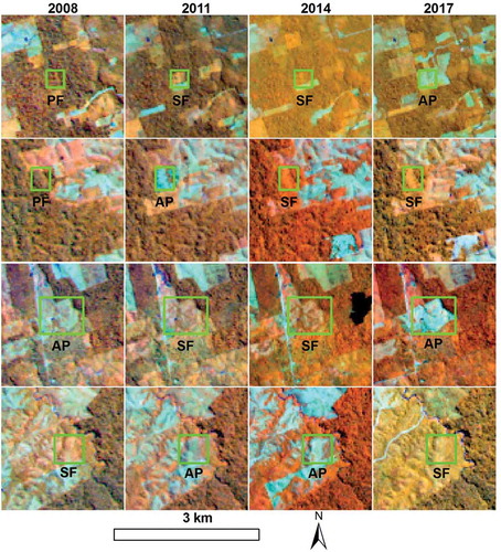
The areas of land-cover conversions between 2008 and 2017 did not match the total areas calculated from corresponding changes within shorter intervals (shaded numbers in (Table 4)), indicating that the longer period (9 years) cannot reflect the intermediate changes that occurred between 2008 and 2017 (three-year intervals). In particular, the total changed areas from SF to AP or from AP to SF based on three-year detection intervals had much higher amounts than based on a nine-year detection interval, implying that the intermediate changes between SF and AP within the detection periods were not captured within a single nine-year interval. These intermediate changes are clearly illustrated in (Figure 9). For example, PF might be cleared for AP first, then abandoned and evolve into SF in later years, or some of those new SF areas might be cleared again for cultivation after a brief fallow period. Such intermediate changes could not be identified within a long time period but could be detected within a short time period. In addition, due to back-and-forth conversions between some land-cover types, such as AP–SF–SF–AP and SF–AP–AP–SF during the periods 2008–2011–2014–2017, those kinds of changes were falsely detected as unchanged within a long time interval. Therefore, selection of a suitable time interval is critical for accurate detection of land-cover changes.

Table 4. Land-cover change trajectories over the study region at different detection periods.

Land-cover change trajectory		Changed area (ha) at nine-year intervals			Changed area (ha) at three–year intervals			Total (2008–2017)
		1991–2000	2000–2008	2008–2017	2008–2011	2011–2014	2014–2017
PF loss	PF–SF	45,513	36,096	35,271	14,208	5,940	10,638	30,786
	PF–AP	50,508	42,296	17,694	9,087	6,312	6,975	22,374
	PF–UR/WA	405	1,480	747	237	111	243	591
	Total	96,426	79,880	53,649	23,535	12,360	17,853	53,748
SF loss	SF–AP	32,463	61,408	37,458	34,686	17,988	3,684	56,358
	SF–UR/WA	279	944	738	141	264	183	588
	Total loss	32,742	62,352	38,196	34,827	18,252	3,867	56,946
SF gain	PF–SF	45,513	36,096	35,217	14,208	5,940	10,638	30,786
	AP–SF	24,057	28,408	70,893	22,851	11,796	59,409	94,056
	WA–SF	63	16	9	0	15	3	18
	Total gain	69,633	64,528	106,119	37,059	17,748	70,047	124,854
AP loss	AP–SF	24,057	28,408	70,893	22,851	11,796	59,409	94,056
	AP–UR/WA	1134	3192	4077	1,374	1638	1,560	4,572
	Total loss	25,191	31,608	74,961	24,225	13,434	60,969	98,628
AP gain	PF–AP	50,508	42,296	17,694	9,087	6,312	6,975	22,374
	SF–AP	32,463	61,408	37,458	34,686	17,988	3,684	56,358
	WA–AP	135	104	36	9	87	3	99
	Total gain	83,106	103,808	55,179	43,782	24,390	10,665	78,837
UR gain	PF–UR	207	528	423	114	63	159	336
	SF–UR	252	776	648	141	255	51	447
	AP–UR	972	2,768	3,447	1,371	1,638	900	3,909
	WA–UR	9	8	306	36	132	9	177
	Total gain	1,431	4,072	4,824	1,662	2,088	1,119	4,869
UR loss	UR–WA	0	0	36	0	0	75	75
Others		540	96	18	0	114	15	129

Note: PF, primary forest; SF, secondary forest; AP, agropasture; UR, urban; WA, water

Figure 9. Intermediate land-cover dynamic changes detected within three-year intervals between 2008 and 2017 (Note: PF, primary forest; SF, secondary forest; AP, agropasture).

4.2 Analysis of human-induced factors on deforestation and agropasture dynamics

Deforestation and AP expansion are related linearly or nonlinearly to population, GDP, and number of cattle as illustrated in (Figure 10). UR area and GDP strongly and nonlinearly relate to PF area

Figure 10. Impacts of population, economic growth, and cattle on major land-cover changes (a: impacts of urbanization on deforestation and agropasture expansion; b: impact of cattle herds on agropasture area; c: impacts of population on deforestation and agropasture expansion; d: impacts of gross domestic product on deforestation and agropasture expansion) (Note: PF, primary forest; AP, agropasture; UR, urban; GDP, gross domestic product).

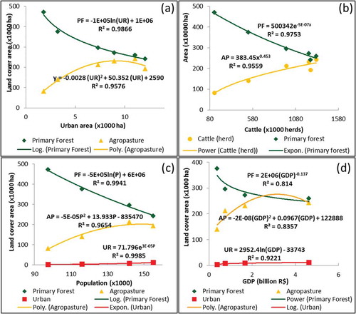
(Figure 10a,d), while number of cattle and population almost linearly relate to PF (Figure 10b,c). UR area, number of cattle, population, and GDP were positively and nonlinearly related to AP area (Figure 10a–d), while population and GDP were almost linearly related to UR area (Figure 10c,d). These relationships imply that population growth and economic conditions are important factors causing deforestation and AP expansion. The nonlinear relationships of AP area with population, GDP, and UR area may be associated with the construction of the Belo Monte dam between 2011 and 2015, as the sharp growth of population and GDP resulted in a high urbanization rate at the cost of AP conversion. This implies that an important event such as a large dam may considerably affect the land-cover change trajectories and rates; for example, by drawing farm labor to urban and dam construction.

5. Discussion

5.1. Determination of suitable temporal resolution for land-cover change detection

Much change detection research has focused on the identification of suitable remote sensing variables and detection techniques without careful consideration of temporal periods (Lu, Li, and Moran 2014). In reality, selection of suitable temporal resolution is critical for successfully detecting land-cover changes (Lu et al. 2004c; Briassoulis 2009). A long detection interval may provide general change trends over a long term, but cannot detect the intermediate change process, especially for frequently changed land covers such as AP and SF in this study. In Brazil, the common practice of deforestation is people clearing trees for cattle ranching and crop farming by logging and burning. However, the soil is rapidly degraded due to high temperatures and precipitation, and they may not be productive for farming and ranching within a few years due to improper management (Lu et al. 2004a, 2007). Thus, many lands are abandoned and convert to SF. After a couple years of soil recovery, these lands may be put back into production or AP. This requires us to carefully select temporal resolution to accurately capture the short-term land-cover change. Because cocoa has higher economic value than pasture or cropland, there was a large conversion from AP to cocoa in recent years, and we had to capture this change in the short time intervals.

Many factors such as the availability of remotely sensed data, detection contents, characteristics of the study area, and time and labor involved in the detection work may affect this determination (Lu, Li, and Moran 2014). Some important events such as natural disasters and human-induced activities like selective logging require short-term change detection intervals too. In this research, the El Niño problem in 2015/2016 may have affected land-cover change across a large area. The Belo Monte dam greatly affected the urban expansion of Altamira (Feng et al. 2017) and other land-cover changes near the dam construction area. The political and economic conditions can also indirectly affect land-cover changes, requiring change detection to be conducted in a timely way.

Although this study indicates that a three-year interval provided more land-cover change information than a nine-year interval, we cannot say this is the optimal time period because of the difficulty in collecting a sufficient number of images. In recent years, dense time-series Landsat images have been extensively applied to land-cover change detection, especially to determine forest disturbances (Huang et al. 2010; Kennedy, Yang, and Cohen 2010; Zhu and Woodcock 2014; Hermosilla et al. 2016). However, land-cover change detection in the Brazilian Amazon basin has been difficult due to cloud cover (Asner 2001), especially before 2000, when few sensor data besides Landsat 5 and SPOT images were available. Although space-based radar data such as Radarsat C-band and ALOS PALSAR L-band are available, the poor separability in land-cover classes (Li et al. 2012), especially different forest types, makes them less successful for land-cover change detection. In recent years, more sensor data such as Sentinel-2 and Landsat 8 Operational Land Imager are available at no cost, and the application of Google Earth Engine technology provides a new platform for detecting detailed land-cover change for short periods.

5.2. Forces driving land-cover change in the study region

The forces driving land-cover change have long been explored (Lambin 1997), but they vary depending on the study areas, research scales (local or regional), and data availability. It is necessary to understand the forces driving deforestation, urbanization, and AP expansion in the TransAmazon region. Previous research shows that population and economic conditions play important roles in urban expansion, and their influences are dependent upon the region and time (Kuang et al. 2014). For example, annual GDP growth per capita drove approximately half of observed urban land expansion in China, whereas urban population growth played a bigger role in India and Africa (Seto 2011). Population growth increases the demand for housing, supporting services, and facilities, resulting in urban expansion by converting vegetation and agricultural land to residential use, social and health care facilities, and infrastructure. This research also found population and economic growth were strongly related to deforestation and AP expansion. The growth of population increases the demand for food supply, thus requiring more AP lands for food and meat products, leading to AP expansion at the cost of PF deforestation. In addition to population growth, economic development creates demands for more housing space, more goods and services, better education and medical facilities, and improved infrastructure, thus accelerating urban development. Economic development also drives deforestation of PF and AP expansion. Conversion of forest to AP for cattle ranching and agriculture is the most common route to achieving economic development in the Brazilian context (Rodrigues et al. 2009). The strong relationship between number of cattle and AP area over time was indirectly conformed in Jusys (2016) that cattle ranching had the strongest impact on deforestation across the Brazilian Amazon. Jusys (2016) also established that strong relationships between GDP and urban growth and deforestation meant that high income was an accelerant of deforestation. Roads and highways have been regarded as an important factor resulting in deforestation (Soares-Filho et al. 2004), and this research showed that deforestation occurred along the roads in the early years.

The most rapid urban growth in our study area occurred during 2011–2014, coinciding with the construction of Belo Monte Dam. During this period, an estimated 20,000 people were relocated to Altamira after being removed from areas that would be flooded by the dam. At the same time, construction of the dam attracted a large number of migrant workers and service providers to Altamira. Tremendous population growth in Altamira stimulated great urban expansion (Feng et al. 2017), and thus large areas of AP lands were converted to residential use. The nonlinear relationships of AP with UR, population, and GDP (Figure 10) can be attributed to the dam construction.

Our analyses found that SF area increased dramatically after 2014 and can be partially attributed to cocoa expansion. Brazil is one of the largest cocoa-producing countries, but its production cannot meet even its own consumption and it has to import cocoa from others (Zugaib and Barreto 2015). Of the states in Brazil, Pará is the second-largest cocoa producer (Calvi, Augusto, and Araújo 2010). Recent government incentives promoting cocoa production have been extended to northern regions, like Pará, to stimulate its expansion. Cocoa plantations were grouped into SF because of their spectral similarity, and the cocoa samples collected in the field were actually located in areas classified as SF from remote sensing images.

6. Conclusions

This research examined land-cover dynamic change, especially deforestation and AP dynamics, in the TransAmazon region in the northern Brazilian state of Pará using multitemporal Landsat imagery. We examined the impacts of human-induced factors such as population growth, economic condition, and cattle raising on deforestation and AP expansion. Our research confirmed that the hierarchical-based approach can successfully classify the Landsat multispectral imagery into five land covers: PF, SF, AP, UR, and WA with an overall classification accuracy of 83.4%. PF linearly decreased from 1991 to 2017, and AP linearly increased from 1991 to 2014, but sharply decreased from 2014 to 2017. SF increased slightly from 1991 to 2000, remained stable between 2000 and 2014, then sharply increased from 2014 to 2017. UR increased linearly although it accounted for a very small proportion of change in this study area. Deforestation of PF accounted for a large proportion of the land-cover change, especially before 2000, but the dynamic changes between SF and AP became more important in the last decade. This research indicates that a time interval of 9 years cannot effectively detect the dynamic changes between SF and AP and needs to be shorter, implying the necessity to identify suitable temporal resolution in land-cover change detection. In addition to the common factors – population and economic conditions – affecting land-cover change, this research indicates that number of cattle and policies to expand cocoa plantations also affect deforestation and the dynamic changes between SF and AP. Population growth associated with the construction of the dam led to urban expansion at the expense of AP. The Belo Monte dam construction was an important factor resulting in AP and SF dynamic changes.

Acknowledgements

This work was supported by the Fundação de Amparo a Pesquisa do Estado de São Paulo (processo 2012/51465-0), under the São Paulo Excellence Chairs Program, awarded to Emilio F. Moran as PI; US National Science Foundation under grant 1639115 to Moran as PI; Michigan State University through research funds provided to Dengsheng Lu and Emilio F. Moran. Luciano Vieira Dutra and Miquéias Freitas Calvi thank the Conselho Nacional de Desenvolvimento Científico e Tecnológico for supporting fieldwork through grants #401528/2012-0, #309135/2015-0, and #409936 2013-8.

Disclosure statement

No potential conflict of interest was reported by the authors.

Additional information

Funding

This work was supported by the Fundação de Amparo à Pesquisa do Estado de São Paulo [2012/51465-0];National Science Foundation [1639115];Zhejiang Agriculture and Forestry University’s Research and Development Fund [2013FR052];

References

- Asner, G. P. 2001. “Cloud Cover in Landsat Observations of the Brazilian Amazon.” International of Remote Sensing 22 (18): 3855–3862. doi:10.1080/01431160010006926.
- Atkins, E. 2017. “Dammed and Diversionary: The Multi-Dimensional Framing of Brazil’s Belo Monte Dam.” Singapore Journal of Tropical Geography 38 (3): 276–292. doi:10.1111/sjtg.12206.
- Beuchle, R., R. C. Grecchi, Y. E. Shimabukuro, R. Seliger, H. D. Eva, E. Sano, and F. Achard. 2015. “Land Cover Changes in the Brazilian Cerrado and Caatinga Biomes from 1990 to 2010 Based on a Systematic Remote Sensing Sampling Approach.” Applied Geography 58: 116–127. doi:10.1016/j.apgeog.2015.01.017.
- Briassoulis, H. 2009. “Factors Influencing Land-Use and Land-Cover Change.” In: Encyclopedia of Land Use, Land Cover and Soil Sciences: Land Cover, Land Use and Global Change, edited by W. H. Verhey. Encyclopedia of Life Support Systems (EOLSS) I:125–145. Oxford: Eolss Publishers. URL https://www.eolss.net/TOC/C19-BrowseContents.aspx (membership required).
- Brondízio, E. S. 2005. “Intraregional Analysis of Land-Use Change in the Amazon.” In Seeing the Forest and the Trees: Human-Environment Interactions in Forest Ecosystems, edited by E. F. Moran and E. Ostrom, 223–252. Cambridge: MIT.
- Calvi, M. F. 2009. “Fatores de adoção de sistemas agroflorestais por agricultores familiares do município de Medicilândia, Pará.” Belém, Brasil: Universidade Federal do Pará. URL: https://ainfo.cnptia.embrapa.br/digital/bitstream/item/45741/1/AA-MIQUEIAS-FREITAS-CALVI.pdf.
- Calvi, M. F., S. G. Augusto, and A. Araújo. 2010. Diagnóstico Do Arranjo Produtivo Local Da Cultura Do Cacau No Território Da Transamazônica – Pará. Altamira: SEBRAE/UFPA.
- Chander, G., B. L. Markham, and D. L. Helder. 2009. “Summary of Current Radiometric Calibration Coefficients for Landsat MSS, TM, ETM+, and EO-1 ALI Sensors.” Remote Sensing of Environment 113 (5): 893–903. doi:10.1016/j.rse.2009.01.007.
- Chávez, P. S. Jr. 1996. “Image-Based Atmospheric Corrections – Revisited and Improved.” Photogrammetric Engineering and Remote Sensing 62 (9): 1025–1036. 0099-1112/96/6209-1025.
- Chen, G., R. P. Powers, L. M. T. De Carvalho, and B. Mora. 2015. “Spatiotemporal Patterns of Tropical Deforestation and Forest Degradation in Response to the Operation of the Tucuruí Hydroelectric Dam in the Amazon Basin.” Applied Geography 63: 1–8. doi:10.1016/j.apgeog.2015.06.001.
- Congalton, R. G., and K. Green. 2009. Assessing the Accuracy of Remotely Sensed Data: Principles and Practices. Boca Raton: CRC Press/Taylor & Francis.
- Fearnside, P. M. 2016. “Environmental and Social Impacts of Hydroelectric Dams in Brazilian Amazonia: Implications for the Aluminum Industry.” World Development 77: 48–65. doi:10.1016/J.WORLDDEV.2015.08.015.
- Feng, Y., D. Lu, E. F. Moran, L. V. Dutra, M. F. Calvi, and M. A. F. Oliveira. 2017. “Examining Spatial Distribution and Dynamic Change of Urban Land Covers in the Brazilian Amazon Using Multitemporal Multisensor High Spatial Resolution Satellite Imagery.” Remote Sensing 9 (4): 381. doi:10.3390/rs9040381.
- Foody, G. M. 2002. “Status of Land Cover Classification Accuracy Assessment.” Remote Sensing of Environment 80 (1): 185–201. doi:10.1016/S0034-4257(01)00295-4.
- Government, B. 2017. Investment Guide to Brasil 2017. URL: https://investexportbrasil.dpr.gov.br/Arquivos/Publicacoes/Estudos/InvestmentGuide2017.pdf.
- Grecchi, R. C., R. Beuchle, Y. E. Shimabukuro, L. E. O. C. Aragão, E. Arai, D. Simonetti, and F. Achard. 2017. “An Integrated Remote Sensing and GIS Approach for Monitoring Areas Affected by Selective Logging: A Case Study in Northern Mato Grosso, Brazilian Amazon.” International Journal of Applied Earth Observation and Geoinformation 61: 70–80. doi:10.1016/j.jag.2017.05.001.
- Grecchi, R. C., Q. H. J. Gwyn, G. B. Bénié, A. R. Formaggio, and F. C. Fahl. 2014. “Land Use and Land Cover Changes in the Brazilian Cerrado: A Multidisciplinary Approach to Assess the Impacts of Agricultural Expansion.” Applied Geography 55: 300–312. doi:10.1016/j.apgeog.2014.09.014.
- Hermosilla, T., M. A. Wulder, J. C. White, N. C. Coops, G. W. Hobart, and L. B. Campbell. 2016. “Mass Data Processing of Time Series Landsat Imagery: Pixels to Data Products for Forest Monitoring.” International Journal of Digital Earth 9 (11): 1035–1054. doi:10.1080/17538947.2016.1187673.
- Huang, C., S. N. Goward, J. G. Masek, N. Thomas, Z. Zhu, and J. E. Vogelmann. 2010. ““An Automated Approach for Reconstructing Recent Forest Disturbance History Using Dense Landsat Time Series Stacks.” Remote Sensing of Environment 114 (1): 183–198. doi:10.1016/j.rse.2009.08.017.
- Imbach, P., M. Manrow, E. Barona, A. Barretto, G. Hyman, and P. Ciais. 2015. “Spatial and Temporal Contrasts in the Distribution of Crops and Pastures across Amazonia: A New Agricultural Land Use Data Set from Census Data since 1950.” Global Biogeochemical Cycles 29 (6): 898–916. doi:10.1002/2014GB004999.
- Jusys, T. 2016. “Fundamental Causes and Spatial Heterogeneity of Deforestation in Legal Amazon.” Applied Geography 75: 188–199. doi:10.1016/j.apgeog.2016.08.015.
- Karathanassi, V., P. Kolokousis, and S. Ioannidou. 2007. “A Comparison Study on Fusion Methods Using Evaluation Indicators.” International Journal of Remote Sensing 28 (10): 2309–2341. doi:10.1080/01431160600606890.
- Kennedy, R. E., Z. Q. Yang, and W. B. Cohen. 2010. “Detecting Trends in Forest Disturbance and Recovery Using Yearly Landsat Time Series: 1. LandTrendr - Temporal Segmentation Algorithms.” Remote Sensing of Environment 114 (12): 2897–2910. doi:10.1016/j.rse.2010.07.008.
- Kuang, W., W. Chi, D. Lu, and Y. Dou. 2014. “A Comparative Analysis of Megacity Expansions in China and the U.S.: Patterns, Rates and Driving Forces.” Landscape and Urban Planning 132: 121–135. doi:10.1016/j.landurbplan.2014.08.015.
- Lambin, E. F. 1997. “Modelling and Monitoring Land-Cover Change Processes in Tropical Regions.” Progress in Physical Geography 21 (3): 375–393. doi:10.1177/030913339702100303.
- Li, G., D. Lu, E. Moran, and S. Hetrick. 2011. “Land-Cover Classification in a Moist Tropical Region of Brazil with Landsat Thematic Mapper Imagery.” International Journal of Remote Sensing 32 (23): 8207–8230. doi:10.1080/01431161.2010.532831.
- Li, G., D. Lu, E. Moran, and S. J. S. Sant’Anna. 2012. “Comparative Analysis of Classification Algorithms and Multiple Sensor Data for Land Use/Land Cover Classification in the Brazilian Amazon.” Journal of Applied Remote Sensing 6 (1): 061706. doi:10.1117/1.JRS.6.061706. Dec 14, 2012.
- Lu, D., M. Batistella, P. Mausel, and E. Moran. 2007. “Mapping and Monitoring Land Degradation Risks in the Western Brazilian Amazon Using Multitemporal Landsat TM/ETM+ Images.” Land Degradation and Development 18 (1): 41–54. doi:10.1002/ldr.762.
- Lu, D., S. Hetrick, E. Moran, and G. Li. 2010. “Detection of Urban Expansion in an Urban-Rural Landscape with Multitemporal QuickBird Images.” Journal of Applied Remote Sensing 4: 041880. doi:10.1117/1.3501124.
- Lu, D., S. Hetrick, E. Moran, and G. Li. 2012. “Application of Time Series Landsat Images to Examining Land-use/Land-Cover Dynamic Change.” Photogrammetric Engineering & Remote Sensing 78 (7): 747–755. doi:10.14358/PERS.78.7.747.
- Lu, D., G. Li, and E. Moran. 2014. “Current Situation and Needs of Change Detection Techniques.” International Journal of Image and Data Fusion 5: 13–38. doi:10.1080/19479832.2013.868372.
- Lu, D., G. Li, E. Moran, and S. Hetrick. 2013. “Spatiotemporal Analysis of Land-Use and Land-Cover Change in the Brazilian Amazon.” International Journal of Remote Sensing 34 (16): 5953–5978. doi:10.1080/01431161.2013.802825.
- Lu, D., G. Li, G. S. Valladares, and M. Batistella. 2004a. “Mapping Soil Erosion Risk in Rondônia, Brazilian Amazonia: Using Rusle, Remote Sensing and GIS.” Land Degradation & Development 15: 499–512. doi:10.1002/ldr.634.
- Lu, D., P. Mausel, M. Batistella, and E. Moran. 2004b. “Comparison of Land-Cover Classification Methods in the Brazilian Amazon Basin.” Photogrammetric Engineering & Remote Sensing 70 (6): 723–731. doi:10.14358/PERS.70.6.723.
- Lu, D., P. Mausel, E. Brondízio, and E. Moran. 2004c. “Change Detection Techniques.” International Journal of Remote Sensing 25 (12): 2365–2407. doi:10.1080/0143116031000139863.
- Moran, E. F. 1975. “The Brazilian Colonization Experience in the Transamazon Highway.” Papers in Anthropology 16 (1): 29–57.
- Moran, E. F. 1981. Developing the Amazon. Bloomington: Indiana University Press.
- Moran, E. F. 2016. “Roads and Dams: Infrastructure-Driven Transforamtions in the Brazilian Amazon.” Ambiente & Sociedade 19 (2): 207–220. doi:10.1590/1809-4422ASOC256V1922016.
- Moran, E. F., and E. Brondizio. 1998. “Land-Use Change after Deforestation in Amazonia.” In People and Pixels: Linking Remote Sensing and Social Science, edited by D. Liverman, E. F. Moran, R. R. Rindfuss, and P. Stern, 94–120. Washington, DC: National Academies Press.
- Moran, E. F., E. Brondizio, P. Mausel, and Y. Wu. 1994. “Integrating Amazonian Vegetation, Land-Use, and Satellite Data.” BioScience 44 (5): 329–338. doi:10.2307/1312383.
- Müller, H., P. Griffiths, and P. Hostert. 2016. “Long-Term Deforestation Dynamics in the Brazilian Amazon—Uncovering Historic Frontier Development along the Cuiabá–Santarém Highway.” International Journal of Applied Earth Observation and Geoinformation 44: 61–69. doi:10.1016/j.jag.2015.07.005.
- Ritter, C. D., G. McCrate, R. H. Nilsson, P. M. Fearnside, U. Palme, and A. Antonelli. 2017. “Environmental Impact Assessment in Brazilian Amazonia: Challenges and Prospects to Assess Biodiversity.” Biological Conservation 206: 161–168. doi:10.1016/j.biocon.2016.12.031.
- Rodrigues, A. S. L., R. M. Ewers, L. Parry, C. Souza, A. Veríssimo, and A. Balmford. 2009. “Boom-and-Bust Development Patterns across the Amazon Deforestation Frontier.” Science 324 (5933): 1435–1437. doi:10.1126/science.1174002.
- Schneibel, A., D. Frantz, A. Röder, M. Stellmes, K. Fischer, and J. Hill. 2017. “Using Annual Landsat Time Series for the Detection of Dry Forest Degradation Processes in South-Central Angola.” Remote Sensing 9 (9): 905. doi:10.3390/rs9090905.
- Seto, K. C. 2011. “Exploring the Dynamics of Migration to Mega-Delta Cities in Asia and Africa: Contemporary Drivers and Future Scenarios.” Global Environmental Change 21 (SUPPL. 1): 94–107. doi:10.1016/j.gloenvcha.2011.08.005.
- Shimizu, K., R. Ponce-Hernandez, O. S. Ahmed, T. Ota, Z. C. Win, N. Mizoue, and S. Yoshida. 2017. “Using Landsat Time Series Imagery to Detect Forest Disturbance in Selectively Logged Tropical Forests in Myanmar.” Canadian Journal of Forest Research 47: 289–296. doi:10.1139/cjfr-2016-0244.
- Silveira, E. M. O., J. M. Mello, F. W. Acerbi Jr, and L. M. T. Carvalho. 2018. “Object-Based Land-Cover Change Detection Applied to Brazilian Seasonal Savannahs Using Geostatistical Features.” International Journal of Remote Sensing 39 (8): 2597–2619. doi:10.1080/01431161.2018.1430397.
- Soares-Filho, B., A. Alencar, D. Nepstad, G. Cerqueira, M. D. C. Vera Diaz, S. Rivero, L. Solórzano, and E. Voll. 2004. “Simulating the Response of Land-Cover Changes to Road Paving and Governance along a Major Amazon Highway: The Santarém-Cuiabá Corridor.” Global Change Biology 10 (5): 745–764. doi:10.1111/j.1529-8817.2003.00769.x.
- Spera, S. A., A. S. Cohn, L. K. Vanwey, J. F. Mustard, B. F. Rudorff, J. Risso, and M. Adami. 2014. “Recent Cropping Frequency, Expansion, and Abandonment in Mato Grosso, Brazil Had Selective Land Characteristics.” Environmental Research Letters 9: 064010. doi:10.1088/1748-9326/9/6/064010.
- Tucker, J. M., E. S. Brondizio, and E. F. Morán. 1998. “Rates of Forest Regrowth in Eastern Amazónia: A Comparison of Altamira and Bragantina Regions, Pará State, Brazil.” Interciencia 23: 64–73.
- Tundisi, J. G., T. Matsumura-Tundisi, and J. E. Tundisi. 2015. “Environmental Impact Assessment of Reservoir Construction: New Perspectives for Restoration Economy, and Development: The Belo Monte Power Plant Case Study.” Brazilian Journal of Biology 75 (3 suppl 1): 10–15. doi:10.1590/1519-6984.03514BM.
- Walker, R., and A. K. O. Homma. 1996. “Land Use and Land Cover Dynamics in the Brazilian Amazon: An Overview.” Ecological Economics 18 (1): 67–80. doi:10.1016/0921-8009(96)00033-X.
- Walker, R., E. Moran, and L. Anselin. 2000. “Deforestation and Cattle Ranching in the Brazilian Amazon: External Capital and Household Processes.” World Development 28 (4): 683–699. doi:10.1016/S0305-750X(99)00149-7.
- Zhu, Z., and C. E. Woodcock. 2014. “Continuous Change Detection and Classification of Land Cover Using All Available Landsat Data.” Remote Sensing of Environment 144: 152–171. doi:10.1016/j.rse.2014.01.011.
- Zugaib, A. C. C., and R. C. S. Barreto. 2015. “O mercado Brasileiro de cacau: Perspectivas de demanda, oferta e preços.” Agrotrópica 27 (3): 303–316. doi:10.21757/0103-3816.2015v27n3p303-316.