Monitoring surface changes in discontinuous permafrost terrain using small baseline SAR interferometry, object-based classification, and geological features: a case study from Mayo, Yukon Territory, Canada

Abstract

Permafrost-induced deformation of ground features is threating infrastructure in northern communities. An understanding of permafrost distribution is therefore critical for sustainable adaptation planning and infrastructure maintenance. Considering the large area underlain by permafrost in the Yukon Territory, there is a need for baseline information to characterize the permafrost in this region. In this study, the Differential Interferometric Synthetic Aperture Radar (DInSAR) technique was used to identify areas of ground movement likely caused by changes in permafrost. The DInSAR technique was applied to a series of repeat-pass C-band RADARSAT-2 observations collected in 2015 over the Village of Mayo, in central Yukon Territory, Canada. The conventional DInSAR technique demonstrated that ground deformation could be detected in this area, but the resulting deformation maps contained errors due to a loss of coherence from changes in vegetation and atmospheric phase delay. To address these limitations, the Small BAseline Subset (SBAS) InSAR technique was applied to reduce phase error, thus improving the deformation maps. To understand the relationship between the deformation maps and land cover types, an object-based Random Forest classification was developed to classify the study area into different land cover types. Integration of the InSAR results and the classification map revealed that the built-up class (e.g., airport) was affected by subsidence on the order of −2 to −4 cm. The spatial extent of the surface displacement map obtained using the SBAS InSAR technique was then correlated with the surficial geology map. This revealed that much of the main infrastructure in the Village of Mayo is underlain by interbedded glaciofluvial and glaciolacustrine sediments, the latter of which caused the most damage to human made structures. This study provides a method for permafrost monitoring that builds upon the synergistic use of the SBAS InSAR technique, object-based image analysis, and surficial geology data.

Keywords:

• permafrost
• interferometric SAR
• small baseline subset
• RADARSAT-2
• random forest classification
• geology

1. Introduction

One of the most important challenges faced by northern communities is climate change. The catastrophic effects of the warming climate have been frequently reported, which highlight the significance of adaptation to climate change (Northern Climate Exchange 2011). The preliminary step for climate change adaptation is to identify vulnerabilities to mitigate or at least reduce the negative effects of current and future climate change.

Permafrost is defined as soil that has remained frozen for a minimum of two consecutive years (Van Everdingen 1998). Approximately 24% of the land surface in the northern hemisphere is affected by permafrost (Antonova et al. 2016). Climate is the most influential factor on permafrost activity and the occurrence of permafrost tends to increase with latitude. Other factors, such as hydrology, topography, surficial geology, and biology (e.g., vegetation cover) are also important. Permafrost may be overlain by an active layer that thaws and freezes seasonally (Muller 1947). Surface uplift (frost heave) caused by freezing (aggradation), and ground subsidence caused by thawing, are common due to seasonal changes in the active layer. While permafrost is a subsurface phenomenon, changes in its state affect ground surface features, and potentially engineering infrastructure (Short et al. 2011). Seasonal changes of the active layer affect engineering infrastructure to a lesser extent than the long-term degradation of the permafrost layer due to climate change. This indicates the necessity of continual monitoring of surface movement in permafrost regions for identifying potential geo-hazards associated with this phenomenon.

The remoteness, vastness, and inaccessibility of the ground affected by permafrost constrain the application of traditional approaches (e.g., surveying) for permafrost monitoring (Antonova et al. 2016). Satellite remote sensing data provide a unique source of information and mitigate the main limitations of traditional approaches. Synthetic Aperture Radar (SAR) sensors acquire data independently of solar radiation and are unaffected by cloud cover, which often prevents optical sensors from monitoring permafrost environments (Antonova et al. 2016). Backscatter intensity is one of the fundamental observations of SAR imagery and is mainly sensitive to surface roughness and the dielectric constant of surface materials (Ferretti et al. 2007). An increase in surface roughness and/or the dielectric constant increases SAR backscatter intensity. Surface roughness depends on the scale of the ground targets relative to the SAR wavelength and determines the type of scattering mechanisms, while the dielectric constant is affected by water content (soil moisture). For example, saturated soil has a large dielectric constant and a higher backscattering response in SAR images. In contrast, frozen water has a significantly lower dielectric constant relative to liquid water and, consequently, freezing and thawing statuses have low and high backscattering responses in SAR imagery, respectively (Wegmüller 1990).

To characterize and understand the influence of permafrost and changes in the active layer on the ground surface, a land cover classification map of the area is required. Such a land cover map is useful for understanding the spatial variability of displacement caused by permafrost and its relationship with various land cover classes (e.g., vegetation, bare land, and built-up).

The Differential Interferometric SAR (DInSAR) technique is an efficient tool for measuring ground deformation induced by volcanos, earthquakes, and landslides (Ferretti et al. 2007). It has also shown good results for monitoring ground subsidence in several recent studies (Dehghan-Soraki, Sharifikia, and Sahebi 2015; Zhou et al. 2016; Chen et al. 2017; Deng et al. 2017; Fiaschi et al. 2017; Suresh Krishnan, Kim, and Jung 2018). Importantly, the DInSAR technique is useful for mapping deformation due to permafrost activity, since deformation occurs at the ground surface (Short et al. 2011). Short et al. (2011) reported the potential of the DInSAR technique for measuring deformation caused by permafrost on Herschel Island located off the northern Yukon coast using three SAR frequencies (i.e., L-, C-, and X-band). However, the main limitations of the conventional DInSAR technique are temporal and spatial decorrelation, as well as atmospheric disturbances (Chen et al. 2012). Advanced InSAR time series techniques, such as persistent scatterer interferometry (PSI) (Ferretti, Prati, and Rocca 2000) and small baseline subset interferometry (SBAS) (Berardino et al. 2002), show great promise for reducing these errors. These advanced InSAR methods combine a stack of differential SAR interferograms, allowing the temporal evolution of the deformation signal to be retrieved. The applications of advanced InSAR techniques for measuring permafrost-induced deformation have been previously investigated in some studies (Chen et al. 2013; Zhao et al. 2016; Antonova et al. 2016).

Interferometric coherence shows the quality of interferometric processing by measuring the degree of similarity between two pixels with the same location during the time interval of two SAR acquisitions (Ferretti et al. 2007). Coherence is defined using both the amplitude and phase of the SAR signal and, as such, is more sensitive to ground changes relative to backscatter intensity (i.e., amplitude alone; Ramsey et al., 2006). Some studies have reported that coherence augments intensity observations by offering additional information (Strozzi, Wegmuller, and Matzler 1999; Ramsey et al., 2006; Mohammadimanesh et al. 2018a, 2018b). However, the application of interferometric coherence for land cover mapping remains underrepresented and has only been investigated in a few studies of change detection in glacier surfaces (Weydahl 2001), Arctic classification (Hall-Atkinson and Smith 2001), and mapping wet snow coverage (Strozzi, Wegmuller, and Matzler 1999).

Despite recent research into the use of the InSAR technique for permafrost monitoring within the continuous permafrost zone (Short et al. 2011, 2014; Rudy et al. 2018), its capability in the discontinuous permafrost zone has been underinvestigated. Permafrost within the discontinuous zone is characterized by a heterogeneous landscape, various patches of frozen ground, a deeper active layer, and more expansive vegetation cover (e.g., trees and large shrubs; Wolfe et al. 2014), all of which impose challenges to the application of the InSAR technique. Accordingly, the main objective of this study was to determine the magnitude and pattern of displacement caused by permafrost using the InSAR technique in the Mayo area, Yukon Territory, located within the extensive discontinuous permafrost region. An object-based Random Forest rule-set was also developed for land cover classification using SAR and optical imagery. Furthermore, all available ancillary data, such as a surficial geology map, were also used to determine the relationship between movements identified by InSAR and the geological units. Specifically, the correlation between the displacement results, surficial geology units, and land-cover classification map was determined to understand and characterize the pattern and magnitude of displacement in various land cover and surface geology types. This allowed us to interpret seasonal changes within the permafrost regions caused by climatic, geologic, and land cover factors. To the best of our knowledge, this is the first to determine the distribution of permafrost-affected areas using these remote sensing tools and data in the Village of Mayo. Knowledge of the distribution of permafrost, changes (e.g., degradation) to the existing permafrost regime, and subsequent ground motion are important to determine strategies for infrastructure maintenance.

2. Study area

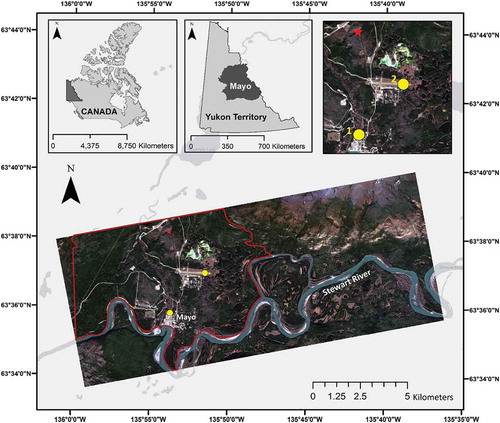
The study area is located in the central Yukon Territory (63${ }^{\circ }$ 37$\prime$ N, 135${ }^{\circ }$ 52$\prime$ W) within the Stewart River Plateau, in the community of Mayo (Figure 1). It has a population of 200 people and there were 100 occupied private dwellings as per the 2016¹ Census.

Figure 1. True colour composite (bands 4, 3, and 2) of Sentinel-2 imagery, acquired on 6 October 2016, representing the geographic location of the study area. Note that the yellow points are the locations of field investigations in the summer of 2010 by the Northern Climate Exchange (2011). Points 1 and 2 are located at the J. V. Clark School and the Mayo Airport, respectively. The red star represents the location of the InSAR reference point and the red polygon shows the extent of the surficial geology map (Kennedy 2011).

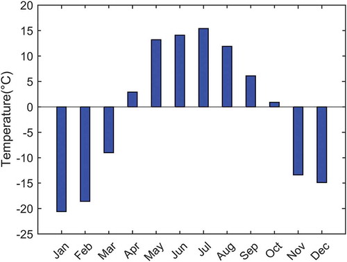
The Mayo region has a subarctic continental climate, experiencing short, relatively warm summers, and long, cold winters (Smith, Miekle, and Roots 2004). Mean annual temperatures in this region range from −27${ }^{\circ }$C in January to 15.5${ }^{\circ }$C in July, based on 26 years (1964–1990) of climate measurements. However, the mean annual temperature has increased with a rate of 0.3${ }^{\circ }$C per decade in the period between 1979 and 2009. Figure 2 represents the average temperature for each month in 2015. The main source of moisture is the Pacific Ocean (Smith, Miekle, and Roots 2004) and the average annual precipitation is 318.4 mm, one third of which falls as snow (Northern Climate Exchange 2011).

Figure 2. The average temperature for each month in 2015 in the Mayo region (http://climate.weather.gc.ca/climate_data/).

The dominant vegetation type is the northern mixed deciduous and coniferous forest (Boreal forest), containing predominantly white spruce (Picea glauca) with minor amounts of black spruce (Picea mariana) and paper birch (Betula papyrifera). Aspen (Populus tremuloides), balsam (Populus balsamifera), and poplar (Populous) are also common. Artemesia grasslands or steppe vegetation are found in south-facing slopes (Northern Climate Exchange 2011).

Surficial geology in this region is dominated by a glaciated landscape that has been affected by significant modification by fluvial, eolian, and permafrost processes. The Village of Mayo is located within the area where the highest extent of the last glaciation occurred in Yukon, known as the McConnell Glaciation. As the glacier retreated, deglacial lakes and deltas filled the valley and left thick deposits of fine-grained lacustrine and coarse-grained glaciofluvial materials (Northern Climate Exchange 2011; Kennedy 2011).

The permafrost thickness varies widely and can be as thin as 5–7 m or as thick as 30–40 m within the Village of Mayo; however, the field survey has shown that thin permafrost was dominant (Northern Climate Exchange 2011). This thin permafrost is potentially relatively warm and thus is thaw sensitive. The thickness of the active layer was found to vary between 65 cm and 1 m near Mayo. The frozen ground temperature is presumably between −0.5${ }^{\circ }$C and 0${ }^{\circ }$C, suggesting the high sensitivity of the permafrost to climate warming (Hennessey, Stuart, and Duerden 2012).

Topography, vegetation cover, and snow depth during winter influence the permafrost in this region (Hennessey, Stuart, and Duerden 2012). Mayo lies in the extensive discontinuous permafrost zone according to the Permafrost Map of Canada (50–90%) (Heginbottom, Dubreuil, and Harker 1995; Burn 2000). In such a permafrost zone, there are regions where the average ground temperature is less than 0${ }^{\circ }\mathrm{C}$ (permafrost regions), and other nearby areas where the average ground temperature is greater than 0${ }^{\circ }\mathrm{C}$ (non-permafrost regions). There is a high potential for thawing of permafrost when the ground temperatures approach 0${ }^{\circ }\mathrm{C}$(Northern Climate Exchange 2011; Throop, Lewkowicz, and Smith 2012)$.$This is often observed in relation to disturbances of the natural overlaying materials caused by the removal of vegetation, forest fires, as well as climate change.

3. Dataset

Various types of Earth Observation (EO) data including SAR and optical, as well as ancillary data were used in this work. EO data included RADARSAT-2 and Sentinel-2, and ancillary data consisted of a Digital Elevation Model (DEM), surficial geology, and hazard maps. A total of 12 C-band Single Look Complex (SLC) RADARSAT-2 images with horizontal transmit and horizontal receive (HH) polarization, acquired during the interval between March and December 2015, were used for InSAR processing. This imagery was acquired using the Spotlight beam mode (SLA10) from the ascending orbit with a resolution of approximately 2.6 m and incidence angle of 38${ }^{\circ }$. For land cover classification, both RADARSAT-2 and Sentinel-2 data were used. Sentinel-2 imagery, acquired on October, 6, 2016, has 13 spectral bands in the visible, NIR, and SWIR region of the electromagnetic spectrum. A 30 m resolution DEM (http://geogratis.gc.ca/) was used for topographic phase removal during InSAR processing. In addition, a Mayo surficial geology map (Kennedy 2011) and a hazard map (http://data.geology.gov.yk.ca/Reference/50309) were used for the interpretation of the results obtained from both InSAR processing and classification.

Training and testing data for the purpose of supervised classification and accuracy assessment, respectively, were collected using visual analysis of Google Earth imagery, ancillary data, including a surficial geology and a vegetation inventory map (Energy Mines and Resources – Yukon Government), and aerial (Energy Mines and Resources – Yukon Government) and satellite imagery. Using these data and previous studies carried out in this area (Burn and Friele 1989; Burn 2000; Karunaratne and Burn 2004; Bleiler, Burn, and O’Donoghue 2006; Northern Climate Exchange 2011; Hennessey, Stuart, and Duerden 2012), auxiliary information was extracted and used to produce reference polygons representing five major classes, including forest, sparse vegetation, built-up, bare land, and water. These polygons were then sorted by size and alternatively assigned to the training (~50%) and testing polygons (~50%). This alternative assignment ensured that both the training and testing samples had comparable pixel counts for each class, resulting in a robust classification accuracy assessment. Figure 3 displays the distribution of the training and the testing polygons for each land cover type across the study area.

Figure 3. Distribution of reference data (A) training and (B) testing polygons used for object-based classification.

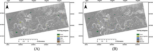
Table 1 presents the number of pixels used for training the classifier and assessing the classification result for each class. As shown, the forest and sparse vegetation classes have the most associated pixels, whereas the built-up and bare land classes have the least. This is because some land cover classes are easily identifiable via satellite imagery (e.g., forest) and are often more expansive relative to other land cover classes (e.g., bare land). Accordingly, there is a variation in the quantity and quality of reference data for each class.

Table 1. A description of the land cover classes with training and testing pixel counts.

Class	Class description	#Training pixels	#Testing pixels	Total
Forest	Boreal forest.	79,531	82,223	161,754
Sparse vegetation	Sparse vegetation, including grasslands or steppe vegetation.	41,235	40,570	81,805
Built-up	Human made structures, including airstrip, buildings, and roads.	12,871	11,448	24,319
Water	Rivers and small lakes.	28,565	29,135	57,700
Bare land	Lands not containing human made structures and vegetation.	15,682	15,061	30,743
Total		177,884 (~50%)	178,437 (~50%)	356,321

4. Methods

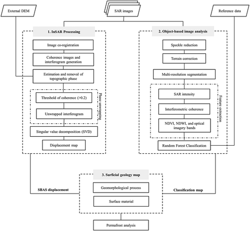
The methodology used in this study consisted of the three major steps outlined in Figure 4 and described in detail in the following sections. In the first step, repeat-pass RADARSAT-2 images were processed using the conventional DInSAR technique and later improved using the SBAS InSAR technique. The main products of the first step were the coherence images and the SBAS InSAR displacement map. The coherence images were applied to Step 2, the object-based image analysis, whereas the displacement map was used in Step 3 for the final permafrost analysis. In Step 2, following image pre-processing, including speckle reduction and terrain correction (Mahdianpari, Salehi, and Mohammadimanesh 2017a), a multi-resolution segmentation was carried out. Next, several SAR and optical features were extracted and used as input features for classification. This step produced a classification map with five main land cover classes, namely forest, sparse vegetation, water, built-up, and bare land classes. Surficial geology features, such as geomorphological processes and surface materials, are influential factors that were taken into account for permafrost analysis. The relationships between the SBAS InSAR displacement map (Step 1), the land cover classification map (Step 2), and surficial geology features were investigated in the last step (Step 3).

Figure 4. Flowchart of the methodology used in this study.

4.1. InSAR processing (step 1)

All interferometric processing was carried out using the GAMMA Remote Sensing software package. The conventional DInSAR method was used to obtain deformation maps. The conventional DInSAR processing chain begins by considering one SAR image as the master image, which is used as a reference to resample the secondary (slave) SAR image(s) into the master’s geometry. The general processing chain in conventional DInSAR includes image co-registration, coherence calculation, interferogram generation, orbital correction, estimation and removal of the topographic phase using an external DEM, differential interferogram generation, phase unwrapping, and production of unwrapped differential interferograms. The InSAR deformation results were generated relative to the point indicated by the red star in Figure 1. This point was not vegetated and consistently demonstrated high coherence and, thus, was considered to be stable.

Repeat-pass SAR data are useful for InSAR processing whenever the interferometric coherence is relatively high among the SAR images. Coherence determines the degree of similarity between two SAR images and can be affected by vegetation change, human activity, and changes in soil moisture (Mohammadimanesh et al. 2018c). Coherence values range between 0, indicating total decorrelation, and 1, representing a perfect correlation between the phase at a particular point in both the master and slave images. Generally, deformation values can be generated using the DInSAR technique for coherence values above 0.2 (Ferretti et al. 2007). In this study, the coherence threshold of 0.2 was therefore selected to avoid error during phase unwrapping (i.e., phase jump) and to eliminate pixels affected by high phase noise (Chu and Lindenschmidt 2017).

In addition to temporal and spatial decorrelation, other factors affect the quality of the DInSAR deformation results such as DEM and phase unwrapping errors (Ferretti et al. 2007). To address these limitations, the SBAS InSAR technique, proposed by Berardino et al. (2002), was pursued. This technique is suitable for a natural environment consisting of distributed scatterers and can be used to improve the ground movement results obtained from the conventional DInSAR technique. The SBAS InSAR technique determines the temporal evolution of the deformation signal by producing interferograms with a small spatial baseline to decrease the spatial decorrelation effect (Berardino et al. 2002). In this configuration, more than one interferogram has information from each SAR image when the input data are properly linked together without temporal gaps. The algorithm assumes that the deformation phase at time $n$ can be expressed as a linear combination of the connected measurements in the input data. The SBAS InSAR technique uses singular value decomposition (SVD) to combine independently unwrapped interferograms to produce a time-series. Topographic, atmospheric, and deformation signals are included in the unwrapped, co-registered interferograms. The topographic residual phase is then removed using a least squares analysis on the stack of unwrapped interferograms and a second unwrapping step is applied to the residual phase component. Atmospheric phase artifacts are also identified and removed by filtering, as they are characterized by high spatial and low temporal correlation (Berardino et al. 2002). Finally, the SBAS InSAR displacement in radians (LOS) is converted to vertical displacement using the following equation (Short et al. 2014):

(1) $d_v=\frac{\phi \left(\lambda /4\pi \right)}{cos\theta }$(1)

where $d_v$ is vertical displacement, $\phi$ is the unwrapped differential phase in radians, $\lambda$ is the SAR wavelength, and $\theta$ is the SAR incidence angle (38${ }^{\circ }$ for RADARSAT-2 SLA10 mode). Notably, vertical displacement was considered to be generally appropriate for the relatively low-relief Mayo areas where topography does not change considerably. Figure 5 demonstrates the SBAS network for the time-series analysis in this study.

Figure 5. The SBAS network for time-series analysis. A total of 12 SLC images were used to produce 18 interferograms. Note that Bperp and Delta_T are perpendicular and temporal baselines, respectively.

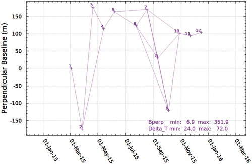
As shown in Figure 5, we constrained our SBAS network to interferometric pairs with perpendicular baselines varying between 6 and 352 m, which were smaller than the critical baseline of C-band. A coherence variation analysis was carried out to select interferometric pairs that have been less affected by temporal decorrelation. The results of this analysis showed that coherence can be maintained for a 72-day interval during the thawing season (July to October). However, coherence was only preserved for a 24-day interval in the early spring and freezing season.

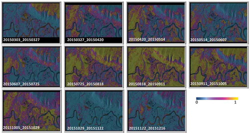
The outputs from InSAR processing were the coherence imagery and displacement map, which were used in Step 2 and Step 3, respectively. In particular, coherence images were produced in Step 1 and the high-coherence imagery, corresponding to July, August, September, and October were used as the input features for classification in the next step.

4.2. Object-based image analysis (step 2)

An Object-Based Image Analysis (OBIA) framework was developed for land cover classification. The object-based approach has advantages over the pixel-based approach since the former incorporates different input features (e.g., object size and shape), multiple sources of data with different spectral and spatial resolution, and the spatial and hierarchical relationship between neighbouring pixels rather than a single pixel (Mahdianpari et al. 2018). Thus, significant improvement in terms of extracted information for a given area is obtained using the OBIA technique. The first step in OBIA is multi-resolution segmentation (MRS). The multi-resolution segmentation available in eCognition Developer software package (V.9.0) (eCognition Developer, 2014) was used for this work. The multi-resolution segmentation was carried out using Sentinel-2 optical data rather than SAR imagery because the inherent speckle noise in SAR produces less well-defined objects and such data have relatively low ground-feature distinguishability (Mahdianpari et al. 2017c; Salehi, Daneshfar, and Davidson 2017). Multi-resolution segmentation is controlled by three user defined parameters, namely scale, shape, and compactness. Scale is the most crucial parameter affecting the size of objects or segments. While the eCognition default values were used for shape and compactness (0.1 and 0.5), a scale parameter of 300, which was obtained using a trial-and-error procedure, was found to be appropriate for this study according to the visual analysis of the segmentation results

The next step was feature extraction from Sentinel-2 and RADARSAT-2 data. Extracted features from the optical data were the Normalized Difference Vegetation Index (NDVI), Normalized Difference Water Index (NDWI), and 10 spectral bands of Sentinel-2. Although SAR imagery was not included in the multi-resolution segmentation step, the polygons resulted from the segmentation of the optical image were superimposed on SAR imagery and several SAR features were extracted for each polygon (segment). In particular, SAR features, including backscatter intensity and interferometric coherence images within the July to October timeframe, were extracted and used as input features for the classification scheme. The interferometric coherence maps were used as classification inputs to augment the information of SAR intensity (Mohammadimanesh et al. 2018a, 2018b). This is because SAR intensity depends on the electromagnetic structure of the targets while interferometric coherence represents the mechanical stability of the ground targets and is more sensitive to ground changes relative to SAR intensity. Thus, the synergistic use of two feature types enhances thematic land-cover information (Ramsey et al., 2006).

Random Forest (RF) is a non-parametric classifier independent of the input data distribution (Breiman 2001). Since our input data were from different sources (e.g., optical and SAR imagery) using a parametric classifier such as Maximum Likelihood classification, which assumes the normal distribution of data, is not effective (Salehi, Daneshfar, and Davidson 2017, Rezaee et al. 2018). The RF classifier is an ensemble of the Decision Tree (DT) classifier, each tree of which is trained on a randomly chosen subset of the input data, where the final classification is based on the majority vote of trees (Mahdianpari et al. 2018b). Also, RF is easily adjustable using two input variables, namely the number of trees (Ntree) and the number of variables (Mtry) (Mahdianpari et al. 2017c). In this study, a total number of 500 trees were selected for Ntree and the square root of the number of input variables (i.e., the default value) was selected for Mtry.

4.3. Permafrost analysis (step 3)

In Step 3, the relationships between the deformation map obtained from the SBAS InSAR analysis (Step 1), the land cover classification map (Step 2), and the geological features were examined. The two most relevant components of the surficial geology map, namely geomorphological processes and surface materials, were used to interpret the observed deformation. Generally, geomorphological processes are defined as the natural mechanisms of erosion, weathering, and deposition that modify surface material and landforms. Table 2 lists the geomorphological units and the percentage of the area that they cover in the study region (i.e., the percent coverage; Kennedy 2011).

Table 2. Geomorphological units and their percent coverage in the study area (Kennedy 2011).

Geomorphological unit	Description	Percent coverage
E	Channels formed by meltwater due to glaciers or ice sheets	2%
I	Irregular sinuous channels, which turn and bend without repetition of the same features	0%
B	A subclass of I where small channels may or may not be connected to the main channels	1.8% (Class Ib+ B)
L	Landslide processes; slow or rapid downslope movements such as sliding, falling, rolling, flowing, or creeping	0%
K	A subclass of L with tension cracks	0.2% (Class Lk)
X	Permafrost aggradation or degradation	23%
T	A subclass of X indicating thermokarst, which is subsidence due to thawing of ice-rich permafrost	32.5% (Xt)
Non	Unknown geomorphological processing unit	40.5%

The descriptions of I and L are included in this table; however, they are not discrete classes in the study area.

Surface materials in the study area consist of unconsolidated sediments produced by weathering, sediment deposition, human activity, and biological accumulation (Kennedy 2011). Table 3 lists the surface materials and their percent coverage in the region (Kennedy 2011). The surficial geology map for the study area covered only a portion of the SAR image; therefore, the interpretation of the results was limited to the portion of the InSAR displacement map covered by the surficial geology map (see Figure 1).

Table 3. Surface material units and their percent coverage in the study area (Kennedy 2011).

Surface material	Description	Percent coverage
Anthropogenic	Artificial or geological materials modified by human activities.	1%
Colluvium	Materials transported by direct, gravity-induced movement, including massive, moderately well-stratified, non-sorted to poorly sorted sediments of various particle sizes and types (i.e., from clay to boulders).	2%
Eolian	Materials transported or deposited by wind, including medium to fine sand and well-sorted coarse silts.	1.4%
Fluvial (active)	Materials transported by streams and rivers. These deposits consist of stratified beds of gravel, silt and/or organic materials.	1.9%
Fluvial (inactive)	Materials transported by streams and rivers. These deposits consist of stratified beds of gravel, silt and/or organic materials.	20%
Glaciofluvial	Materials deposited by glacial meltwater, ranging from non-sorted to non-bedded gravel with a wide range of particle sizes.	34.2%
Glaciolacustrine	Materials deposited in, or along, the margin of glacial lakes, including sediments released by the melting of the floating ice. They consist of stratified fine sand, silt, and clay.	14.9%
Moraine	Materials deposited directly by a glacier or ice sheet and characterized by poorly sorted, weakly compact materials lacking stratification that contain a heterogeneous mixture of particle sizes, including salt, silt, and clay.	20.1%
Organic	Materials found in low-lying areas where wet ground conditions facilitate a thick accumulation of vegetation.	4.5%

5. Results and discussion

Figure 6 shows the coherence images produced for the repeat-pass orbit, cycle to cycle image pairs of RADARSAT-2 from March to December 2015. Overall, these coherence maps demonstrate variability related to seasonal changes. The July to October image pairs illustrate better coherence preservation, while the April-May and November-December timeframes illustrate marginally lower coherence. This is likely due to snow melt (patchy wet snow) and vegetation growth in April and May (i.e., the melting season), as well as snow accumulation and high wind speed in November and December (i.e., the freezing season; Chu and Lindenschmidt 2017). Therefore, the most accurate and reliable deformation results were obtained using the July to October time interval. These observations are in general agreement with those reported in Short et al. (2011), who concluded that June to September datasets were most useful for InSAR processing of permafrost terrain on Herschel Island located off the northern Yukon coast. Other studies also reported the suitability of SAR observations during the thaw season for permafrost mapping using the InSAR technique (Wang and Li 1999; Rudy et al. 2018). This is because both accumulation and melt of snow during freezing (e.g., December) and melting (e.g., April) seasons result in surface changes and, accordingly, coherence loss. Snow moisture content is another factor affecting the coherence because it alters the dielectric constant of the ground targets. Accordingly, the upcoming RADARSAT Constellation Mission (RCM), with a temporal resolution of four days, will be significantly beneficial for monitoring phenomena with such high variability by reducing temporal decorrelation (Mahdianpari et al. 2017b).

Figure 6. Examples of interferometric coherence with the smallest temporal baseline from March to December 2015. Note that interferometric coherence ranges from 0 (no coherence) to 1 (perfect coherence).

Figure 7 shows the displacement map generated using the SBAS InSAR technique. The deformation results are relative to the InSAR reference point, which is assumed to be stable (i.e., the red star in Figure 7). A total of 66 interferograms were produced using 12 RADARSAT-2 SLC images. Among these, only 18 had a significant areal distribution of coherence for generating deformation results (i.e., above the threshold of 0.2). Overall, all land cover classes within the 18 selected interferograms, excluding the water class, had coherence greater than 0.2 across the entire study area.

Figure 7. Displacement map obtained from the SBAS InSAR technique (March 3 – 16 December 2015) overlying on the Sentinel-2 optical image (band 4) for the village area and Mayo Airport (Top) and the whole region (Bottom).

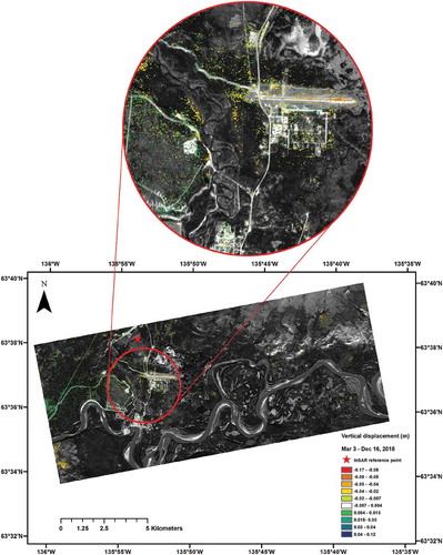
The displacement map shows subsidence beneath the airstrip with values predominantly ranging between −2 and −4 cm. Other areas affected by subsidence are found in the north-east and the south-west of the study area, outside of the red circle. However, there are some areas with uplift on the order of 0.4 to 3 cm in the western and southern parts of the upper panel image, mainly in paved areas (see also Figure 8(A). Thus, there is a possibility that these uplifts were related to anthropogenic surface modifications, such as road repairs and maintenance operations that occurred during satellite SAR acquisition. This is because repairs cause slight uplift of the ground surface by introducing gravel patches and asphalt layers.

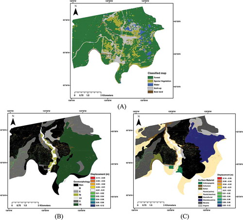
Figure 8. (A) Land cover classification map illustrating five major classes and (B) true color composite of Sentinel-2 optical image (bands 4, 3, and 2).

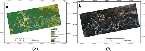
Figure 8(A) shows the land cover map generated by the object-based random forest classification using 21 input features (both optical and SAR features). A visual comparison between the classified map and the optical imagery shows that most land cover classes have been correctly classified (e.g., roads, building, and water). Table 4 shows the confusion matrix for this classified map.

Table 4. Confusion matrix for the classified map presentenced in Figure 8(A). An overall classification accuracy of 83.47% and Kappa coefficient of 0.76 were obtained.

		Classified data
		Forest	Sparse vegetation	Water	Built-up	Bare land	Tot.	Prod. Acc.
Reference data	Forest	68,497	8319	267	1649	3491	82,223	83.31
	Sparse vegetation	6532	31,107	105	1347	1479	40,570	76.67
	Water	66	131	28,258	459	221	29,135	96.99
	Built-up	1148	1016	305	8781	198	11,448	76.70
	Bare land	883	1284	219	366	12,309	15,061	81.73
	Tot.	77,126	41,857	29,154	12,602	17,698	178,437
	User. Acc.	88.81	74.32	96.93	69.68	69.55

The overall classification accuracy was 83.47%, with water correctly classified in 97% of cases, forest in 83%, bare land in 82%, and built-up and sparse vegetation in 77% of cases. The largest confusion was found for both sparse vegetation and built-up, which had the highest omission error. In particular, sparse vegetation was misclassified as forest and, to a lesser degree, the bare land class. This, too, occurred for the built-up class, which was erroneously classified as either forest or sparse vegetation (omission error). The largest commission error, however, was found for both built-up and bare land classes, wherein forest and sparse vegetation were misclassified as built-up and bare land. One possible reason for confusion between bare land and sparse vegetation was that these classes are mixed and lack clear-cut borders. These classes were also hardly distinguishable using satellite imagery during preparation of the reference polygons. The low accuracy of the built-up class could also be attributed to the low availability of training samples included for this class relative to other land cover types in this study (see Table 1).

Figure 9 shows the land cover classification map and two relevant components of a surficial geology map with an overlay of the SBAS InSAR deformation results.

Figure 9. (A) The land cover classification map, (B) the geomorphological process map with an overlay of the SBAS InSAR deformation results, and (C) the surface material map with an overlay of the SBAS InSAR results. Note that the dominant surface material component is used for the purpose of illustration.

The geomorphological process map includes seven classes presented and described in Table 2. As shown in Figure 9(B), the geomorphological processes in the eastern regions are permafrost or thermokarst. The InSAR results show a general trend of subsidence, which is in agreement with the expected movement for this geomorphological unit. For example, the unit corresponding to the eastern portion of the runway is thermokarst, a subclass of permafrost defined as a ground-surface depression caused by the thawing of ice-rich permafrost and associated soil subsidence (Kennedy 2011).

Figure 10 shows the area affected by movements for each geomorphological unit. Note that areas exhibiting a deformation range between −1 and 1 cm were considered stable and were not included in Figure 10(A) for better visualization. This was because most of the areas in all classes (i.e., greater than 95% per unit area) fall within this displacement range, as shown in Figure 10(B). It is also worth noting that different geomorphological units cover varying proportion of the study area. For example, the X and Xt classes cover a large portion of the study area (~55%), whereas some classes, such as E and B, cover a much smaller portion (less than 4%).

Figure 10. Histograms of displacement range vs. unit area for all geomorphological units. For example, [−14, −6] indicates displacement within the range of −6 to −14 cm. Negative and positive values represent subsidence and uplift, respectively. (A) All possible displacement ranges, excluding [−1, + 1] and (B) displacement within the [−1, + 1] range, representing stable areas. Note that a large portion (i.e., 95%) of different geomorphological units falls within the stable area. The two graphs (A and B) are complementary to each other.

In general, the InSAR displacement trends align well with the geomorphological map. Figure 10(A) shows that among all classes, X and E have the largest unit areas affected by displacement. These two classes correspond to permafrost and channels formed by meltwater from glaciers or ice sheets. However, subsidence greater than −4 cm predominantly occurred in permafrost regions (class X; see Figure 10(A)). Although class E demonstrated relatively high deformation, it only covers a small portion (2%) of the study region relative to class X (23%).

Unfortunately, the geomorphological unit for a large portion of the study area is unknown according to the geomorphological map (Non-class; see Figure 9(B)). However, our InSAR results indicate surface deformation in these areas, which may or may not be related to permafrost activity. Thus, a surface material map was also used for further investigation. Figure 9(C) shows the surface material map overlaying by the SBAS InSAR results.

Fluvial, glaciofluvial, moraine, and glaciolacustrine sediments are the dominant surface materials in the study area (see Figure 9(C) and Table 3). Figure 11(A) shows the unit area affected by the movement of these materials in the study area. Note that the areas exhibiting a deformation range between −1 and 1 cm were considered stable and, accordingly, were not included in Figure 11(A) for visualization purpose.

Figure 11. Histograms of displacement range vs. unit area for the dominant surface material unit. Negative and positive values represent subsidence and uplift, respectively. (A) All possible displacement ranges, excluding [−1, + 1] and (B) displacement within the [−1, + 1] range, representing stable areas.

As shown in Figure 11, displacement mainly occurred within glaciofluvial and moraine sediments. According to the Northern Climate Exchange (2011), glaciolacustrine materials, moraine deposits, and areas along the Stewart River are the least stable landforms in the Village of Mayo. The low stability along the Stewart River is due to erosion along the river bank. Moraine deposits are generally found to be stable; however, buried glacial ice or permafrost is potentially present in moraine deposits due to their poor drainage capabilities. Moraines are generally characterized by poorly sorted, less compact materials that are usually fine-grained and very susceptible to water retention and, as such, are thaw sensitive.

The InSAR results identified glaciofluvial materials as unstable sediments. This class approximately corresponds to the non-class in the geomorphological map (see Figure 9(B–C)). These materials were deposited by glacial meltwater through direct or indirect contact with glacier ice. Short et al. (2014) also reported the existence of ice wedges and massive ice bodies in glaciofluvial sediments, which caused localised instability in the permafrost region in Iqaluit, Baffin Island, Canada. Therefore, glaciofluvial materials may be attributed to past glacial activity and, as such, there is a potential for permafrost in these sediments.

Importantly, our InSAR results show instability at the eastern end of the Mayo Airport. This area consists of glaciolacustrine silt and clay, and although these materials are not exposed on the surface, their presence is indicated by several hollows (depressions and thermokarst landforms; Northern Climate Exchange 2011). This conclusion is in agreement with Kennedy, Lipovsky, and Benkert (2014), who pointed out that much of the main infrastructure in the Village of Mayo (e.g., the airport and school) is underlain by interbedded glaciolacustrine and glaciofluvial sediments. The Northern Climate Exchange (2011) and Kennedy, Lipovsky, and Benkert (2014) also reported that submission of glaciolacustrine sediments caused the most damage to human-made structures in the Village of Mayo. The existence of glaciolacustrine sediments as the second dominant component beneath the airstrip according to the surficial geology map also supports their presence at the Mayo Airport site (Kennedy 2011). Importantly, glaciolacustrine sediments are deeply deposited and are not exposed on the ground surface. This indicates the necessity of sub-surface investigation to accurately identify their spatial distribution (Northern Climate Exchange 2011), as it may be underestimated in the surficial geology map. Similar results were also reported in Yellowknife, Northwest Territories, which is located within the extensive discontinuous permafrost zone. In particular, Wolfe et al. (2014) found instability within glaciofluvial sediments and reported the possibility that glaciolacustrine deposits underlie unstable regions of glaciofluvial sediments identified in their InSAR displacement map.

Figure 12 shows the unit area affected by varying degrees of displacement for each land-cover type. Forest, sparse vegetation, built-up, water, and bare land cover an approximate area of 69%, 15.5%, 10.5%, 3.5%, and 1.5% of the study area shown in Figure 9(A), respectively. Note that the aforementioned values are the percentage of areas covered by each land-cover type in the study region. This is different from the unit areas indicated in Figure 12 because the sum of all unit areas for each individual class in this figure is 100%. For example, approximately 95% of bare land is within stable zone of the [−1, + 1] (Figure 12(B)) which covers approximately 1.4% (i.e., 95% x 1.5%) of the entire study area.

Figure 12. Histograms of displacement range vs. unit area for different land-cover classes of (A) all possible displacement ranges, excluding [−1, + 1], and (B) displacement within the [−1, + 1] range, representing stable areas.

There are several interesting observations from the histograms in Figure 12. First, Figure 12 (B) shows that the majority of each land cover class is within the stable zone ([−1, + 1] cm). Among the four classes, bare land and built-up have the smallest unit areas within the stable zone (less than 94% and 95% for built-up and bare land, respectively). Figure 12(A) also reveals that, of the approximate 5% unit area of bare land located outside the stable zone, about 2.6% includes uplift that ranges between 1 and 4 cm and about 1.5% is within the −1 to −4 cm displacement (subsidence) range. For the built-up class, about 6% of the unit area is within the unstable zone, with 2.8% in the 1 to 4 cm uplift range and 2.7% in the −1 to −4 cm subsidence range. Although these two classes cover a small part of the study area (i.e., 10.5% built-up and 1.5% bare land), they are the most affected by displacement. This can be explained by the fact that bare land is more exposed to the weather and temperature changes and, consequently, the seasonal freezing and thawing of the active layer overlaying the permafrost. In addition, the instability of built-up areas (e.g., forest clear cuts, roads, villages, and airports) is likely due to the reduction of vegetation and other anthropogenic interferences (e.g., building construction). This is confirmed, visually, in Figure 7 (Top panel), where an uplift displacement pattern is seen on the gravel road in the left of the image. Figure 12(B) shows that about 3% of forest and 2.5% of sparse vegetation are within displacement zones beyond $\pm$1 cm (i.e., unstable area). These two classes cover approximately 84.5% of the study area (Figure 9(A)). Notably, the total area of the study shown in Figure 9(A) is about 58 km², of which 49 km² is covered by the forest and sparse vegetation classes. Thus, the total areas of these two classes with displacement larger than $\pm$1 cm are 1.2 and 0.22 km² for forest and sparse vegetation, respectively.

6. Evaluation of the SBAS InSAR results

Unfortunately, a field survey was not conducted as part of this research to quantitatively validate the InSAR results. This is attributable to the remoteness, vastness, and harsh environmental conditions of permafrost areas (Short et al. 2011; Wang et al. 2017). However, a recent study, carried out by the Northern Climate Exchange (2011) in the summer of 2010, allows some evaluation of the InSAR results. The objective of the Northern Climate Exchange (2011) study was to create a hazard map of the community of Mayo to determine threats due to changes in the landscape and underlying sediment. The Northern Climate Exchange (2011) surveyed several locations in the area to examine permafrost conditions. Electrical resistivity profiles were also collected from several sites because permafrost has a distinct electrical signature, wherein the freezing of water decreases the availability of pore fluid for electrical conduction (Short et al. 2014). As such, frozen regions have a high resistivity, whereas unfrozen ground within the permafrost regions has relatively low resistivity. Resistivity profiling can, therefore, be used to characterize the relationship between the InSAR results and the frozen or unfrozen status of the ground.

The first location, J.V. Clark School, lies on a site that has experienced several decades of permafrost disturbance (Northern Climate Exchange 2011). The location of the school is marked as point 1 in Figure 1. Field investigations confirmed the existence of permafrost with a relatively thin active layer in the forested areas adjacent to the school. Resistivity surveys were conducted at two locations: the extreme north and the north-eastern sections of the school. The northern survey confirmed the presence of permafrost with a thickness between 5 and 7 m. The permafrost in this area is possibly warm and, as such, susceptible to thaw given its thickness. The survey of the north-eastern part of the school extended from a disturbed forested region into a less disturbed area and indicated the presence of permafrost with a depth greater than 25 m in the latter area. This could be attributed to the undisturbed vegetation and forest effectively insulating the permafrost, resulting in its preservation. Additionally, a talik (i.e., a perennially thawed zone) located within the disturbed area appeared to be the result of vegetation disturbance. Figure 13 (Top panel) shows the time series of vertical displacement for the two points marked in Figure 1.

Figure 13. (Top panel) The SBAS InSAR time series of vertical displacement for the time interval between March to December 2015 for site 1 located at the north-east of J.V. Clark School and site 2 located at the east of the Mayo Airport. (Bottom panel) (A) and (B) are Google Earth images showing the location of sites 1 and 2, and (C) is a photograph illustrating a frost crack at the Mayo Airport (Northern Climate Exchange 2011).

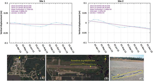
RADARSAT-2 results from the summer of 2015 indicate movements of −1 to −1.5 cm to the north-east of the school (site 1). These values demonstrate a small degree of subsidence due to seasonal settlement of the active layer. The range of variation for this site over the summer seems realistic given the permafrost thickness in this region and the short time interval.

The second field investigation took place at the eastern end of the Mayo airstrip. This site is marked as point 2 in Figure 1. Ground settlement was reported in the areas surrounding the Mayo Airport (Northern Climate Exchange 2011; see also Figure 13(C)). The main factors contributing to the degradation of permafrost under the runway are the reduction of vegetation and organic material during airport construction and the flowing of ground water beneath the runway (Northern Climate Exchange 2011). A long resistivity survey (320 m) was carried out from the thermokarst area to the east and up a low ridge to the southern portion of the Mayo airstrip. The results indicated that permafrost extends 25 m beneath the ridge and contains ice-rich sediments at depths of 10 to 15 m. Permafrost adjacent to the airstrip had also degraded near the surface, creating a talik (Northern Climate Exchange 2011). Figure 13 (top panel-site 2) shows the time series of movements for the east end of the Mayo airstrip.

Although there is a time gap between our InSAR observations (2015) and the resistivity profiling (2010), there is consistency between the two studies. For example, the 2015 InSAR results show a general trend of subsidence at the eastern portion of the Mayo airstrip, likely indicating degradation of the underlying permafrost. This was corroborated by resistivity profiling illustrating that much of the ground beneath the Mayo airstrip, especially the eastern section, had low resistivity (i.e., unfrozen) at the time of field observation (Northern Climate Exchange 2011). Also, the time series of deformation for site 1 (school) reveals only seasonal variation in the active layer with negligible movement during a one-year interval. Resistivity profiling also demonstrated that a large portion of ground in the northeast of the school had high resistivity (i.e., frozen condition) at the time of field observation (i.e., summer 2010; Northern Climate Exchange 2011).

Overall, the time series of vertical displacement at both sites in Mayo shows seasonal variation, which is primarily due to the settlement and heave of ground ice in the active layer during the thaw and freezing seasons, respectively. During the thaw season, the surface subsides because ground ice within the active layer melts, causing a volume decrease and soil consolidation. In contrast, during the freezing season, the surface uplifts due to the transformation of water to ice, resulting in frost heave (Rudy et al. 2018). The Northern Climate Exchange (2011) reported that ground ice contents of permafrost ranged from low to moderate at most of the Mayo visited-sites. However, ice-rich sediments are also found in the Mayo area. This potentially occurs within glaciolacustrine sediments, since they are characterized by fine sediments with high ice contents and massive ice lenses in the Mayo region (Burn, Michel, and Smith 1986). Importantly, the eastern end of the Mayo airstrip is interbedded with glaciolacustrine and glaciofluvial sediments (Kennedy, Lipovsky, and Benkert 2014). Accordingly, the degradation of permafrost in this location (site 2) could be attributed to the high ice contents (moisture) within glaciolacustrine sediments.

Notably, the time series of displacement for both sites primarily shows negative values during the summer (June-August), representing downward movement related to thaw resulting from an increase in air temperature (see Figure 2). Specifically, these observations suggest that thaw begins as early as May, indicating a correlation with the increase in air temperature during that time. As temperatures decrease, by early autumn (September) the ground begins to refreeze, causing surface uplift.

Similar to Li et al. (2003) and Short et al. (2011), the results of this research illustrate that the spatial pattern of permafrost variations can be identified using InSAR. The evaluation of the InSAR measurements demonstrates that the results are qualitatively correct and realistic for a one-year time interval; however, simultaneous and detailed fieldwork is necessary to quantitatively validate the deformations identified using InSAR in this area.

7. Conclusion

The impact of climate change on permafrost poses significant challenges for northern communities. Climate-related degradation of the permafrost layer often results in the subsidence of overlying material, which potentially causes damage to infrastructure founded in these regions. This indicates the importance of adapting to climate change in northern regions by identifying vulnerable areas so that mitigation plans can be put into place to limit damages to infrastructure and to direct maintenance activities.

In this study, the SBAS InSAR technique was integrated with an object-based image analysis to identify ground instability due to permafrost activity in the center of the Yukon Territory, Canada. The classification results showed that deformation occurred in almost all classes, excluding the water class. It also illustrated that subsidence was the dominant movement for the built-up class. Two relevant components of the surficial geology map, namely geomorphological processes and surface materials, were used to interpret and qualitatively evaluate the InSAR results. The results of this analysis revealed that the spatial extent of the displacement map obtained from the SBAS InSAR technique to be correlated with the surficial geology map. Specifically, unstable regions identified by InSAR were associated with moraine, glaciofluvial, and glaciolacustrine sediments, the latter of which is not exposed on the ground surface.

The results of this research advance an operational monitoring of permafrost and offer valuable information for those landscapes affected by permafrost. It also serves as a baseline guide for establishing adaptation and mitigation plans and may be used for further scientific research in this and other cold regions with similar climatic characteristics.

Acknowledgements

This work was part of a larger project funded by Defence Research and Development Canada (DRDC) through the Defence Innovation Research Program (DIRP). The authors greatly appreciated comments and suggestions from DRDC Ottawa scientist, including Dr. Karim Mattar and Dr. Paris Vachon. Also, the authors would like to thank five anonymous reviewers for their helpful comments and suggestions.

Disclosure statement

No potential conflict of interest was reported by the authors.

Notes

1. Canadian Census 2016: http://www12.statcan.gc.ca/.

References

- Antonova, S., A. Kääb, B. Heim, M. Langer, and J. Boike. 2016. “Spatio-Temporal Variability of X-Band Radar Backscatter and Coherence over the Lena River Delta, Siberia.” Remote Sensing of Environment 182: 169–191. doi:10.1016/j.rse.2016.05.003.
- Berardino, P., G. Fornaro, R. Lanari, and E. Sansosti. 2002. “A New Algorithm for Surface Deformation Monitoring Based on Small Baseline Differential SAR Interferograms.” IEEE Transactions on Geoscience and Remote Sensing 40 (11): 2375–2383. doi:10.1109/TGRS.2002.803792.
- Bleiler, L., C. Burn, and M. O’Donoghue, eds. 2006. Heart of the Yukon: A Natural and Cultural History of the Mayo Area, 138. Mayo, YT: Village of Mayo.
- Breiman, L. 2001. “Random Forests.” Machine Learning 45 (1): 5–32. doi:10.1023/A:1010933404324.
- Burn, C. R. 2000. “The Thermal Regime of a Retrogressive Thaw Slump near Mayo, Yukon Territory.” Canadian Journal of Earth Sciences 37 (7): 967–981. doi:10.1139/e00-017.
- Burn, C. R., F. A. Michel, and M. W. Smith. 1986. “Stratigraphic, Isotopic, and Mineralogical Evidence for an Early Holocene Thaw Unconformity at Mayo, Yukon Territory.” Canadian Journal of Earth Sciences 23 (6): 794–803. doi:10.1139/e86-081.
- Burn, C. R., and P. A. Friele. 1989. “Geomorphology, Vegetation Succession, Soil Characteristics and Permafrost in Retrogressive Thaw Slumps near Mayo, Yukon Territory.” Arctic Vol. 42, No. 1 (Mar., 1989), pp.31–40.
- Chen, F., H. Lin, W. Zhou, T. Hong, and G. Wang. 2013. “Surface Deformation Detected by ALOS PALSAR Small Baseline SAR Interferometry over Permafrost Environment of Beiluhe Section, Tibet Plateau, China.” Remote Sensing of Environment 138: 10–18. doi:10.1016/j.rse.2013.07.006.
- Chen, F., H. Lin, Z. Li, Q. Chen, and J. Zhou. 2012. “Interaction between Permafrost and Infrastructure along the Qinghai–Tibet Railway Detected via Jointly Analysis of C-And L-Band Small Baseline SAR Interferometry.” Remote Sensing of Environment 123: 532–540. doi:10.1016/j.rse.2012.04.020.
- Chen, W. F., H. L. Gong, B. B. Chen, K. S. Liu, M. Gao, and C. F. Zhou. 2017. “Spatiotemporal Evolution of Land Subsidence around a Subway Using InSAR Time-Series and the Entropy Method.” GIScience & Remote Sensing 54 (1): 78–94. doi:10.1080/15481603.2016.1257297.
- Chu, T., and K. E. Lindenschmidt. 2017. “Comparison and Validation of Digital Elevation Models Derived from InSAR for a Flat Inland Delta in the High Latitudes of Northern Canada.” Canadian Journal of Remote Sensing 43 (2): 109–123. doi:10.1080/07038992.2017.1286936.
- Dehghan-Soraki, Y., M. Sharifikia, and M. R. Sahebi. 2015. “A Comprehensive Interferometric Process for Monitoring Land Deformation Using ASAR and PALSAR Satellite Interferometric Data.” GIScience & Remote Sensing 52 (1): 58–77. doi:10.1080/15481603.2014.989774.
- Deng, Z., Y. Ke, H. Gong, X. Li, and Z. Li. 2017. “Land Subsidence Prediction in Beijing Based on PS-InSAR Technique and Improved Grey-Markov Model.” GIScience & Remote Sensing 54 (6): 797–818. doi:10.1080/15481603.2017.1331511.
- eCognition Developer, T. 2014. 9.0 User Guide. Munich, Germany: Trimble Germany GmbH.
- Fariba Mohammadimanesh, Bahram Salehi, Masoud Mahdianpari , Brian Brisco & Mahdi Motagh., (2018c), Wetland Water Level Monitoring Using Interferometric Synthetic Aperture Radar (InSAR): A Review, Canadian Journal of Remote Sensing, in press. DOI:10.1080/07038992.2018.1477680
- Ferretti, A., A. Monti-Guarnieri, C. Prati, F. Rocca, and D. Massonet. 2007. InSAR Principles-Guidelines for SAR Interferometry Processing and Interpretation. Vol. 19. The Netherlands: ESA Publications.
- Ferretti, A., C. Prati, and F. Rocca. 2000. “Nonlinear Subsidence Rate Estimation Using Permanent Scatterers in Differential SAR Interferometry.” IEEE Transactions on Geoscience and Remote Sensing 38 (5): 2202–2212. doi:10.1109/36.868878.
- Fiaschi, S., S. Tessitore, R. Bonì, D. Di Martire, V. Achilli, S. Borgstrom, A. Ibrahim, et al. 2017. “From ERS-1/2 to Sentinel-1: Two Decades of Subsidence Monitored through A-DInSAR Techniques in the Ravenna Area (Italy).” GIScience & Remote Sensing 54 (3): 305–328. doi:10.1080/15481603.2016.1269404.
- Hall-Atkinson, C., and L. C. Smith. 2001. “Delineation of Delta Ecozones Using Interferometric SAR Phase Coherence: Mackenzie River Delta, NWT, Canada.” Remote Sensing of Environment 78 (3): 229–238. doi:10.1016/S0034-4257(01)00221-8.
- Heginbottom, J. A., M. A. Dubreuil, and P. T. Harker. 1995. “Permafrost Map of Canada.” The National Atlas of Canada, 5th Edition,(1978-1995), Published by Natural Resources Canada, Sheet MCR 4177 (1): 7.
- Hennessey, R., S. Stuart, and F. Duerden. 2012. Mayo Region Climate Change Adaptation Plan.Northern Climate ExChange, 103. Whitehorse, YT: Yukon Research Centre, Yukon College.
- Karunaratne, K. C., and C. R. Burn. 2004. “Relations between Air and Surface Temperature in Discontinuous Permafrost Terrain near Mayo, Yukon Territory.” Canadian Journal of Earth Sciences 41 (12): 1437–1451. doi:10.1139/e04-082.
- Kennedy, K., P. Lipovsky, and B. Benkert. 2014. “Geoscience Mapping for Climate Change Adaptation Planning: Landscape Hazard Maps as a Tool for Communities in Yukon, Canada.” 2014 GSA Annual Meeting in Vancouver, October, British Columbia.
- Kennedy, K. E., 2011. “Surficial Geology of the Village of Mayo (Part of NTS 105M/12) Yukon.” Yukon Geological Survey Open File 2011-3, 1:20 000 scale.
- Li, S. S., V. Romanovsky, J. Lovick, Z. Wang, and R. Peterson, 2003. Application of satellite SAR imagery in mapping the active layer of Arctic permafrost. Final Report NAG5- 8614 : NASA Centre for Aerospace Information, United States.
- Mahdianpari, M., B. Salehi, and F. Mohammadimanesh. 2017a. “The Effect of PolSAR Image De-Speckling on Wetland Classification: Introducing a New Adaptive Method.” Canadian Journal of Remote Sensing 43 (5): 485–503. doi:10.1080/07038992.2017.1381549.
- Mahdianpari, M., B. Salehi, F. Mohammadimanesh, and B. Brisco. 2017b. “An Assessment of Simulated Compact Polarimetric SAR Data for Wetland Classification Using Random Forest Algorithm.” Canadian Journal of Remote Sensing 43 (5): 468–484. doi:10.1080/07038992.2017.1381550.
- Mahdianpari, M., B. Salehi, F. Mohammadimanesh, B. Brisco, S. Mahdavi, M. Amani, and J. E. Granger. 2018. “Fisher Linear Discriminant Analysis of Coherency Matrix for Wetland Classification Using PolSAR Imagery.” Remote Sensing of Environment 206: 300–317. doi:10.1016/j.rse.2017.11.005.
- Mahdianpari, M., B. Salehi, F. Mohammadimanesh, and M. Motagh. 2017c. “Random Forest Wetland Classification Using ALOS-2 L-Band, RADARSAT-2 C-Band, and TerraSAR-X Imagery.” ISPRS Journal of Photogrammetry and Remote Sensing 130: 13–31. doi:10.1016/j.isprsjprs.2017.05.010.
- Mahdianpari, M., Salehi, B., Rezaee, M., Mohammadimanesh, F. and Zhang, Y., (2018). Very Deep Convolutional Neural Networks for Complex Land Cover Mapping Using Multispectral Remote Sensing Imagery. Remote Sensing, 10, p.1119.
- Mohammadimanesh, F., B. Salehi, M. Mahdianpari, B. Brisco, and M. Motagh. 2018a. “Multi-Temporal, Multi-Frequency, and Multi-Polarization Coherence and SAR Backscatter Analysis of Wetlands.” ISPRS Journal of Photogrammetry and Remote Sensing 142: 78–93. doi:10.1016/j.isprsjprs.2018.05.009.
- Mohammadimanesh, F., Salehi, B., Mahdianpari, M., Motagh, M. and Brisco, B.., 2018b. An efficient feature optimization for wetland mapping by synergistic use of SAR intensity, interferometry, and polarimetry data. International Journal of Applied Earth Observation and Geoinformation, 73, pp.450–462.
- Muller, S. W. 1947. Permafrost or Permanently Frozen Ground and Related Engineering Problems. Ann Arbor, MI: J.W. Edwards Inc.
- Northern Climate Exchange, 2011. Mayo Landscape Hazards: Geological Mapping for Climate Change Adaptation Planning. Yukon Research Centre, Yukon College, 64 and 2 maps. Whitehorse, Yukon: Yukon Research Centre, Yukon College.
- Ramsey III, E., Z. Lu, A. Rangoonwala, and R. Rykhus. 2006. “Multiple Baseline Radar Interferometry Applied to Coastal Land Cover Classification and Change Analyses.” GIScience & Remote Sensing 43 (4): 283–309. doi:10.2747/1548-1603.43.4.283.
- Rezaee, M., Mahdianpari, M., Zhang, Y. and Salehi, B., (2018), Deep Convolutional Neural Network for Complex Wetland Classification Using Optical Remote Sensing Imagery. IEEE Journal of Selected Topics in Applied Earth Observations and Remote Sensing, (99).
- Rignot, E., and J. B. Way. 1994. “Monitoring Freeze—Thaw Cycles along North—South Alaskan Transects Using ERS-1 SAR.” Remote Sensing of Environment 49 (2): 131–137. doi:10.1016/0034-4257(94)90049-3.
- Rudy, A. C. A., S. F. Lamoureux, P. Treitz, N. Short, and B. Brisco. 2018. “Seasonal and Multi-Year Surface Displacements Measured by DInSAR in a High Arctic Permafrost Environment.” International Journal of Applied Earth Observation and Geoinformation 64: 51–61. doi:10.1016/j.jag.2017.09.002.
- Salehi, B., B. Daneshfar, and A. M. Davidson. 2017. “Accurate Crop-Type Classification Using Multi-Temporal Optical and Multi-Polarization SAR Data in an Object-Based Image Analysis Framework.” International Journal of Remote Sensing 38 (14): 4130–4155. doi:10.1080/01431161.2017.1317933.
- Short, N., A. M. LeBlanc, W. Sladen, G. Oldenborger, V. Mathon-Dufour, and B. Brisco. 2014. “RADARSAT-2 D-InSAR for Ground Displacement in Permafrost Terrain, Validation from Iqaluit Airport, Baffin Island, Canada.” Remote Sensing of Environment 141: 40–51. doi:10.1016/j.rse.2013.10.016.
- Short, N., B. Brisco, N. Couture, W. Pollard, K. Murnaghan, and P. Budkewitsch. 2011. “A Comparison of TerraSAR-X, RADARSAT-2 and ALOS-PALSAR Interferometry for Monitoring Permafrost Environments, Case Study from Herschel Island, Canada.” Remote Sensing of Environment 115 (12): 3491–3506. doi:10.1016/j.rse.2011.08.012.
- Smith, C. A. S., J. C. Miekle, and C. F. Roots, eds. 2004. Ecoregions of the Yukon Territory – Biophysical Properties of Yukon Landscapes. Agriculture and Agri-Food Canada, 313. Summerland, BC: PARC Technical Bulletin 04-01.
- Strozzi, T., U. Wegmuller, and C. Matzler. 1999. “Mapping Wet Snowcovers with SAR Interferometry.” International Journal of Remote Sensing 20 (12): 2395–2403. doi:10.1080/014311699212083.
- Suresh Krishnan, P. V., Duk-jin Kim, and Jungkyo Jung. 2018. “Subsidence in the Kathmandu Basin, before and after the 2015 Mw 7.8 Gorkha Earthquake, Nepal Revealed from Small Baseline Subset-DInSAR Analysis.” GIScience & Remote Sensing 55 (4): 604–621. doi:10.1080/15481603.2017.1422312.
- Throop, J., A. G. Lewkowicz, and S. L. Smith. 2012. “Climate and Ground Temperature Relations at Sites across the Continuous and Discontinuous Permafrost Zones, Northern Canada.” Canadian Journal of Earth Sciences 49 (8): 865–876. doi:10.1139/e11-075.
- Van Everdingen, R. O., ed. 1998. Multi-Language Glossary of Permafrost and Related Ground-Ice Terms in Chinese, English, French, German, Icelandic, Italian, Norwegian, Polish, Romanian, Russian, Spanish, and Swedish. Calgary: International Permafrost Association, Terminology Working Group.
- Wang, L., P. Marzahn, M. Bernier, A. Jacome, J. Poulin, and R. Ludwig. 2017. “Comparison of TerraSAR-X and ALOS PALSAR differential interferometry with multisource DEMs for monitoring ground displacement in a discontinuous permafrost region.” Ieee Journal of Selected Topics in Applied Earth Observations and Remote Sensing 10 (9): 4074-4093.
- Wang, Z., and S. Li, 1999. “Detection of Winter Frost Heaving of the Active Layer of Arctic Permafrost Using SAR Differential Interferograms.” In Geoscience and Remote Sensing Symposium, 1999. IGARSS’99 Proceedings. IEEE 1999 International, Vol. 4, 1946–1948. IEEE. Hamburg, Germany; 28 June-2 July 1999
- Wegmüller, U. 1990. “The Effect of Freezing and Thawing on the Microwave Signatures of Bare Soil.” Remote Sensing of Environment 33 (2): 123–135. doi:10.1016/0034-4257(90)90038-N.
- Weydahl, D. J. 2001. “Analysis of ERS Tandem SAR Coherence from Glaciers, Valleys, and Fjord Ice on Svalbard.” IEEE Transactions on Geoscience and Remote Sensing 39 (9): 2029–2039. doi:10.1109/36.951093.
- Wolfe, S. A., N. H. Short, P. D. Morse, S. H. Schwarz, and C. W. Stevens. 2014. “Evaluation of RADARSAT-2 DInSAR Seasonal Surface Displacement in Discontinuous Permafrost Terrain, Yellowknife, Northwest Territories, Canada.” Canadian Journal of Remote Sensing 40 (6): 406–422. doi:10.1080/07038992.2014.1012836.
- “Yukon Energy Mines and Resources.” “http://www.emr.gov.yk.ca/”.
- Zhao, R., Z. W. Li, G. C. Feng, Q. J. Wang, and J. Hu. 2016. “Monitoring Surface Deformation over Permafrost with an Improved SBAS-InSAR Algorithm: With Emphasis on Climatic Factors Modeling.” Remote Sensing of Environment 184: 276–287. doi:10.1016/j.rse.2016.07.019.
- Zhou, C., H. Gong, B. Chen, F. Zhu, G. Duan, M. Gao, and W. Lu. 2016. “Land Subsidence under Different Land Use in the Eastern Beijing Plain, China 2005-2013 Revealed by InSAR Timeseries Analysis.” GIScience & Remote Sensing 53 (6): 671–688. doi:10.1080/15481603.2016.1227297.