Reducing the effects of vegetation phenology on change detection in tropical seasonal biomes

Abstract

Tropical seasonal biomes (TSBs), such as the savannas (Cerrado) and semi-arid woodlands (Caatinga) of Brazil, are vulnerable ecosystems to human-induced disturbances. Remote sensing can detect disturbances such as deforestation and fires, but the analysis of change detection in TSBs is affected by seasonal modifications in vegetation indices due to phenology. To reduce the effects of vegetation phenology on changes caused by deforestation and fires, we developed a novel object-based change detection method. The approach combines both the spatial and spectral domains of the normalized difference vegetation index (NDVI), using a pair of Operational Land Imager (OLI)/Landsat-8 images acquired in 2015 and 2016. We used semivariogram indices (SIs) as spatial features and descriptive statistics as spectral features (SFs). We tested the performance of the method using three machine-learning algorithms: support vector machine (SVM), artificial neural network (ANN) and random forest (RF). The results showed that the combination of spatial and spectral information improved change detection by correctly classifying areas with seasonal changes in NDVI caused by vegetation phenology and areas with NDVI changes caused by human-induced disturbances. The use of semivariogram indices reduced the effects of vegetation phenology on change detection. The performance of the classifiers was generally comparable, but the SVM presented the highest overall classification accuracy (92.27%) when using the hybrid set of NDVI-derived spectral-spatial features. From the vegetated areas, 18.71% of changes were caused by human-induced disturbances between 2015 and 2016. The method is particularly useful for TSBs where vegetation exhibits strong seasonality and regularly spaced time series of satellite images are difficult to obtain due to persistent cloud cover.

Keywords:

• remote sensing
• geostatistics
• seasonality
• LULCC

1. Introduction

Tropical seasonal biomes (TSBs), such as savannas (also known as Cerrado) and semi-arid woodlands (also known as Caatinga), cover 35% of Brazil and consist of several vegetation types ranging from grasslands to forests (Silveira et al. 2018a). However, human-induced disturbances, such as deforestation and fires, are threatening these ecosystems (Silva et al. 2006; Hansen et al. 2013). In addition, because most of the conservation plans focus on moist evergreen tropical forests (Hoekstra et al. 2005), less attention has been dedicated to TSB areas (Beuchle et al. 2015).

TSBs experience seasonal changes in hydrological and nutrient conditions that affect the spectral signature of vegetation measured by satellites (Zhang, Ross, and Gann 2016). For instance, leaf area index (LAI) varies seasonally, having a maximum value during the rainy season and a minimum value during the dry season. Therefore, a seasonal fluctuation in the Normalized Difference Vegetation Index (NDVI) is generally observed over TSBs due to leaf shedding and increasing amounts of nonphotosynthetic vegetation during the dry season (Lagomasino et al. 2014). This NDVI behavior represents a challenge for land use and land cover change (LULCC) detection when multi-temporal images are used in the analysis.

Bi-temporal remote sensing images can be used to monitor vegetation and to detect changes caused by human and natural processes (Verbesselt et al. 2010; Zhu, Woodcock, and Olofsson 2012). However, in TSBs, phenology produces significant changes in vegetation conditions affecting the spectral response of vegetation (Wright and Van Schaik 1994). Even fixing a single period for image acquisition (rainy or dry season), the effects of vegetation phenology on LULCC detection are still significant due to the large seasonal and interannual variability in precipitation observed in TSBs.

Several methods have been proposed to reduce the effects of vegetation phenology on LULCC detection using time series of satellite images. Examples are the Breaks For Additive Seasonal and Trend algorithm (BFAST) (Verbesselt et al. 2010); Continuous Change Detection and Classification (CCDC) (Zhu and Woodcock 2014); Vegetation Change Tracker (VCT) (Huang et al. 2010); LandTrend (Kennedy, Yang, and Cohen 2010); Vegetation Regeneration and Disturbance Estimates through Time (VerDET) (Hughes, Kaylor, and Hayes 2017); and the Residual Trend Analysis (RESTREND) (Evans and Geerken 2004; Ibrahim et al. 2015). These methods usually require high-quality time series, which are not generally available over TSBs due to persistent cloud cover. Therefore, LULCC detection in complex landscapes, like those found in TSBs, still present a significant challenge (Healey et al. 2018).

Previous studies have shown that pixel-based change detection approaches can benefit from including information on spatial context (Chen et al. 2012; Hamunyela, Verbesselt, and Herold 2016). The neighborhood used to extract the spatial information is often defined by a square window that is easy to implement, however, they are computationally demanding (Zhu 2017), biased along their diagonals, and can straddle the boundary between two landscape features, especially when a large window size is used (Laliberte and Rango 2009). Using OBIA these problems are eliminated, allowing the inclusion of additional spatial information to improve remote sensing applications (Chen et al. 2018). For example, semivariograms of geostatistics have been widely used in image classification analyses (Balaguer et al. 2010; Silveira et al. 2017; Wu et al. 2015) and change detection studies (Gil-Yepes et al. 2016; Hamunyela et al. 2017; Silveira et al. 2018b). Thus, object-based methods that require only a few satellite images to reduce the effects of vegetation phenology on LULCC detection are needed to monitor TSB areas with persistent cloud cover and strong seasonality.

Here, to evaluate whether we can differentiate seasonal variations in NDVI values due to vegetation phenology from spectral variations associated with human-induced disturbances, we developed a novel object-based change detection (OBCD) approach. The objective was to reduce the effects of vegetation phenology on LULCC detection by combining spatial (i.e. semivariogram indices – SIs) and spectral information (i.e. spectral features – SFs). Our method does not require time series of satellite images because it exploits the spatial and spectral domains of NDVI, calculated from a pair of Operational Land Imager (OLI)/Landsat-8 images. Specifically, we tested the approach with three machine learning algorithms (MLAs), including support vector machine (SVM), artificial neural network (ANN) and random forest (RF) algorithms, to classify areas that experienced changes caused by vegetation phenology and human-induced disturbances

2. Study area

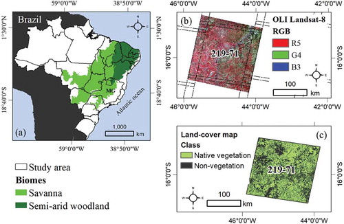
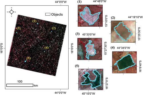
The study area is located in the north of Minas Gerais (MG) state, Brazil (Figure 1). In this area, the TSBs include Brazilian savannas (Cerrado) and semi-arid woodlands (Caatinga) (Figure 1a) (Scolforo et al. 2015). The study area is covered by the path 219 and row 71 of the Worldwide Reference System version 2 (WRS-2) (Figure 1b) From a total of 32,000 km², 50% of the area is covered by native vegetation (Figure 1c(Carvalho et al. 2006).

Figure 1. (a) Location of the study area in the state of Minas Gerais (MG), southeastern Brazil. The area is covered by savannas and semi-arid woodlands; (b) False color composite from an OLI/Landsat-8 image from 27 October 2016; (c) Land-cover map showing vegetated and non-vegetated surfaces.

The diversity of vegetation types in the study area is well documented, ranging from savanna grasslands and woodland savannas to semideciduous and deciduous forests (Ferreira et al. 2004). Low shrubs to small patches of tall dry forests are therefore observed (Figure 2) (Santos et al. 2012). The study area has experienced extensive land-cover change (Espírito-Santo et al. 2016), resulting from the implementation of cattle grazing and establishment of pastures. In general, the native vegetation has been converted into areas of pasture or croplands (Sano et al. 2010).

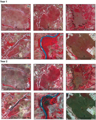
Figure 2. OLI/Landsat-8 false color composite (bands 5, 4 and 3 in RGB) from year 1 (19 June 2015) and year 2 (27 October 2016) showing examples of vegetation types found in the study area. (a) grassland (open grassland); (b) shrub savanna (open grassland with sparse shrubs); (c) woodland savanna (mixed grassland, shrublands and trees up to seven meters in height); (d) palm swaps (riparian vegetation); (e) semideciduous forest (semideciduous canopy foliage); and (f) deciduous forest (predominance of deciduous trees whose loss of foliage reaches more than 50%).

The climate is tropical with rainfall concentrated in October to May. The peak of the dry season in August has close to zero rainfall and air humidity less than 20% with high seasonality (Peel, Finlayson, and McMahon 2006). Rainfall in this region is extremely irregular over space and time. More than 75% of the total annual rainfall occurs within three months, but interannual variation in precipitation is large and droughts can last for years in areas of Caatinga (Leal et al. 2005).

3. Methodology

We developed a new OBCD method to detect human-induced changes in TSBs by reducing the effects of vegetation phenology on change detection, combining both the spatial and spectral domains of bi-temporal NDVI images. We used semivariogram indices (SIs) as spatial features (Balaguer et al. 2010), as described below (see Table 1). Descriptive statistics for NDVI imagery was used to represent spectral features (SFs), as detailed below (see section 3.4.).

Table 1. Semivariogram indices (SIs) calculated from the NDVI values inside the objects near the origin (*) or up to the first maximum (**). The semivariogram features {(h1, γ1), (h2, γ2) … (hn, γn)} are the points of the experimental semivariogram, as described by Balaguer et al. (2010). The lags {hi, h2 … hn} are equally spaced. Variance is the value of the total variance of the pixels belonging to the object. hmax_1 represents the location of the first local maximum, while γ(hmax_1) is the first local maximum semivariance.

Description	Formula
*Ratio between the values of the total variance and the semivariance at first lag	$\mathrm{R}\mathrm{V}\mathrm{F}=\frac{\mathrm{V}\mathrm{a}\mathrm{r}\mathrm{i}\mathrm{a}\mathrm{n}\mathrm{c}\mathrm{e}}{\gamma 1}$
*First derivative near the origin	$\mathrm{F}\mathrm{D}\mathrm{O}=\frac{\gamma 2-\gamma 1}{\mathrm{h}}$
*Second derivative at third lag	$\mathrm{S}\mathrm{D}\mathrm{T}=\frac{\gamma 4-2\gamma 3+\gamma 2}{{\mathrm{h}}^2}$
**Mean of the semivariogram values up to the first maximum	$\mathrm{M}\mathrm{F}\mathrm{M}=\frac{1}{\mathrm{M}\mathrm{a}\mathrm{x}\mathrm{\_}1}{\sum }^{\gamma \mathrm{i}}$
**Difference between the mean of the semivariogram values up to the first maximum and the semivariance at first lag	$\mathrm{D}\mathrm{M}\mathrm{F}=\mathrm{M}\mathrm{F}\mathrm{M}-\gamma \mathrm{i}$
**Semivariance curvature	$\mathrm{A}\mathrm{F}\mathrm{M}=\frac{\mathrm{h}}{2}\left(\gamma 1+2\left(\sum _{\mathrm{i}=2}^{\mathrm{m}\mathrm{a}\mathrm{x}\mathrm{\_}1-1}\gamma 1\right)+{\gamma }_{\mathrm{m}\mathrm{a}\mathrm{x}\mathrm{\_}1}\right)-\left(\gamma 1\left({\mathrm{h}}_{\mathrm{m}\mathrm{a}\mathrm{x}\mathrm{\_}1}-\mathrm{h}1\right)\right)$

By training MLAs using the difference between the two NDVI images in terms of spatial and spectral features, we were able to classify changes caused by phenology and those caused by human-induced disturbances. The method is summarized in six steps (Figure 3), which are described in detail in the following sections.

Figure 3. The six main steps in the methodology used to reduce the effects of seasonal NDVI changes caused by vegetation phenology on the detection of changes caused by human-induced disturbances in tropical seasonal biomes (TSBs) in Brazil.

3.1. Image acquisition

We used two cloud-free OLI/Landsat-8 images to calculate NDVI and test our method: one image was obtained on 19 June 2015 (Figure 4a) and the other was obtained on 27 October 2016 (Figure 4b). They were selected from the dry and rainy seasons to maximize the effects of vegetation seasonality. We used the image acquired in June 2015 as representative of the end of the rainy season with high NDVI values. On the other hand, the image acquired in October 2016 was used as representative of the end of the dry season with comparatively lower NDVI values due to water stress (Figure 4c). The images were downloaded from the United States Geological Survey (USGS) with geometric and atmospheric corrections. We used NDVI (Rouse et al. 1973) because the spatial domain of this index has been explored in several LULCC studies (Hamunyela, Verbesselt, and Herold 2016; Silveira et al. 2018a, 2018b). However, the proposed approach may be applied to any index.

Figure 4. (a) NDVI OLI/Landsat-8 image from 19 June 2015; (b) NDVI OLI/Landsat-8 image from 27 October 2016; (c) monthly precipitation pattern from years 2015, 2016 and historical series of precipitation from year 1952 to 2018.

3.2. Image segmentation

The first procedure in the OBCD method was image segmentation. We applied the multiresolution segmentation algorithm (Baatz and Schäpe 2000) from the eCognition software (Definies 2009) selecting the original bands of the OLI/Landsat-8 images acquired in 2015 and 2016 (years 1 and 2). This approach has the distinct advantage of considering all images during object formation, thus minimizing sliver errors and potentially honoring key multi-temporal boundaries (Desclée, Bogaert, and Defourny 2006; Tewkesbury et al. 2015). We used the following parameters: 0.1 for shape and 0.5 for compactness. The most critical step is the selection of the scale parameter (SP), which controls the size of the image objects. The SP sets a homogeneity threshold that determines the number of neighboring pixels that can be merged together to form an image object (Benz et al. 2004). The SP directly influences the size of the objects which are related to the predefined semivariogram criteria (lag distance) and the minimum number of pixels inside each object necessary to generate the semivariogram. We adopted a trial and error approach (Duro, Franklin, and Dube 2012) to find an appropriate value for SP (Chen et al. 2015). We ensured a minimum number of samples (25 pixels) inside the objects and an adequate size to allow calculation of the semivariogram. The SP (set to 250) and image segmentation results were assessed based on visual inspection of the delineated polygons (Figure 5). The objects generated were overlapped with the NDVI images from 2015 and 2016 to extract the input data for the OBCD method.

Figure 5. Image segmentation results using 0.1 for shape, 0.5 for compactness and 250 for the scale parameter (SP).

3.3. Class definition for change detection

This study focused on two broad classes: (i) vegetation covers with seasonal changes in NDVI caused by phenology (Figure 6a); and (ii) vegetation covers with changes caused by disturbances, especially human-induced deforestation/clearing (Figure 6b) and fires (Figure 6c). Historically, most of the fires detected in the area have been considered human-induced events. Therefore, we did not evaluate events of natural occurrence.

Figure 6. The location of the training and validation samples is shown at the top of the figure. The OLI/Landsat-8 false color composites (bands 5, 4 and 3 in RGB) show examples of the classes defined for change detection analysis between the rainy and dry seasons of 2015 (year 1) and 2016 (year 2). Seasonal variations caused by vegetation phenology are shown in (a), while human-induced changes caused by deforestation and fires are illustrated in (b) and (c), respectively.

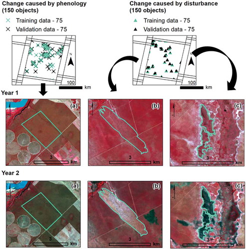
Representative areas of these two classes were identified from visual inspection of the images and from available land-cover maps. Randomly stratified design was used to sample these areas (Olofsson et al. 2014). We first used a land-cover map (Carvalho et al. 2006) showing the native vegetation for the 2006–2008 period to mask out the non-vegetated areas. Subsequently, we performed post-classification and image edition using a skilled human interpreter to update the available map to 2015 (Figure 1c). Thus, a dataset of 300 objects (well-distributed polygons over the vegetated areas; 150 per class) was obtained. The samples were randomly divided into training (50%) and validation (50%) datasets (Figure 6).

3.4. Feature extraction

We extracted spatial and spectral features based on the NDVI values inside the objects. The spatial information was obtained from experimental semivariograms (Equation (1)), where γ(h) is the estimator of the semivariance for each distance h, N (h) is the number of pairs of points (pixels) separated by distance h, Z(x) is the value of the regionalized variable at point x, and Z(x+ h) is the value at point (x+ h):

(1) $\hspace{0.17em}\gamma \left(\mathrm{h}\right)=\left(\frac{1}{2\mathrm{N}(\mathrm{h})}\right){\sum }_{\mathrm{i}=1}^{\mathrm{N}(\mathrm{h})}{\left(\mathrm{Z}\left(\mathrm{x}\right)-\mathrm{Z}\left(\mathrm{x}+\mathrm{h}\right)\right)}^2$(1)

Semivariance functions are characterized by three parameters: sill (σ²), range (φ) and nugget effect (τ²). The sill is the plateau reached by the semivariance values, measuring the variance explained by the spatial structure of the data. The range is the distance until the semivariogram reaches the sill, reflecting the distance at which the data become correlated. The nugget effect is the non-spatial component of the variance composed of random sensor noise or sampling errors (Curran 1988). We attempted to find an optimal lag distance to ensure that sill values would provide a concise description of data variability. We fixed the number of lags as 30 pixels and the lag size equivalent to the image spatial resolution (30 m), resulting in a lag distance of 900 m.

We extracted a set of semivariogram indices (SIs) (Balaguer et al. 2010) using the feature extraction software FETEX 2.0 for object-based image analysis (Ruiz et al. 2011) (Table 1). These indices describe the shape of the experimental semivariograms and, therefore, the properties that characterize the spatial patterns of the image objects. They have been categorized according to the position of the lags used in their definition: (i) near the origin and (ii) up to the first maximum.

As described by Balaguer et al. (2010), the ratio between the values of the total variance and the semivariance at first lag (RVF) is an indicator of the relationship between the spatial correlation at long and short distances. The first derivative near the origin (FDO) represents the slope of the semivariogram at the first two lags. The second derivative semivariogram at the third lag (SDT) quantifies the concavity or convexity level of the semivariogram at short distances, representing the heterogeneity of the objects in the image. The mean of the semivariogram values up to the first maximum (MFM) is an indicator of the average of the semivariogram values between the first lag and the first maximum. It provides information about the changes in the data variability and is related to the concavity or convexity of the semivariogram in that interval. The difference between the mean of the semivariogram values up to the first maximum (MFM) and the semivariance at first lag shows the decreasing rate of the spatial correlation in the image up to the lags where the semivariogram theoretically tends to be stabilized. Finally, the area between the semivariogram value in the first lag and the semivariogram function until the first maximum (AFM) provides information about the semivariogram curvature, which is also related to the variability of the data.

To explore the spectral information of the satellite images, we used the minimum (MIN), mean (MEAN), maximum (MAX) and standard deviation (STDEV) of the NDVI values inside each object. This allowed the performance of spatial and spectral features to be compared and combined.

3.5. Change detection using MLAs

After extracting the spatial and spectral features for each object, the differences in NDVI values for each feature between years 1 (2015) and 2 (2016) were calculated and used as input data to train the MLAs. The samples were randomly divided into training (50%) and validation (50%) datasets. We used three MLAs implemented in the Waikato Environment for Knowledge Analysis (WEKA 3.8 software): SVM, ANN and RF.

SVM has the ability to handle small training datasets, often producing higher classification accuracies than traditional methods (Bovolo, Camps-Valls, and Bruzzone 2010; Mantero, Moser, and Serpico 2005; Wyle et al. 2018). For SVM, we used the radial basis function (RBF) kernel, as this is known to be effective and accurate (Pereira et al. 2017; Shao and Lunetta 2012; Zuo, John, and Carranza 2011; Wu et al. 2015). To train the SVM classifier, an error parameter C (10) and a kernel parameter γ (0.1) were set after a series of tests and analyses of the outputs.

There are many different types of ANN, but the multilayer perceptron (MLP) is most commonly used in remote sensing (Berberoglu et al. 2000; Vafaei et al. 2018; Zhang et al. 2018). We used the ANN obtained by running the MLP function with the back-propagation algorithm (Pham, Yoshino, and Tien Bui 2017). The main challenge associated with MLP is the adjustment of network parameters (Shao and Lunetta 2012). The learning rate, the momentum term, and iteration numbers were fixed at 0.3, 0.2 and 500, respectively (Tien Bui et al. 2016).

We also tested the non-parametric RF algorithm (Breiman 2001) because it has the ability to accommodate many predictor variables with accuracy and efficiency (Breiman 2001; DeVries et al. 2016; Ghimire, Rogan, and Miller 2010; Silveira et al. 2018a; Zhu et al. 2016). We set the number of decision trees (Ntree), to 500 (Lawrence, Shana, and Sheley 2006) and the number of variables for the best split when growing the trees (Mtry) to the default value (log of the number of features + 1) (Millard and Richardson 2015).

3.6. Change detection evaluation

To evaluate our change detection using the three MLAs, we tested: (i) the spatial domain of the NDVI images using the SIs; (ii) the spectral domain of the NDVI images using the SFs; and (iii) the combination of the spatial-spectral attributes (SIs plus SFs). We obtained a confusion matrix to evaluate classification accuracy for the two classes under analysis: (a) vegetation covers with seasonal changes in NDVI caused by phenology; and (b) vegetation covers with NDVI changes caused by human-induced disturbances. We evaluated the overall, producer’s and user’s accuracies.

4. Results

4.1. Semivariogram analysis

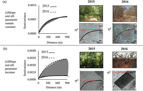
From the use of semivariograms to quantify the spatial variability of the NDVI pixels inside the objects, we found the maximum level of semivariance (sill – σ² semivariogram parameter) at around 900 m. This indicated that at least 30 pixels and a lag size equivalent to the image spatial resolution (30 m) were necessary to quantify spatial variability of the OLI/Landsat-8 images. We detected two distinct patterns in the semivariograms: (i) the shape and the overall data variability (sill – σ²) remained constant over time with seasonal changes in NDVI caused by phenology (Figure 7a); and (ii) the shape and sill increased in areas that experienced human-induced disturbances between 2015 and 2016 (Figure 7b). These results indicated that the spatial variability of NDVI quantified by semivariograms was very sensitive to changes in vegetation cover caused by deforestation or fires. On the other hand, seasonal changes in NDVI caused by vegetation phenology did not modify the shape and overall variability of the semivariograms.

Figure 7. Patterns of semivariograms generated from the NDVI values inside the objects for years 1 (2015) and 2 (2016): (a) NDVI changes caused by vegetation phenology – the shape and sill (σ²) parameters remained constant; (b) NDVI changes caused by human-induced disturbances – the shape and sill (σ²) parameters increased.

4.2. Change detection evaluation

When we used the MLAs to classify areas with seasonal NDVI variations caused by vegetation phenology and areas with NDVI variations caused by human-induced disturbances, our results showed overall classification accuracies higher than 80% for SVM, ANN and RF considering the spectral features and semivariogram indices (Table 2). Therefore, these classifiers and features were generally efficient to discriminate areas of vegetation covers with seasonal changes in NDVI caused by phenology from other disturbance-affected areas.

Table 2. Confusion matrix from the classification of areas with seasonal NDVI changes caused by vegetation phenology and those due to human-induced disturbances. Spectral features (SFs), semivariogram indices (SIs) and their combination (SFs + SIs) were used for change detection. The Producer’s (PA), User’s (UA) and overall (OA) classification accuracies are shown for support vector machine (SVM), artificial neural network (ANN) and random forest (RF).

	Vegetation change class	SF		SI		SF + SI
		PA (%)	UA (%)	PA (%)	UA (%)	PA (%)	UA (%)
SVM	Change caused by disturbance	88.76	79.00	94.05	79.00	94.68	90
	Change caused by phenology	82.20	90.65	82.93	95.33	90.27	95.33
	OA (%)	85.02		87.43		92.27
ANN	Change caused by disturbance	87.21	75.00	88.24	75.00	93.55	87.00
	Change caused by phenology	79.34	89.72	79.51	90.65	88.60	94.39
	OA (%)	82.6		83.09		90.82
RF	Change caused by disturbance	84.54	82.00	87.37	83.00	91.84	90.00
	Change caused by phenology	83.64	85.98	84.82	88.79	90.83	92.52
	OA (%)	84.05		85.99		91.3

The classification results using SFs (MIN, MEAN, MAX and STDEV) produced the lowest accuracies, reaching values of 85.02%, 82.60% and 84.05% for SVM, ANN and RF, respectively. The lowest user’s and producer’s accuracies were obtained using this group of features (Table 2). In contrast, the overall classification accuracies slightly improved when the semivariogram indices (RVF, FDO, SDT, MFM, DMF and AFM) were included in the analysis, producing values of 87.43%, 83.09% and 85.99% for SVM, ANN and RF, respectively. Thus, the semivariogram indices performance slightly better than the spectral features, because they are related to the structured variance of the NDVI pixel values.

A substantial gain in classification accuracy, reducing confusion between vegetation phenological changes and human-induced disturbances, was obtained from the combination of the SIs and the SFs (Table 2). The accuracies increased from 85.02 to 92.27%, 82.60 to 90.82% and 84.05 to 91.30% for SVM, ANN and RF, respectively. The highest user’s accuracy, considering both groups of features and all MLAs, was observed for the class with changes controlled by vegetation phenology (95.33%). The user’s accuracies for this class improved significantly from 90.65 to 95.33% (SVM), 89.72 to 94.39 (ANN) and from 85.98 to 92.52% (RF). This was highly significant because the objects with seasonal changes in NDVI presented low commission errors. On the other hand, the highest producer’s accuracy was observed for the class with changes caused by human-induced disturbances having 94.68% for the SVM classifier.

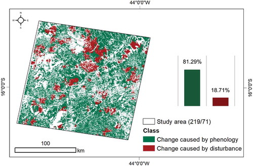
The classification performance of the MLAs was generally comparable, but the SVM algorithm was the most effective classifier in our TSBs. In Table 2, the SVM presented the highest overall classification accuracy (92.27%). Using SFs or SIs as well as the combination of these features, the accuracies were slightly superior for SVM than for ANN and RF. The differences in performance are probably due to the difficulties of parameterization between the MLAs (García-Gutiérrez et al. 2015). SVM have been frequently cited as a group of theoretically superior machine learning algorithms for image classification and have been shown to perform well (Foody and Mathur 2004). They appear to be especially advantageous in the presence of heterogeneous classes for which only a few training samples are available (Li, Im, and Beier 2013; Wu et al. 2015). The resultant SVM classification map, using the hybrid set of spatial and spectral features from the OLI/Landsat-8 data, is shown in Figure 8. From the vegetated areas, 18.71% of changes (331,830 ha) were caused by human-induced disturbances between 2015 and 2016.

Figure 8. Support vector machine (SVM) classification using spectral features (SFs) and semivariogram indices (SIs), showing changes caused by vegetation phenology and human-induced disturbance between 2015 and 2016.

5. Discussion

5.1. Remote sensing change detection in TSBs

We proposed a new object-based method to detect changes caused by either vegetation phenology or human-induced disturbances in TSBs, based on the differences over time in spatial (semivariogram indices) and spectral features (descriptive statistics for NDVI). Spatial and spectral features were used to train MLAs (SVM, ANN and RF). Our results showed that the combination of both group of features produced the highest overall classification, producer’s and user’s accuracies.

The method is an alternative to detect changes in TSBs, because it does not require high-quality time series, which are sometimes difficult to obtain due to cloud cover. This method could be used to improve the accuracy of LULCC maps, thus providing better inputs for the assessment of atmospheric emissions derived from deforestation and fires (Mouillot et al. 2014). TSBs present a conspicuous seasonal contrast between the rainy and dry seasons (Ferreira and Huete 2004), which is challenging for change detection. The seasonality of TSBs makes the use of optical remote sensing difficult in some periods of the years due to cloud-cover and vegetation phenology. Most of the change detection algorithms that are based on two dates of Landsat images may reduce the influence of vegetation phenology on the analysis by fixing data acquisition to a given period (Lu et al. 2004; Zhu, Woodcock, and Olofsson 2012). However, in TSBs in eastern Brazil, even fixing a pair of dates to the rainy or dry season, the confounding effects of vegetation phenology on change detection persist because of the irregular patterns of precipitation observed over space and time.

Some remote sensing studies have mapped deforestation and fire in TSBs (Achard et al. 2014; Beuchle et al. 2015; Libonati et al. 2015; Hansen et al. 2013). For example, Beuchle et al. (2015) provided information on historical and recent vegetation cover changes in the Cerrado from central Brazil and the Caatinga from northeastern Brazil based on the analysis of Landsat images from 1990 to 2010. For the Cerrado, they estimated that 117,870 km² of vegetation was lost during the studied period, while for the Caatinga they reported a loss of 25,335 km². When these results were compared to LULCC estimates provided by other projects, such as the Conservation and Sustainable Use of Brazilian Biological Diversity Project (PROBIO) and Deforestation Monitoring in Brazilian Biomes Project (PMDBBS), some divergences were observed (Beuchle et al. 2015). Although there were several factors that could introduce differences in these estimates (e.g., spatial resolution, class definition), our findings showed that the confounding effects of vegetation phenology on change detection should be further considered as an important factor to avoid overestimation of human-induced disturbances.

5.2. Classification and change detection using the spatial-spectral domains of NDVI

The spatial domain has been recently used to detect changes in tropical regions. The phenological influence on data analysis is reduced when NDVI values are spatially normalized in a pixel-based change detection approach (Hamunyela, Verbesselt, and Herold 2016). The influence is also reduced when geostatistical features (spatial domain) are incorporated into the analysis of bi-temporal NDVI images in an object-based change detection approach (Silveira et al. 2018b). Although the integration between remote sensing and geostatistical theory was consolidated in the late 1980s, only recent studies have demonstrated that the semivariogram (a geostatistical tool) has strong potential for LULCC detection (Acerbi Junior et al. 2015; Gil-Yepes et al. 2016; Silveira et al. 2018a, 2018b).

Our study has demonstrated that the combination of spectral features and semivariogram indices derived from bi-temporal NDVI images reduced the effects of vegetation phenology on vegetation change detection. Misclassifications of seasonal NDVI changes caused by vegetation phenology as those caused by human-induced disturbances were therefore reduced. We found that LULCC areas caused by deforestation or fires provided singular semivariograms with higher values for the sill parameter than ones associated with vegetation phenology in savannas and semi-arid woodlands. These results are in agreement with several previous studies that used spatial information to detect changes (e.g. Acerbi Junior et al. 2015; Sertel, Kaya, and Curran 2007; Silveira et al. 2018a, 2018b).

Acerbi Junior et al. (2015) analyzed the potential of semivariograms generated from NDVI values to detect changes in Brazilian savannas. Their results showed a very clear trend, where the shape of semivariograms, and the sill and range parameters were different when deforestation occurred and were similar when there was no change in land cover, which was consistent with our findings. Silveira et al. (2018a), (2018b)) highlight the importance of considering spatial information for change detection in Brazilian savannas in the absence of a dense time series of remote-sensing images. When using individual spatial features (e.g. sill parameter and the AFM index) the change detection results were improved considerably compared with the spectral features and image differencing technique. These results demonstrated that the semivariograms derived from NDVI images are not affected by phenological changes.

Here, by including SIs that provided information near the origin (RVF, FDO and SDT) and up to the first maximum (MFM, DMF and AFM), we obtained sufficient separability between the classes of vegetation changes caused by phenology and human-induced disturbances. By combining SIs with SFs, the misclassification of these two classes was reduced, as expressed by overall classification accuracies close to 90% for the three classifiers (SVM, ANN and RF) (Table 2).

6. Conclusions

We have proposed a new OBCD method to detect and distinguish vegetation changes caused by phenology from those caused by human-induced disturbances in Brazilian TSBs with pronounced seasonality. We reduced the effects of vegetation phenology on change detection by combining features from both the spatial and spectral domains of NDVI satellite images. The spatial variability of NDVI is not affect by vegetation seasonality, favoring the addition of semivariogram indices to reduce the impact of seasonality for detecting deforestation or fires using bi-temporal Landsat images.

Compared with the other classifiers tested with this method, SVM presented a slightly higher overall classification accuracy (92.27%) when using the hybrid set of NDVI-derived spectral and spatial features. Finally, our study highlights that the combination of the spatial and spectral attributes reduces the requirement for dense time series of satellite imagery throughout multiple phenological cycles to detect LULCC in TSBs. In these areas, vegetation exhibits strong seasonality and regularly-spaced satellite images are difficult to obtain due to persistent cloud-cover. Future studies should aim to evaluate further the proposed method, including its sensitivity to class and intensity of disturbance, and its applicability to other TSBs.

Acknowledgements

The authors would like to thank the Coordenação de Aperfeiçoamento de Pessoal de Nível Superior - Brasil (CAPES) for financing part of this study (Finance Code 001). The authors are grateful for comments and suggestions by the anonymous reviewers.

Disclosure statement

No potential conflict of interest was reported by the authors.

References

- Acerbi Junior, F. W., E. M. O. Silveira, J. M. Mello, C. R. Mello, and J. R. S. Scolforo. 2015. “Change Detection in Brazilian Savannas Using Semivariograms Derived from NDVI Images.” Ciência e Agrotecnologia 39 (2): 103–109. doi:10.1590/S1413-70542015000200001.
- Achard, F., R. Beuchle, P. Mayaux, H. J. Stibig, C. Bodart, A. Brink, S. Carboni, et al. 2014. “Determination of Tropical Deforestation Rates and Related Carbon Losses from 1990 to 2010.” Global Change Biology 20 (8): 2540–2554. doi:10.1111/gcb.12605.
- Baatz, M., and A. Schäpe. 2000. “Multiresolution Segmentation : An Optimization Approach for High Quality Multi-Scale Image Segmentation.” Journal of Photogrammetry and Remote Sensing 58 (3–4): 12–23.
- Balaguer, A., L. A. Ruiz, T. Hermosilla, and J. A. Recio. 2010. “Definition of a Comprehensive Set of Texture Semivariogram Features and Their Evaluation for Object-Oriented Image Classification.” Computers and Geosciences 36 (2): 231–240. doi:10.1016/j.cageo.2009.05.003.
- Benz, U. C., P. Hofmann, G. Willhauck, I. Lingenfelder, and M. Heynen. 2004. “Multi-Resolution, Object-Oriented Fuzzy Analysis of Remote Sensing Data for GIS-Ready Information.” ISPRS Journal of Photogrammetry and Remote Sensing 58 (3–4): 239–258. doi:10.1016/j.isprsjprs.2003.10.002.
- Berberoglu, S., C. D. Lloyd, P. M. Atkinson, and P. J. Curran. 2000. “The Integration of Spectral and Textural Information Using Neural Networks for Land Cover Mapping in the Mediterranean.” Computers and Geosciences 26 (4): 385–396. doi:10.1016/S0098-3004(99)00119-3.
- Beuchle, R., R. C. Grecchi, Y. E. Shimabukuro, R. Seliger, H. D. Eva, E. Sano, and F. Achard. 2015. “Land Cover Changes in the Brazilian Cerrado and Caatinga Biomes from 1990 to 2010 Based on a Systematic Remote Sensing Sampling Approach.” Applied Geography 58: 116–127. doi:10.1016/j.apgeog.2015.01.017.
- Bovolo, F., G. Camps-Valls, and L. Bruzzone. 2010. “A Support Vector Domain Method for Change Detection in Multitemporal Images.” Pattern Recognition Letters 31 (10): 1148–1154. doi:10.1016/j.patrec.2009.07.002.
- Breiman, L. 2001. “Random Forests.” Machine Learning 45 (1): 5–32. doi:10.1023/A:1010933404324.
- Carvalho, L. M. T., J. R. S. Scolforo, A. D. Oliveira, J. M. Mello, L. T. Oliveira, F. W. Acerbi Junior, H. C. Cavalcanti, and R. Vargas Filho. 2006. “Procedimentos de Mapeamento.” In: Mapeamento e Inventário da Flora e dos Reflorestamentos de Minas Gerais, 37–57. Lavras: UFLA.
- Chen, G., G. J. Hay, L. M. T. Carvalho, and M. A. Wulder. 2012. “Object-Based Change Detection.” International Journal of Remote Sensing 33 (14): 4434–4457. doi:10.1127/1432-8364/2011/0085.
- Chen, G., Q. Weng, G. J. Hay, and Y. He. 2018. “Geographic Object-Based Image Analysis (GEOBIA): Emerging Trends and Future Opportunities.” GIScience & Remote Sensing 55 (2): 159–182. doi:10.1080/15481603.2018.1426092.
- Chen, X., D. Yang, J. Chen, and X. Cao. 2015. “An Improved Automated Land Cover Updating Approach by Integrating with Downscaled NDVI Time Series Data.” Remote Sensing Letters 6 (1): 29–38. doi:10.1080/2150704X.2014.998793.
- Curran, P. J. 1988. “The Semivariogram in Remote Sensing: An Introduction.” Remote Sensing of Environment 24 (3): 493–507. doi:10.1016/0034-4257(88)90021-1.
- Definies, A. G. 2009. Definiens ECognition Developer 8 User Guide. Munchen, Germany: Definens AG.
- Desclée, B., P. Bogaert, and P. Defourny. 2006. “Forest Change Detection by Statistical Object-Based Method.” Remote Sensing of Environment 102 (1–2): 1–11. doi:10.1016/j.rse.2006.01.013.
- DeVries, B., A. K. Pratihast, J. Verbesselt, L. Kooistra, and M. Herold. 2016. “Characterizing Forest Change Using Community-Based Monitoring Data and Landsat Time Series.” PLoS ONE 11 (3): 1–25. doi:10.1371/journal.pone.0147121.
- Duro, D. C., S. E. Franklin, and M. G. Dube. 2012. “A Comparison of Pixel-Based and Object-Based Image Analysis with Selected Machine Learning Algorithms for the Classification of Agricultural Landscapes Using SPOT-5 HRG Imagery.” Remote Sensing of Environment 118: 259–272. doi:10.1016/j.rse.2011.11.020.
- Espírito-Santo, M. M., M. E. Leite., J. O. Silva, R. S. Barbosa, A. M. Rocha, F. C. Anaya, and M. G. V. Dupin. 2016. “Understanding Patterns of Land-Cover Change in the Brazilian Cerrado from 2000 to 2015.” Philosophical Transactions of the Royal Society B Biological Sciences, no. 371: 1–11. doi:10.1098/rstb.2015.0435.
- Evans, J., and R. Geerken. 2004. “Discrimination between Climate and Human-Induced Dryland Degradation.” Journal of Arid Environments 57: 535–554. doi:10.1016/S0140-1963(03)00121-6.
- Ferreira, L. G., and A. R. Huete. 2004. “Assessing the Seasonal Dynamics of the Brazilian Cerrado Vegetation through the Use of Spectral Vegetation Indices.” International Journal of Remote Sensing 25 (10): 1837–1860. doi:10.1080/0143116031000101530.
- Ferreira, L. G., H. Yoshioka, A. Huete, and E. E. Sano. 2004. “Optical Characterization of the Brazilian Savanna Physiognomies for Improved Land Cover Monitoring of the Cerrado Biome: Preliminary Assessments from an Airborne Campaign over an LBA Core Site.” Journal of Arid Environments 56 (3): 425–447. doi:10.1016/S0140-1963(03)00068-5.
- Foody, G. M., and A. Mathur. 2004. “A Relative Evaluation of Multiclass Image Classification by Support Vector Machines.” IEEE Transactions on Geoscience and Remote Sensing 42 (6): 1335–1343. doi:10.1109/TGRS.2004.827257.
- García-Gutiérrez, J., D. Mateos-García, M. Garcia, and J. C. Riquelme-Santos. 2015. “An Evolutionary-Weighted Majority Voting and Support Vector Machines Applied to Contextual Classification of LiDAR and Imagery Data Fusion.” Neurocomputing 163: 17–24. doi:10.1016/j.neucom.2014.08.086.
- Ghimire, B., J. Rogan, and J. Miller. 2010. “Contextual Land-Cover Classification: Incorporating Spatial Dependence in Land-Cover Classification Models Using Random Forests and the Getis Statistic.” Remote Sensing Letters 1 (1): 45–54. doi:10.1080/01431160903252327.
- Gil-Yepes, J. L., L. A. Ruiz, J. A. Recio, A. Balaguer-Beser, and T. Hermosilla. 2016. “Description and Validation of a New Set of Object-Based Temporal Geostatistical Features for Land-Use/Land-Cover Change Detection.” ISPRS Journal of Photogrammetry and Remote Sensing 121: 77–91. doi:10.1016/j.isprsjprs.2016.08.010.
- Hamunyela, E., J. Reiche, J. Verbesselt, and M. Herold. 2017. “Using Space-Time Features to Improve Detection of Forest Disturbances from Landsat Time Series.” Remote Sensing 9 (6): 1–17. doi:10.3390/rs9060515.
- Hamunyela, E., J. Verbesselt, and M. Herold. 2016. “Using Spatial Context to Improve Early Detection of Deforestation from Landsat Time Series.” Remote Sensing of Environment 172: 126–138. doi:10.1016/j.rse.2015.11.006.
- Hansen, M. C., P. V. Potapov, R. Moore, M. Hancher, S. A. Turubanova, A. Tyukavina, D. Thau, et al. 2013. “High-Resolution Global Maps of 21st-Century Forest Cover Change.” Science 342 (6160): 850–853. doi:10.1126/science.1244693.
- Healey, S. P., W. B. Cohen, Z. Yang, C. K. Brewer, E. B. Brooks, N. Gorelick, A. J. Hernandez, et al. 2018. “Mapping Forest Change Using Stacked Generalization: An Ensemble Approach.” Remote Sensing of Environment 204: 717–728. doi:10.1016/j.rse.2017.09.029.
- Hoekstra, J. M., T. M. Boucher, T. H. Ricketts, and C. Roberts. 2005. “Confronting a Biome Crisis: Global Disparities of Habitat Loss and Protection.” Ecology Letters 8 (1): 23–29. doi:10.1111/j.1461-0248.2004.00686.x.
- Huang, C., S. N. Goward, J. G. Masek, N. Thomas, Z. Zhu, and J. E. Vogelmann. 2010. “Remote Sensing of Environment an Automated Approach for Reconstructing Recent Forest Disturbance History Using Dense Landsat Time Series Stacks.” Remote Sensing of Environment 114 (1): 183–198. doi:10.1016/j.rse.2009.08.017.
- Hughes, M. J., S. D. Kaylor, and D. J. Hayes. 2017. “Patch-Based Forest Change Detection from Landsat Time Series.” Forests 8 (5): 1–22. doi:10.3390/f8050166.
- Ibrahim, Y. Z., H. Balzter, J. Kaduk, and C. J. Tucker. 2015. “Land Degradation Assessment Using Residual Trend Analysis of GIMMS NDVI3g, Soil Moisture and Rainfall in Sub-Saharan West Africa from 1982 to 2012.” Remote Sensing 7: 5471–5494. doi:10.3390/rs70505471.
- Kennedy, R. E., Z. Yang, and W. B. Cohen. 2010. “Remote Sensing of Environment Detecting Trends in Forest Disturbance and Recovery Using Yearly Landsat Time Series : 1. LandTrendr — Temporal Segmentation Algorithms.” Remote Sensing of Environment 114 (12): 2897–2910. doi:10.1016/j.rse.2010.07.008.
- Lagomasino, D., R. M. Price, D. Whitman, P. K. E. Campbell, and A. Melesse. 2014. “Estimating Major Ion and Nutrient Concentrations in Mangrove Estuaries in Everglades National Park Using Leaf and Satellite Reflectance.” Remote Sensing of Environment 154: 202–218. doi:10.1016/j.rse.2014.08.022.
- Laliberte, A. S., and A. Rango. 2009. “Texture and Scale in Object-Based Analysis of Subdecimeter Resolution Unmanned Aerial Vehicle (UAV) Imagery.” IEEE Transactions on Geoscience and Remote Sensing 47 (3): 761–770. doi:10.1109/TGRS.2008.2009355.
- Lawrence, R. L., D. W. Shana, and R. L. Sheley. 2006. “Mapping Invasive Plants Using Hyperspectral Imagery and Breiman Cutler Classifications (Randomforest).” Remote Sensing of Environment 100 (3): 356–362. doi:10.1016/j.rse.2005.10.014.
- Leal, I. R., J. M. C. Silva, M. Tabarelli, and T. E. Lacher. 2005. “Changing the Course of Biodiversity Conservation in the Caatinga of Northeastern Brazil.” Conservation Biology 19 (3): 701–706. doi:10.1111/j.1523-1739.2005.00703.x.
- Li, M., J. Im, and C. Beier. 2013. “Machine Learning Approaches for Forest Classification and Change Analysis Using Multi-Temporal Landsat TM Images over Huntington Wildlife Forest.” Giscience & Remote Sensing 50 (4): 361–384. doi:10.1080/15481603.2013.819161.
- Libonati, R., C. C. Camara, A. W. Setzer, F. Morelli, and A. E. Melchiori. 2015. “An Algorithm for Burned Area Detection in the Brazilian Cerrado Using 4 Μm MODIS Imagery.” Remote Sensing 7 (11): 15782–15803. doi:10.3390/rs71115782.
- Lu, D., P. Mausel, E. Brondízio, and E. Moran. 2004. “Change Detection Techniques.” International Journal of Remote Sensing 25 (12): 2365–2401. doi:10.1080/0143116031000139863.
- Mantero, P., G. Moser, and S. B. Serpico. 2005. “Partially Supervised Classification of Remote Sensing Images through SVM-Based Probability Density Estimation.” IEEE Transactions on Geoscience and Remote Sensing 43 (3): 559–570. doi:10.1109/TGRS.2004.842022.
- Millard, K., and M. Richardson. 2015. “On the Importance of Training Data Sample Selection in Random Forest Image Classification: A Case Study in Peatland Ecosystem Mapping.” Remote Sensing 7 (7): 8489–8515. doi:10.3390/rs70708489.
- Mouillot, F., M. G. Schultz, C. Yue, P. Cadule, K. Tansey, P. Ciais, and E. Chuvieco. 2014. “Ten Years of Global Burned Area Products from Spaceborne Remote Sensing-A Review: Analysis of User Needs and Recommendations for Future Developments.” International Journal of Applied Earth Observation and Geoinformation 26 (1): 64–79. doi:10.1016/j.jag.2013.05.014.
- Olofsson, P., G. M. Foody, M. Herold, S. V. Stehman, C. E. Woodcock, and M. A. Wulder. 2014. “Good Practices for Estimating Area and Assessing Accuracy of Land Change.” Remote Sensing of Environment 148: 42–57. doi:10.1016/j.rse.2014.02.015.
- Peel, M. C., B. L. Finlayson, and T. A. McMahon. 2006. “Updated World Map of the K ̈Oppen-Geiger Climate Classification.” Meteorologische Zeitschrift 15: 259–263. doi:10.1127/0941-2948/2006/0130.
- Pereira, A. A., J. M. C. Pereira, R. Libonati, D. Oom, A. W. Setzer, F. Morelli, F. Machado-Silva, and L. M. T. Carvalho. 2017. “Burned Area Mapping in the Brazilian Savanna Using a One-Class Support Vector Machine Trained by Active Fires.” Remote Sensing 9 (11): 1161. doi:10.3390/rs9111161.
- Pham, T. D., K. Yoshino, and D. Tien Bui. 2017. “Biomass Estimation of Sonneratia Caseolaris (L.) Engler at a Coastal Area of Hai Phong City (Vietnam) Using ALOS-2 PALSAR Imagery and GIS-Based Multi-Layer Perceptron Neural Networks.” GIScience and Remote Sensing 54 (3): 329–353. doi:10.1080/15481603.2016.1269869.
- Rouse, J. W., R. H. Hass, J. A. Schell, and D. W. Deering. 1973. “Monitoring Vegetation Systems in the Great Plains with ERTS.” Third Earth Resources Technology Satellite (ERTS) Symposium 1: 309–317.
- Ruiz, L. A., J. A. Recio, A. Fernández-Sarría, and T. Hermosilla. 2011. “A Feature Extraction Software Tool for Agricultural Object-Based Image Analysis.” Computers and Electronics in Agriculture 76 (2): 284–296. doi:10.1016/j.compag.2011.02.007.
- Sano, E. E., R. Rosa, J. L. Brito, and L. G. Ferreira. 2010. “Land Cover Mapping of the Tropical Savanna Region in Brazil.” Environmental Monitoring and Assessment 166: 113–124. doi:10.1007/s10661-009-0988-4.
- Santos, R. M., A. T. Oliveira-Filho, P. V. Eisenlohr, L. P. Queiroz, D. B. O. S. Cardoso, and M. J. N. Rodal. 2012. “Identity and Relationships of the Arboreal Caatinga among Other Floristic Units of Seasonally Dry Tropical Forests (SDTFs) of North-Eastern and Central Brazil.” Ecology and Evolution 2 (2): 409–428. doi:10.1002/ece3.91.
- Scolforo, H. F., J. R. S. Scolforo, C. R. Mello, J. M. Mello, and A. C. Ferraz Filho. 2015. “Spatial Distribution of Aboveground Carbon Stock of the Arboreal Vegetation in Brazilian Biomes of Savanna, Atlantic Forest and Semi-Arid Woodland.” PLoS ONE 10 (6): 1–20. doi:10.1371/journal.pone.0128781.
- Sertel, E., S. Kaya, and P. J. Curran. 2007. “Use of Semivariograms to Identify Earthquake Damage in an Urban Area.” IEEE Transactions on Geoscience and Remote Sensing 45 (6): 1590–1594. doi:10.1109/TGRS.2007.894019.
- Shao, Y., and R. S. Lunetta. 2012. “Comparison of Support Vector Machine, Neural Network, and CART Algorithms for the Land-Cover Classification Using Limited Training Data Points.” ISPRS Journal of Photogrammetry and Remote Sensing 70: 78–87. doi:10.1016/j.isprsjprs.2012.04.001.
- Silva, J. F., M. R. Fariñas, J. M. Felfili, and C. A. Klink. 2006. “Spatial Heterogeneity, Land Use and Conservation in the Cerrado Region of Brazil.” Journal of Biogeography 33 (3): 536–548. doi:10.1111/j.1365-2699.2005.01422.x.
- Silveira, E. M. O., I. T. Bueno, F. W. Acerbi Júnior, J. M. Mello, J. R. S. Scolforo, and M. A. Wulder. 2018a. “Using Spatial Features to Reduce the Impact of Seasonality for Detecting Tropical Forest Changes from Landsat Time Series.” Remote Sensing 10 (6): 808–821. doi:10.3390/rs10060808.
- Silveira, E. M. O., J. M. Mello, F. W. Acerbi Júnior, and L. M. T. Carvalho. 2018b. “Object-Based Land-Cover Change Detection Applied to Brazilian Seasonal Savannahs Using Geostatistical Features.” International Journal of Remote Sensing 39 (8): 2597–2619. doi:10.1080/01431161.2018.1430397.
- Silveira, E. M. O., M. D. Menezes, F. W. Acerbi Júnior, M. C. N. S. Terra, and J. M. Mello. 2017. “Assessment of Geostatistical Features for Object-Based Image Classification of Contrasted Landscape Vegetation Cover.” Journal of Applied Remote Sensing 11 (3): 1–15. doi:10.1117/1.JRS.11.036004.
- Tewkesbury, A. P., A. J. Comber, N. J. Tate, A. Lamb, and P. F. Fisher. 2015. “A Critical Synthesis of Remotely Sensed Optical Image Change Detection Techniques.” Remote Sensing of Environment 160: 1–14. doi:10.1016/j.rse.2015.01.006.
- Tien Bui, D., T. A. Tuan, H. Klempe, B. Pradhan, and I. Revhaug. 2016. “Spatial Prediction Models for Shallow Landslide Hazards: A Comparative Assessment of the Efficacy of Support Vector Machines, Artificial Neural Networks, Kernel Logistic Regression, and Logistic Model Tree.” Landslides 13 (2): 361–378. doi:10.1007/s10346-015-0557-6.
- Vafaei, S., J. Soosani, K. Adeli, H. Fadaei, H. Naghavi, T. D. Pham, and D. Tien Bui. 2018. “Improving Accuracy Estimation of Forest Aboveground Biomass Based on Incorporation of ALOS-2 PALSAR-2 and Sentinel-2A Imagery and Machine Learning: A Case Study of the Hyrcanian Forest Area (Iran).” Remote Sensing 10 (2): 1–21. doi:10.3390/rs10020172.
- Verbesselt, J., R. Hyndman, G. Newnham, and D. Culvenor. 2010. “Detecting Trend and Seasonal Changes in Satellite Image Time Series.” Remote Sensing of Environment 114 (1): 106–115. doi:10.1016/j.rse.2009.08.014.
- Wright, S. J., and C. P. Van Schaik. 1994. “Light and the Phenology of Tropical Trees.” The American Naturalist 143 (1): 192–199. doi:10.1086/285600.
- Wu, X., J. Peng, J. Shan, and W. Cui. 2015. “Evaluation of Semivariogram Features for Object-Based Image Classification.” Geo-Spatial Information Science 18 (4): 159–170. doi:10.1080/10095020.2015.1116206.
- Wyle, B. K., N. J. Pastick, J. J. Picote, and C. A. Deering. 2018. “Geospatial Data Mining for Digital Raster Mapping.” GIScience & Remote Sensing 1–24. doi:10.1080/15481603.2018.1517445.
- Zhang, C., X. Pan, H. Li, A. Gardiner, I. Sargent, J. Hare, and P. M. Atkinson. 2018. “A Hybrid MLP-CNN Classifier for Very Fine Resolution Remotely Sensed Image Classification.” ISPRS Journal of Photogrammetry and Remote Sensing 140: 133–144. doi:10.1016/j.isprsjprs.2017.07.014.
- Zhang, K., M. Ross, and D. Gann. 2016. “Remote Sensing of Seasonal Changes and Disturbances in Mangrove Forest : A Case Study from South Florida.” Ecosphere 7: 1–23. doi:10.1002/ecs2.1366.
- Zhu, Z. 2017. “Change Detection Using Landsat Time Series : A Review of Frequencies, Preprocessing, Algorithms, and Applications.” ISPRS Journal of Photogrammetry and Remote Sensing 130: 370–384. doi:10.1016/j.isprsjprs.2017.06.013.
- Zhu, Z., Y. Fu, C. E. Woodcock, P. Olofsson, J. E. Vogelmann, C. Holden, M. Wang, S. Dai, and Y. Yu. 2016. “Including Land Cover Change in Analysis of Greenness Trends Using All Available Landsat 5, 7, and 8 Images: A Case Study from Guangzhou, China (2000–2014).” Remote Sensing of Environment 185: 243–257. doi:10.1016/j.rse.2016.03.036.
- Zhu, Z., and C. E. Woodcock. 2014. “Continuous Change Detection and Classification of Land Cover Using All Available Landsat Data.” Remote Sensing of Environment 144: 152–171. doi:10.1016/j.rse.2014.01.011.
- Zhu, Z., C. E. Woodcock, and P. Olofsson. 2012. “Continuous Monitoring of Forest Disturbance Using All Available Landsat Imagery.” Remote Sensing of Environment 122: 75–91. doi:10.1016/j.rse.2011.10.030.
- Zuo, R., E. John, and M. Carranza. 2011. “Computers & Geosciences Support Vector Machine: A Tool for Mapping Mineral Prospectivity.” Computers and Geosciences 37 (12): 1967–1975. doi:10.1016/j.cageo.2010.09.014.