Intensity Analysis to communicate land change during three time intervals in two regions of Quanzhou City, China

ABSTRACT

Intensity Analysis is a mathematical framework to express differences within a set of categories that exist at multiple time points. The original version of Intensity Analysis communicated land change in one region during time intervals that have various durations. Our new manuscript modifies Intensity Analysis’ equations and graphics to compare various regions during time intervals that have the same duration. This manuscript also combines Intensity Analysis with a method to express change as the sum of three components: quantity, exchange, and shift. We give two new insights concerning interpretation, which apply also to the original version of Intensity Analysis. First, we quantify the proportion of each change that is attributable to the start size of the category versus the deviation from a uniform intensity. Second, we clarify that a category’s gain intensity expresses the percentage of the category’s end size that derives from the gain during the time interval, while a category’s uniform transition intensity indicates the aggressiveness of the category’s gain. We illustrate the approach by comparing the Inland versus the Coastal regions of Quanzhou City, China. Inputs are GIS maps at 1995, 2000, 2005, and 2010 that show six land categories: Built, Cultivated, Forest, Garden, Unused, and Water. Change as a percentage of the Coastal region is greater than change as a percentage of the Inland region during each time interval. Exchange between categories is the largest component of change in each region during each interval. Cultivated loses and Built gains more intensively than the uniform change intensity in each region during each time interval. Built’s gain targets Cultivated intensively in each region during each interval. Built’s targeting explains most of the transition from Cultivated to Built in the Inland region, while Cultivated’s size explains most of the transition from Cultivated to Built in the Coastal region. If the data are sufficiently accurate, then these results strengthen the concern for the transition from Cultivated to Built, as the loss of Cultivated land threatens food security in China. Scientists can apply Intensity Analysis by using free software available at www.clarku.edu/~rpontius.

Graphical Abstract

KEYWORDS:

• GIS
• Intensity Analysis
• land change
• Quanzhou City
• China
• region

1 Introduction

The transition matrix is the foundation for many metrics that analyze temporal change within a set of categories. The matrix is a table of numbers where the rows show the categories at the start of the time interval while the columns show the same sequence of categories at the end of the time interval. In the matrix, each diagonal entry shows the size of persistence of a category, while each off-diagonal entry shows the size of transition from one category to a different category. If an application has two time points, then one transition matrix summarizes the changes during the time interval. Scientists frequently need to compare regions during several time intervals (Pontius Jr et al. 2017b). In such cases, several transition matrices can form a wall of numbers that is daunting to interpret. Intensity Analysis is an accounting framework to structure interpretation by communicating mathematically and graphically the information in transition matrices (Aldwaik and Pontius Jr 2012, 2013). Intensity Analysis distinguishes between size and intensity. Size is area in the context of landscapes. Intensity is a ratio, where the numerator is a change’s size and the denominator is the size of the extent where the change could have possibly occurred. Intensity Analysis explains a change’s size as a product of two factors: the size of the spatial extent and the intensity of the change. A category’s net change is its gain minus its loss. If a category loses in some places while it gains in other places, then its net change is less than its gross change, because a category’s gross change is its gain plus its loss. Pontius Jr and Santacruz (2014) established concepts that distinguish between net change and gross change by specifying three components: quantity, exchange, and shift. The quantity component is the absolute value of net change. The exchange component occurs when some places experience a transition from one category to another category, while different places experience the opposite transition between the two categories, thus contributing zero net change for both categories. The shift component is the total change minus the quantity and exchange components. Shift is a type of allocation difference where a category X loses to a second category while X gains from a third category. Components of difference were not part of Intensity Analysis’ original version, which considered one region during time intervals that have various durations. Our article presents modified equations for various regions in a time series where each interval has the same duration. The modified equations are more elaborate concerning space because they account for various regions. The modified equations are simpler concerning time because they do not need to account for variation in duration of the time intervals. The purpose of our manuscript is to modify Intensity Analysis to integrate components of difference and compare regions during time intervals that have the same duration.

This manuscript’s modifications to Intensity Analysis continue to organize the patterns of change in a hierarchical structure, identical to the original version. The hierarchy has three levels: interval, category, and transition. The interval level compares time intervals in terms of gross change. The category level compares the categories’ losses and gains during each time interval. The transition level compares how each category gains from other categories during each time interval. Intensity Analysis evolved from earlier methods for a single time interval (Pontius Jr, Shusas, and Menzie 2004). Those earlier methods have become popular (Ouedraogo et al. 2016; Shoyama and Braimoh 2011); however, Intensity Analysis is easier to understand because of its hierarchical organization, graphical communication and clearer interpretation concerning the reasons for temporal change. For example, there are two reasons why a transition from category X to category Y might be larger than transitions from other categories to category Y. First, if the size of X at the start time were larger than the other categories, then category X would have more land available than other categories for the transition to Y. Thus, even if Y were to gain with uniform intensity from the categories at the start time, then Y would gain the most from X. Second, Y might gain from X more intensively than from the other categories at the start time. In some cases, both reasons might exist. Intensity Analysis quantifies these possible reasons. Intensity Analysis gives insights to the patterns of change so that subsequent analysis can focus on the relevant processes of change. Scientists must understand the patterns in order to research the processes. Planners must understand the processes in order to manage the landscape. Modelers must understand the patterns and processes in order to simulate an extrapolation of recent trends. Our Discussion section shows how the concepts of Intensity Analysis relate to the simulation of future scenarios.

A literature review shows that Intensity Analysis is useful to understand change, while researchers could benefit even more from our modifications that include components of difference and comparison of regions during several time intervals. Authors have used the original version of Intensity Analysis to analyze land change where the spatial extent is a single region (Minaei, Shafizadeh-Moghadam, and Tayyebi 2018; Yang et al. 2017). Our modifications to Intensity Analysis would have been helpful to scientists who compare regions of various sizes (Rafiqul, Giashuddin Miah, and Inoue 2016; Liu et al. 2014). Some scientists measure net change by category, which can miss the majority of gross change (Jokar Arsanjani 2018). Difference components reveal the portion of gross change that net change constitutes (Shafizadeh-Moghadam et al. 2019). Many scientists express transitions among categories in the form of Markov matrices (Awotwi et al. 2018; Berlanga-Robles and Ruiz-Luna 2011). Markov matrices show ratios that express the same concept as Intensity Analysis’ transition intensities. However, Markov matrices do not show the sizes of the transitions; thus, Markov matrices alone do not explain the transitions as Intensity Analysis does. Pattern metrics are popular to characterize the spatial configuration of the categories (Olsen, Washington-Allen, and Dale 2005). Intensity Analysis reveals information that gives context to interpret the temporal changes in pattern metrics. For example, scientists should consider how a category’s loss and gain influence its composition when interpreting the temporal change concerning the category’s configuration. The goal of some research is to use a model to simulate future land change (Omrani, Tayyebi, and Pijanowski 2017; Shafizadeh-Moghadam et al. 2017). Modelers must consider whether patterns and processes are stationary across time and space (Estoque and Murayama 2014; Feng and Tong 2018). Intensity Analysis quantifies stationarity at various levels of detail, which offers insight concerning the simulation of future change (Varga et al. 2019). Quan et al. (2018) applied the modified Intensity Analysis to Changsha, China, while our new article explains how to interpret results from Intensity Analysis in a deeper manner.

Our article adds difference components to Intensity Analysis, customizes the equations to compare regions during intervals that have the same duration, and then illustrates the principles with an application to Quanzhou City, Southeast Fujian, China. Quanzhou has ranked first in economic development within Fujian Province for more than a decade. In 2009, the Chinese government announced plans to accelerate the development of the Western Taiwan Straits Economic Zone and to upgrade the economy of Southeastern Fujian Province. Fujian Province has attracted attention because of substantial transitions from arable to urban land (Xu, Wang, and Xiao 2000). Our application expands on previous research where authors have found intensive transitions from Cropland to Built near Quanzhou Bay (F. Huang et al. 2018). This is a concern for China, where the loss of cropland threatens food security and ecosystem services (Liu et al. 2015; Wang et al. 2018).

2 Methods

2.1 Materials

This study uses raster GIS data that show six land cover categories at 1995, 2000, 2005, and 2010. The categories are: Built, Cultivated, Forest, Garden, Unused, and Water. Built consists of urban, industrial, mining, road, port, salt flat, and rural built-up. Cultivated consists of paddy and dry fields. Forest includes shrub and woodland. Garden includes orchard and tea plantation. Unused includes abandoned land. Water includes river, reservoir, and tidal flat. Quan et al. (2015) describe how they used eCognition software to classify the maps from Landsat TM images. They report that the overall errors are 11%, 8%, 5%, and 4% of the spatial extent for each of the respective years 1995, 2000, 2005, and 2010. These errors are smaller than the difference between each pair of maps that form each of the three 5-year time intervals.

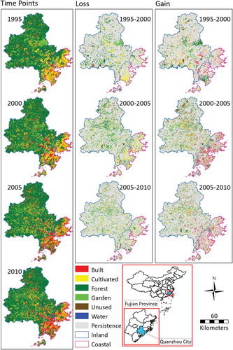
Figure 1 shows Quanzhou stratified into two regions: Inland and Coastal. Inland consists of Luojiang District, Nan’an City, Dehua County, Yongchun County, and Anxi County. Coastal consists of Quangang District, Licheng District, Fengze District, Jinjiang City, Shishi City, Hui’an County, and Jinmen County. A map overlay of each pair of consecutive time points generates a transition matrix for each region. Table 1 gives the six transition matrices that derive from the two regions and three time intervals. The six matrices are the inputs to Intensity Analysis.

Table 1. Transition matrices for two regions during three time intervals in square kilometers where Start indicates the start year of each 5-year time interval t.

		To	To	To	To	To	To
Start	From	Built	Cultivated	Forest	Garden	Unused	Water
Inland r = 1
1995	Built	239	16	14	5	0	1
1995	Cultivated	104	696	134	138	3	2
1995	Forest	79	277	5699	125	164	10
1995	Garden	22	91	168	489	2	1
1995	Unused	5	8	195	4	196	0
1995	Water	2	2	6	1	0	61
2000	Built	222	86	99	30	8	6
2000	Cultivated	107	507	311	115	40	9
2000	Forest	71	353	5384	220	157	30
2000	Garden	38	174	214	309	22	5
2000	Unused	3	23	168	13	158	1
2000	Water	3	8	13	1	1	51
2005	Built	324	55	42	15	3	5
2005	Cultivated	107	638	240	127	27	12
2005	Forest	77	245	5633	126	86	23
2005	Garden	31	91	180	374	9	3
2005	Unused	10	26	65	13	269	2
2005	Water	5	9	16	2	1	70
Coastal r = 2
1995	Built	301	14	4	1	0	2
1995	Cultivated	124	824	120	2	4	5
1995	Forest	13	49	397	18	8	3
1995	Garden	4	12	4	52	0	0
1995	Unused	4	3	6	3	72	2
1995	Water	8	6	2	1	2	34
2000	Built	353	53	39	4	3	2
2000	Cultivated	230	548	94	7	18	11
2000	Forest	56	47	416	4	7	2
2000	Garden	18	8	12	27	11	0
2000	Unused	9	14	19	2	42	3
2000	Water	8	6	4	1	0	25
2005	Built	568	69	24	4	5	3
2005	Cultivated	129	476	46	10	11	6
2005	Forest	67	63	421	15	17	3
2005	Garden	11	4	3	25	0	0
2005	Unused	9	11	5	1	54	0
2005	Water	4	5	2	0	3	29

Figure 1. Maps of Quanzhou City, Fujian, China.

2.2 Intensity Analysis

2.2.1 Interval level

Table 2 presents the mathematical notation to analyze the transition matrices. Subscript r denotes the two regions of Quanzhou thus r = 1, 2. Subscript t denotes the time interval thus t = 1, 2, 3. Subscripts i and j denote the categories. The number of categories is J, which is six for Quanzhou. Each entry C_rtij within a transition matrix is the size in region r that transitions during interval t from category i to category j. If i = j, then both C_rtii and C_rtjj are the size in region r that persists during interval t as the category. For example in Table 1, C₁₁₆₆ = 61, C₁₂₃₄ = 220, C₁₃₅₄ = 13, C₂₁₃₃ = 397, C₂₂₅₃ = 19, and C₂₃₁₁ = 568.

Table 2. Mathematical notation.

Symbol	Meaning
Crtii	Size of region r that persists during interval t as category i
Crtij	Size of region r that transitions during interval t from category i to category j
Crtji	Size of region r that transitions during interval t from category j to category i
Crtjj	Size of region r that persists during interval t as category j
Drt	Change intensity as percentage of region r during interval t
Ert	Exchange component of change intensity as percentage of region r during interval t
Grtj	Gain intensity in region r during interval t for category j relative to size of category j at end of interval t
i	Index for a category where i = 1, 2, …, J
j	Index for a category where j = 1, 2, …, J
J	Number of categories, which is six for Quanzhou
Lrti	Loss intensity in region r during interval t for category i relative to size of category i at start of interval t
Qrt	Quantity component of change intensity as percentage of region r during interval t
r	Index for a region where r = 1, 2 for Quanzhou
Rrtij	Transition intensity in region r during interval t from category i to category j relative to size of category i at start of interval t
Srt	Shift component of change intensity as percentage of region r during interval t
t	Index for a time interval where t = 1, 2, 3 for Quanzhou
Wrtj	Uniform transition intensity in region r during interval t for gain of category j relative to the size of region r that is not j at start of interval t

Intensity Analysis’ interval level compares the time intervals in terms of size and intensity of gross change in each region. Equation 1 defines the size of gross change in region r during interval t. Equations 2–4 separate the gross change in region r during interval t into three components: quantity, exchange, and shift (Pontius Jr 2019). Equation 2 defines the quantity component, which measures the absolute net change in the sizes of the categories. Each change involves two categories: a losing category and a gaining category. Thus, the numerator of equation 2 is double the absolute net change, which is why equation 2 divides by two. The quantity component is less than the gross change when any category experiences simultaneous loss and gain during a time interval. Equation 3 defines the exchange component. Exchange occurs when category i transitions to category j in some places while category j transitions to category i in other places within a region during a time interval. Equation 4 defines the shift component. Shift for category i occurs when both C_rtij < C_rtji and C_rtik > C_rtki for at least one combination of categories j and k. Equation 4 reflects the fact that gross change is the sum of its three components. Equations 5–8 define the intensity of gross change and its components as a percentage of region r during interval t.

(1) $Chang{e}_{rt}={\sum }_{i=1}^J\left[\left({\sum }_{j=1}^J{C}_{rtij}\right)-C_{rtii}\right]$(1)

(2) $Quantit{y}_{rt}=\left[{\sum }_{i=1}^J\left|{\sum }_{j=1}^J\left(C_{rtij}-C_{rtji}\right)\right|\right]/2$(2)

(3) $Exchang{e}_{rt}={\sum }_{i=1}^J\left\{\left[{\sum }_{j=1}^J\mathrm{M}\mathrm{I}\mathrm{N}\mathrm{I}\mathrm{M}\mathrm{U}\mathrm{M}\left(C_{rtij},C_{rtji}\right)\right]-C_{rtii}\right\}$(3)

(4) $Shif{t}_{rt}=Chang{e}_{rt}-Quantit{y}_{rt}-Exchang{e}_{rt}$(4)

(5) $D_{rt}=\frac{Chang{e}_{rt}100\mathrm{\%}}{\mathrm{s}\mathrm{i}\mathrm{z}\mathrm{e}\mathrm{o}\mathrm{f}\mathrm{r}\mathrm{e}\mathrm{g}\mathrm{i}\mathrm{o}\mathrm{n}r}=\frac{Chang{e}_{rt}100\mathrm{\%}}{{\sum }_{i=1}^J\left({\sum }_{j=1}^J{C}_{rtij}\right)}$(5)

(6) $Q_{rt}=\frac{Quantit{y}_{rt}100\mathrm{\%}}{\mathrm{s}\mathrm{i}\mathrm{z}\mathrm{e}\mathrm{o}\mathrm{f}\mathrm{r}\mathrm{e}\mathrm{g}\mathrm{i}\mathrm{o}\mathrm{n}r}=\frac{Quantit{y}_{rt}100\mathrm{\%}}{{\sum }_{i=1}^J\left({\sum }_{j=1}^J{C}_{rtij}\right)}$(6)

(7) $E_{rt}=\frac{Exchang{e}_{rt}100\mathrm{\%}}{\mathrm{s}\mathrm{i}\mathrm{z}\mathrm{e}\mathrm{o}\mathrm{f}\mathrm{r}\mathrm{e}\mathrm{g}\mathrm{i}\mathrm{o}\mathrm{n}r}=\frac{Exchang{e}_{rt}100\mathrm{\%}}{{\sum }_{i=1}^J\left({\sum }_{j=1}^J{C}_{rtij}\right)}$(7)

(8) $S_{rt}=\frac{Shif{t}_{rt}100\mathrm{\%}}{\mathrm{s}\mathrm{i}\mathrm{z}\mathrm{e}\mathrm{o}\mathrm{f}\mathrm{r}\mathrm{e}\mathrm{g}\mathrm{i}\mathrm{o}\mathrm{n}r}=\frac{Shif{t}_{rt}100\mathrm{\%}}{{\sum }_{i=1}^J\left({\sum }_{j=1}^J{C}_{rtij}\right)}$(8)

2.2.2 Category level

Intensity Analysis’ category level compares the categories in terms of size and intensity of loss and gain in each region during each time interval (Pontius Jr et al. 2013). Equation 9 defines L_rti as the loss intensity from category i, which is the percentage of the start size of category i that loses during the time interval. Equation 10 defines G_rtj as the gain intensity to category j, which is the percentage of the end size of category j that gained during the time interval. The intensity of a uniform change in region r during interval t is D_rt. If L_rti<D_rt or G_rtj<D_rt then we say the respective loss from category i or gain to category j in region r during interval t is dormant. If L_rti>D_rt or G_rtj>D_rt then we say the respective loss from category i or gain to category j in region r during interval t is active. If L_rti= D_rt or G_rtj= D_rt then we say the respective loss from category i or gain to category j in region r during interval t is uniform.

(9) $L_{rti}=\frac{\left[\mathrm{l}\mathrm{o}\mathrm{s}\mathrm{s}\mathrm{o}\mathrm{f}i\mathrm{i}\mathrm{n}\mathrm{r}\mathrm{e}\mathrm{g}\mathrm{i}\mathrm{o}\mathrm{n}r\mathrm{d}\mathrm{u}\mathrm{r}\mathrm{i}\mathrm{n}\mathrm{g}\mathrm{i}\mathrm{n}\mathrm{t}\mathrm{e}\mathrm{r}\mathrm{v}\mathrm{a}\mathrm{l}t\right]100\mathrm{\%}}{\mathrm{s}\mathrm{i}\mathrm{z}\mathrm{e}\mathrm{o}\mathrm{f}i\mathrm{i}\mathrm{n}\mathrm{r}\mathrm{e}\mathrm{g}\mathrm{i}\mathrm{o}\mathrm{n}r\mathrm{a}\mathrm{t}\mathrm{s}\mathrm{t}\mathrm{a}\mathrm{r}\mathrm{t}\mathrm{o}\mathrm{f}\mathrm{i}\mathrm{n}\mathrm{t}\mathrm{e}\mathrm{r}\mathrm{v}\mathrm{a}\mathrm{l}t}=\frac{\left[\left({\sum }_{j=1}^J{C}_{rtij}\right)-C_{rtii}\right]100\mathrm{\%}}{{\sum }_{j=1}^J{C}_{rtij}}$(9)

(10) $G_{rtj}=\frac{\left[\mathrm{g}\mathrm{a}\mathrm{i}\mathrm{n}\mathrm{o}\mathrm{f}j\mathrm{i}\mathrm{n}\mathrm{r}\mathrm{e}\mathrm{g}\mathrm{i}\mathrm{o}\mathrm{n}r\mathrm{d}\mathrm{u}\mathrm{r}\mathrm{i}\mathrm{n}\mathrm{g}\mathrm{i}\mathrm{n}\mathrm{t}\mathrm{e}\mathrm{r}\mathrm{v}\mathrm{a}\mathrm{l}t\right]100\mathrm{\%}}{\mathrm{s}\mathrm{i}\mathrm{z}\mathrm{e}\mathrm{o}\mathrm{f}j\mathrm{i}\mathrm{n}\mathrm{r}\mathrm{e}\mathrm{g}\mathrm{i}\mathrm{o}\mathrm{n}r\mathrm{a}\mathrm{t}\mathrm{e}\mathrm{n}\mathrm{d}\mathrm{o}\mathrm{f}\mathrm{i}\mathrm{n}\mathrm{t}\mathrm{e}\mathrm{r}\mathrm{v}\mathrm{a}\mathrm{l}t}=\frac{\left[\left({\sum }_{i=1}^J{C}_{rtij}\right)-C_{rtjj}\right]100\mathrm{\%}}{{\sum }_{i=1}^J{C}_{rtij}}$(10)

2.2.3 Transition level

Intensity Analysis’ transition level compares the transitions in terms of size and intensity in each region during each time interval. Equation 11 defines R_rtij as the transition intensity from category i to category j where i≠ j. Equation 12 defines W_rtj as the uniform transition intensity to category j. If R_rtij<W_rtj then we say the gain of j avoids i in region r during interval t. If R_rtij>W_rtj then we say the gain of j targets i in region r during interval t. If R_rtij= W_rtj then we say the gain of j is uniform with respect to i in region r during interval t (Pontius Jr et al. 2013).

(11) $R_{rtij}=\frac{\left(\mathrm{t}\mathrm{r}\mathrm{a}\mathrm{n}\mathrm{s}\mathrm{i}\mathrm{t}\mathrm{i}\mathrm{o}\mathrm{n}\mathrm{f}\mathrm{r}\mathrm{o}\mathrm{m}i\mathrm{t}\mathrm{o}j\mathrm{i}\mathrm{n}\mathrm{r}\mathrm{e}\mathrm{g}\mathrm{i}\mathrm{o}\mathrm{n}r\mathrm{d}\mathrm{u}\mathrm{r}\mathrm{i}\mathrm{n}\mathrm{g}\mathrm{i}\mathrm{n}\mathrm{t}\mathrm{e}\mathrm{r}\mathrm{v}\mathrm{a}\mathrm{l}t\right)100\mathrm{\%}}{\mathrm{s}\mathrm{i}\mathrm{z}\mathrm{e}\mathrm{o}\mathrm{f}i\mathrm{i}\mathrm{n}\mathrm{r}\mathrm{e}\mathrm{g}\mathrm{i}\mathrm{o}\mathrm{n}r\mathrm{a}\mathrm{t}\mathrm{s}\mathrm{t}\mathrm{a}\mathrm{r}\mathrm{t}\mathrm{o}\mathrm{f}\mathrm{i}\mathrm{n}\mathrm{t}\mathrm{e}\mathrm{r}\mathrm{v}\mathrm{a}\mathrm{l}t}=\frac{\left(C_{rtij}\right)100\mathrm{\%}}{{\sum }_{j=1}^J{C}_{rtij}}$(11)

(12) $W_{rtj}=\frac{\left[\mathrm{g}\mathrm{a}\mathrm{i}\mathrm{n}\mathrm{o}\mathrm{f}j\mathrm{i}\mathrm{n}\mathrm{r}\mathrm{e}\mathrm{g}\mathrm{i}\mathrm{o}\mathrm{n}r\mathrm{d}\mathrm{u}\mathrm{r}\mathrm{i}\mathrm{n}\mathrm{g}\mathrm{i}\mathrm{n}\mathrm{t}\mathrm{e}\mathrm{r}\mathrm{v}\mathrm{a}\mathrm{l}t\right]100\mathrm{\%}}{\mathrm{s}\mathrm{i}\mathrm{z}\mathrm{e}\mathrm{o}\mathrm{f}\mathrm{n}\mathrm{o}\mathrm{t}j\mathrm{i}\mathrm{n}\mathrm{r}\mathrm{e}\mathrm{g}\mathrm{i}\mathrm{o}\mathrm{n}r\mathrm{a}\mathrm{t}\mathrm{s}\mathrm{t}\mathrm{a}\mathrm{r}\mathrm{t}\mathrm{o}\mathrm{f}\mathrm{i}\mathrm{n}\mathrm{t}\mathrm{e}\mathrm{r}\mathrm{v}\mathrm{a}\mathrm{l}t}=\frac{\left[\left({\sum }_{i=1}^J{C}_{rtij}\right)-C_{rtjj}\right]100\mathrm{\%}}{{\sum }_{i=1}^J\left[\left({\sum }_{j=1}^J{C}_{rtij}\right)-C_{rtji}\right]}$(12)

3 Results

3.1 Interval level and components

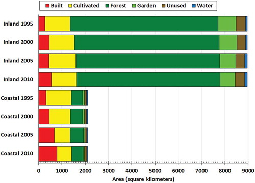
Figure 2 shows the size of each land category at four time points for Quanzhou, where the Inland region is 4.3 times larger than the Coastal region. The Inland region is mostly Forest at all time points. In the Coastal region, the largest category is Cultivated at 1995, 2000, and 2005, then Built at 2010. Figure 2 is important for the interpretation of Intensity Analysis because Figure 2 shows the sizes of the various denominators in equations 5–12. Figure 2 reflects each category’s net changes. During 1995–2010, Forest experiences net loss while Built experiences net gain, both equivalent to 2% of the Inland region. Meanwhile, Cultivated experiences net loss while Built experiences net gain, both equivalent to approximately 22% of the Coastal region.

Figure 2. Area of each land category in Quanzhou’s two regions at four time points.

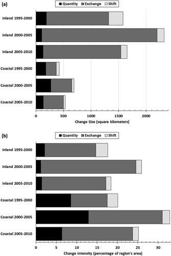
Figure 3a shows that change in the Inland region is larger than change in the Coastal region. Figure 3b shows that change as a percentage of the Inland region is less than change as a percentage of the Coastal region during each respective time interval. Thus, change is larger in the Inland region because the Inland region occupies a larger spatial extent and in spite of the fact that change is more intensive in the Coastal region. Figure 3 shows also that change in both regions is fastest during the middle time interval. Figure 3 shows the gross change during each interval separated into its three components: quantity, exchange, and shift. The quantity component accounts for less than half of the change in both regions during all intervals. This implies that most of the change is loss of a category accompanied by gain of the same category within a region. Exchange is the largest component in both regions during all intervals, as transitions from i to j occur simultaneously with transitions from j to i.

Figure 3. Interval level change components in terms of (a) size and (b) intensity.

3.2 Category level

Figure 4a shows the size of the loss and gain of each category in terms of area, thus indicates whether each category’s net change is negative, zero or positive. One must focus on the categories that have the largest losses and gains to develop insight concerning most of the change. In the Inland region, Forest and Cultivated have the largest losses and gains during all intervals. In the Coastal region, Cultivated has the largest loss while Built has the largest gain during each interval. There are two reasons why a category could experience a large loss. First, a uniform change intensity would cause categories that are larger at the start time to experience larger losses. Second, a category’s loss could be more intensive than uniform. One must consider a category’s loss intensity relative to the uniform change intensity to see whether each of the reasons apply.

Figure 4. Category level losses and gains in terms of (a) size and (b) intensity.

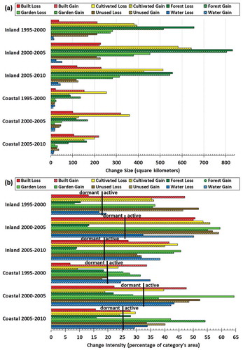
Figure 4b shows the uniform change intensity as a black line for each region during each time interval, which is equivalent to each respective intensity in Figure 3b. The bars in Figure 4b show each category’s intensity of loss and gain in terms of change per area of the category. If a bar stops before the uniform line, then the change is dormant. If a bar extends beyond the uniform line, then the change is active. In the Inland region, Forest is the only category that is dormant for both loss and gain during all time intervals. Forest’s large size in the denominator of its intensity causes Forest’s intensity to be dormant. Therefore, Forest’s large size is the single reason for its large losses in the Inland region. For both regions during all intervals, Cultivated loses actively, meaning more intensively than uniform. Thus, two reasons explain Cultivated’s large losses. The first reason is Cultivated’s relatively large size and the second reason is Cultivated’s intensively active loss. The proportion of the bar that extends beyond the uniform line is the proportion of the loss that the second reason explains. In the Inland region, more than half of the bar for Cultivated’s loss extends beyond the uniform line during each time interval, which indicates that active intensity is more important than start size to explain the size of Cultivated’s loss. In the Coastal region, less than half of each bar for Cultivated’s loss extends beyond the uniform line during each time interval, which indicates that active intensity is less important than start size to explain the size of Cultivated’s loss. The gain intensity for a category is the percentage of a category’s end size that derives from gain during the time interval. Built, Garden, and Water are the categories that have active gains in both regions during all intervals.

Gains to Built, Cultivated, and Forest account for between 70% and 90% of the change in each region during each time interval. Therefore, the transition level analyzes transitions to those three categories.

3.3 Transition level

Figure 5 shows results for transition level analysis. For transitions to Built, Figure 5a shows sizes while Figure 5b shows intensities, similar in logic to parts a and b in Figures 3–4. Built gains most from Cultivated in both regions during all intervals because of two reasons. First, Cultivated is larger than most categories; thus, a uniform gain of Built would cause the transition from Cultivated to be larger than from most categories. Second, the gain of Built targets Cultivated, meaning the transition intensity is greater than the uniform transition intensity. In the Inland region, more than half of the bar for Cultivated extends beyond the uniform line, which indicates that Culitvated’s transition intensity is more important than Cultivated’s start size to explain the size of the transition. In the Coastal region, less than half of each transition intensity bar for Cultivated extends beyond the uniform line, which indicates that Cultivated’s transition intensity is less important than Cultivated’s start size to explain the size of the transition. Built gains second-most from Forest, while Figure 5b shows that the gain of Built avoids Forest in both regions during all intervals. Therefore, Forest’s relatively large start size is the only reason for the large transitions from Forest to Built.

Figure 5. Transitions to built in (a) size and (b) intensity, transitions to cultivated in (c) size and (d) intensity, and transitions to forest in (e) size and (f) intensity.

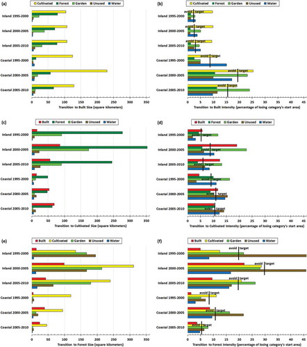
Figure 5c-d shows transitions to Cultivated. Most of the largest transitions are from Forest in terms of size. Transition intensities reveal that gain of Cultivated avoids Forest in most cases. Thus, Forest’s relatively large size is the main reason that Cultivated gains more from Forest than from the other categories.

Figure 5e-f shows transitions to Forest. Most of the largest transitions are from Cultivated in terms of size. Cultivated is the largest non-Forest category at the start of each time interval in both regions. Transition intensities reveal that the gain of Forest avoids Cultivated during three of the six intervals. Thus, Cultivated’s large start size explains the large transitions from Cultivated to Forest during those three intervals. Forest gains the most from Unused in the Inland region during 1995–2000, in spite of Unused’s small size at 1995. Forest’s targeting intensity explains most of the transition from Unused to Forest in the Inland region during 1995–2000.

Comparison across the clusters of bars in Figure 5 reveals how a particular losing category transitions to other categories in each region during each time interval. For example, Unused loses more to Forest than to Built or Cultivated in the Inland region during 1995–2000 because of two reasons. First, the variation among the uniform transition intensity lines shows that Forest gains more aggressively than Built or Cultivated in the Inland region. So, even if the transition intensity bars were equal to their respective uniform line, then the categories would lose more to Forest than to Built or Cultivated in the Inland region. Second, Forest’s gain targets Unused while the gains of both Built and Cultivated avoid Unused in the Inland region during 1995–2000.

4 Discussion

4.1 Data quality

Intensity Analysis is helpful because it reveals clearly the sizes and intensities of the transitions, which helps readers to consider the possible reasons for the apparent transitions. For example, Figure 5c shows large transitions from Built to Cultivated, while Figure 5d shows that Cultivated’s gain sometimes targets Built. China’s land consolidation project has converted some land from Built to Cultivated (Yu et al. 2018). However, we suspect data error might account for some of the apparent transition from Built to Cultivated. We have seen this same transition in other datasets, specifically in GlobeLand30 (Shafizadeh-Moghadam et al. 2019). Perhaps it is difficult for classifiers of remotely sensed images to differentiate between Built and Cultivated, especially when the two categories exist in close proximity to each other, as they frequently do in Asia. Counter-intuitive transitions should guide the research agenda because the most important next step might be to consider data errors in more depth than overall percent correct conveys. In some cases, a large exchange component signals data errors (Pontius Jr 2019). The transition from Built to Cultivated paired with the transition from Cultivated to Built contributes to the exchange component in Figure 3, which warrants investigation concerning possible data error in Quanzhou. Data errors are likely to influence the analysis’ details, thus researchers should focus on the largest and more intensive signals of change, which Intensity Analysis distinguishes from the smaller and less intensive signals of change. A next step is to quantify the errors that could account for the deviations between observed intensities and uniform intensities by using the methods of (Aldwaik and Pontius Jr 2013).

4.2 Pattern and process

Scientists frequently want to link land change patterns with processes (De Alban et al. 2019; Pontius Jr 2006; Václavík and Rogan 2009; Cunningham et al. 2015). Intensity Analysis is a helpful step to account for land change patterns before scientists try to use additional variables to link patterns with processes. If scientists do not understand the patterns, then scientists might search for processes that do not exist. For example, Figure 5a shows that the largest transitions to Built derive from Cultivated and Forest. However, Cultivated differs from Forest concerning the reasons for their transitions to Built. Figure 5b shows that Built’s gain targets Cultivated and avoids Forest. Thus, the transition from Forest to Built is large because of Forest’s large start size and in spite of the fact that Built’s gain avoids Forest. The transition from Cultivated to Built is large for two reasons. First, Cultivated’s start size is larger than most categories. Second, Built’s gain targets Cultivated. Consequently, a resulting question is “What processes drive builders to target Cultivated and to avoid Forest?” Figure 5b shows also that more than half of Cultivated’s intensity bar is to the right of the uniform line in the Inland region, which means that Built’s targeting of Cultivated explains most of the transition from Cultivated to Built in the Inland region. Meanwhile, more than half of Cultivated’s intensity bar is to the left of the uniform line in the Coastal region, which means that Cultivated’s size explains most of the transition from Cultivated to Built in the Coastal region. Thus, another question for future research is “For the transition from Cultivated to Built, why does the targeting intensity explain more than half of the transition in the Inland region and less than half of the transition in the Coastal region?”

Intensity Analysis addresses a particular question concerning the comparison of transitions across a matrix’s row, which gives a category’s losses. The question is “Is one transition larger than another transition within a losing category’s row because one category gains more aggressively than another category gains in general, or because one gaining category targets the specific losing category more intensively than another gaining category targets the specific losing category?” A careful reading of Figure 5 answers this question. The black lines in Figure 5 show the uniform transition intensity for each region for each time interval for three gaining categories: Built, Cultivated, and Forest. A gaining category’s uniform transition intensity indicates how aggressively the category gains across the extent that was not the gaining category at the start time. One must compare the uniform transition intensities among gaining categories within a particular region and time interval. For example, consider Garden’s loss from the Inland region during 2000–2005 in Figure 5. Garden loses to Built the least and to Forest the most in terms of size. The three uniform intensity lines for transitions to Built, Cultivated, and Forest show that Built gains the least aggressively and Forest gains the most aggressively in general. Thus, the size of the transition from Garden to Built is smallest because Built gains the least aggressively in general as Built’s uniform transition line indicates, and in spite of the fact that Built’s gain targets Garden. The size of the transition from Garden to Forest is largest because Forest gains the most aggressively in general as Forest’s uniform transition line indicates, and in spite of the fact that Forest’s gain avoids Garden. Our previous publications concerning Intensity Analysis did not give this insight concerning interpretation. Our previous literature might have led readers to misinterpret the gain intensity of equation 10. All categories are equally aggressive in their gains when their uniform transition intensity lines are identical, not necessarily when the gain intensities at the category level are identical. The gain intensity is not appropriate to address the question at the beginning of this paragraph.

Equation 10 defines a category’s gain intensity where the denominator is the category’s size at the end of the time interval, which assures that it makes sense to compare the gain intensity to the time interval’s uniform change intensity in equation 5. A category’s gain intensity is the percentage of its end size that derives from its gain during the time interval. A category’s end size is its start size plus its gain size minus its loss size. Readers must not interpret the gain intensity in equation 10 as the percent gain from interval’s start time. Some other literature expresses a category’s change as a ratio with net change in the numerator and the category’s start size in the denominator (Liu et al. 2018; Quan et al. 2015), which is not the same as the gain intensity of Intensity Analysis. If the denominator of equation 10 were the category’s start size, then two potential problems would occur. First, the result could be greater than 100%, thus comparison to the interval’s uniform intensity would not make sense. Second, if the category’s start size were zero, then the gain intensity would be undefined, even when the category exists at the end time.

If the goal is to compare the sizes of transitions that share neither a row nor a column within a matrix, then Intensity Analysis shows how it is helpful to account for three factors. The first factor is the losing category’s start size, which is the sum across the losing category’s row. The second factor is the gaining category’s uniform transition intensity, which indicates the aggressiveness of the gain within the gaining category’s column. The third factor is the deviation between the uniform transition intensity and the specific transition intensity, which determines whether the gain within the column category avoids or targets the row category.

4.3 Relationship to previous literature

Our article’s equations are different from the original version of Intensity Analysis in two respects. First, this article’s equations have notation for three components and multiple regions, whereas the original version of Intensity Analysis did not. Second, this article’s equations exclude the mathematics to convert change into annual rates, because each time interval is the same duration in this article. Our modifications do not influence Intensity Analysis with respect to the interpretation of dormant, active, avoid, and target. The insights that this Discussion section gives concerning interpretation apply also to the original version of Intensity Analysis.

The original version of Intensity Analysis had two additional equations to analyze intensities of transitions from a losing category as percentages of the sizes of the categories at the end of the time interval, specifically equations 7–8 in Aldwaik and Pontius Jr (2012). We now realize that those transition intensities do not have a straightforward interpretation when analyzing temporal change, because transitions during the time interval influence the categories’ end sizes (Pontius Jr et al. 2013). Therefore, we use the transition intensities in our equations 11–12 and not the concepts of equations 7–8 in Aldwaik and Pontius Jr (2012). Furthermore, we do not include equations 7–8 from Aldwaik and Pontius Jr (2012) in the Intensity Analysis package in the language R (Khallaghi and Pontius Jr 2019). Consequently, we do not use the definition of “systematic” in previous literature (Alo and Pontius Jr 2008). However, those two transition intensities that we exclude are relevant when the sum in each column is independent of the entries in the table, such as in a confusion matrix that shows classification errors where the columns are the ground information, which exists independently of the classification (Christman et al. 2015). For such a confusion matrix, the sum of each row depends on the entries in the table; therefore, equations 11–12 in our paper would not be relevant. Further explanation exists in Pontius Jr (2020).

The original version of Intensity Analysis divides the metrics by the duration of the time interval because the original method analyzes time intervals that have various durations. Our equations do not divide by the duration because each time interval has the same duration. Therefore, readers avoid the possible confusion concerning the meaning of annual change rate, because there are various ways to express an annual change rate. If we were to have divided by the duration, then equation 5 would express annual change percentage in a manner identical to the original intention of the comprehensive land use dynamic degree (CLUDD). CLUDD is popular particularly in China (B. Huang et al. 2018). The mathematical notation in much of the literature that uses CLUDD is confusing to the point that authors have computed CLUDD in various ways that do not reflect the original intention of CLUDD. For example, two recent articles in the same journal report CLUDD as equations that are not equivalent to each other (Wei et al. 2018; Zhang et al. 2015). This inspired recommendations for rules to write mathematics clearly (Pontius Jr et al. 2017a). Our article uses the recommendations to express equations in both words and mathematical notation.

If literature reports clearly the computation of annual change percentage, then readers can compare across various case studies (Akinyemi, Pontius Jr, and Braimoh 2017; F. Huang et al. 2018; Huang et al. 2012; Teixeira, Marques, and Pontius Jr 2016; Villamor, Pontius Jr, and van Noordwijk 2014; Zhou et al. 2014; Estoque and Murayama 2015; Shafizadeh-Moghadam et al. 2019). Scientists must consider scales of space, time, and category when comparing cases (Aldwaik, Onsted, and Pontius Jr 2015). It is clearer to compare cases when the scales of the cases are more similar. For example, Intensity Analysis served as the framework to compare three time intervals of land change outside versus inside the coastal zone of Longhai, China (B. Huang et al. 2018). That research shows patterns in Longhai similar to patterns in Quanzhou, where change is more intensive closer to the coast while change is fastest during the middle time interval. This temporal non-stationarity is inconsistent with the assumptions of simulation models that extrapolate business-as-usual scenarios (Pontius Jr et al. 2018). Intensity Analysis is helpful to test whether the historic data indicate that business has been usual, i.e., has been stationary.

4.4 Implications for extrapolation

It is important to distinguish between a transition’s size versus its intensity when using a model that simulates the future gain of a particular category. The Land Change Modeler in the software TerrSet endorses evidence likelihoods, which TerrSet sometimes calls empirical likelihoods. In contrast, the Geomod model uses a different concept called empirical probabilities (Eastman 2014; Eastman, Van Fossen, and Solorzanó 2005; Pontius Jr, Cornell, and Hall 2001). If the map of land categories serves as an independent variable to explain a particular category’s gain, then a transition’s evidence likelihood is a proportion computed as the size of the transition divided by the size of the particular category’s gain. In contrast, a transition’s empirical probability is a proportion computed as the size of the transition divided by the size of the losing category at the start time, which is identical to our article’s transition intensity in equation 11. Figure 5 illustrates how evidence likelihoods differ from empirical probabilities for the Inland region. Figure 5c shows that Cultivated gains most from Forest, thus Cultivated’s evidence likelihood is greatest from Forest. Figure 5d shows that Cultivated gains most intensively from Garden, thus Cultivated’s empirical probability is greatest from Garden. Cultivated’s transition size is largest from Forest, simply because Forest is the largest category at the start time. Intensity Analysis reveals that Culitvated’s gain avoids Forest and targets Garden. If a simulation were to use evidence likelihood to create a transition potential map, then the simulation would allocate Cultivated’s future gain from Forest, in spite of the fact that Cultivated’s gain avoids Forest according to the historic pattern. If a simulation were to use empirical probabilities to create a transition potential map, then the simulation would allocate Cultivated’s future gain from Garden in a manner that extrapolates the historic pattern concerning how Cultivated’s gain targets Garden. The debate between evidence likelihood and empirical probabilities applies also to when scientists explain the gain of a category with respect to other independent variables, such as topographic slope, political units, proximity to roads, etc. (Chen and Pontius Jr 2010).

5 Conclusion

This article presents developments in methodology and insights concerning interpretation for Intensity Analysis. This article’s equations are more elaborate than the original version of Intensity Analysis with respect to difference components and regions but are simpler with respect to time because each time interval has the same duration in this article. This article’s insights concerning interpretation apply also to the original version of Intensity Analysis. The first new insight expresses the proportion of a change that is attributable to the losing category’s start size versus the deviation from a uniform intensity. The second insight warns of possible misinterpretation of gain intensity and instead shows how each category’s uniform transition intensity indicates the aggressiveness of each category’s gain.

The methodology compares Quanzhou’s Inland region to its Coastal region at three levels: interval, category, and transition. The interval level shows that Coastal change is more intensive than Inland change as a percentage of each region. In both regions, the overall change is not stationary through time, as change is fastest during the middle of the three time intervals. Exchange is the largest component of change in both regions during all intervals, which might signal data error. The category level shows that during all time intervals, the Inland region has net loss of Forest and Garden, while the Coastal region has net loss of Cultivated and net gain of Built. Actively intense changes include losses from Cultivated & Garden and gains to Built in both regions during all intervals. The transition level indicates that Built’s gain targets Cultivated and avoids Forest in both regions during all intervals. Built’s targeting of Cultivated accounts for most of the transition from Cultivated to Built in the Inland region, while Cultivated’s size accounts for most of the transition from Cultivated to Built in the Coastal region. Much of Cultivated’s gain derives from Forest, which is attributable to Forest’s large size. The largest transitions to Forest tend to derive from Cultivated, as Cultivated’s size is the largest among the non-Forest categories in both regions at the start of all time intervals. It is not yet clear how errors in the data could influence these results. Nevertheless, these results are consistent with other reports from China, where policymakers are concerned with loss of agricultural land.

Readers can apply Intensity Analysis to their own data by using packages in the language R to compute components and intensities (Khallaghi and Pontius Jr 2019; Pontius Jr and Santacruz 2015). Readers can also use the spreadsheets called PontiusMatrix.xlsx and IntensityAnalysis03.xlsm, which are available for free at www.clarku.edu/~rpontius.

Acknowledgements

Key Project of Hunan Provincial Education Department of China and Recruitment Program of High-end Foreign Experts of the State Administration of Foreign Experts Affairs of China funded this work via grant 17A067 and grant GWD201543000243. The China Scholarship Council Recruitment funded this work via grant 201808430277. The Talent Introduction Project of Hengyang Normal University also supported this work via grant 17D03. The United States National Science Foundation’s Division of Environmental Biology supported this work via grant OCE-1637630 for the Plum Island Ecosystems Long Term Ecological Research site. Opinions, findings, conclusions, and recommendations in this article are those of the authors and do not necessarily reflect those of the funders.

Disclosure statement

No potential conflict of interest was reported by the authors.

Additional information

Funding

This work was supported by the China Scholarship Council [201808430277]; Education Department of Hunan Province [17A067]; Hengyang Normal University [17D03]; United States National Science Foundation [OCE-1637630]; State Administration of Foreign Experts Affairs [GWD201543000243].

References

- Akinyemi, F. O., R. G. Pontius Jr, and A. K. Braimoh. 2017. “Land Change Dynamics: Insights from Intensity Analysis Applied to an African Emerging City.” Journal of Spatial Science 62 (1): 69–83. doi:10.1080/14498596.2016.1196624.
- Aldwaik, S. Z., J. A. Onsted, and R. G. Pontius Jr. 2015. “Behavior-Based Aggregation of Land Categories for Temporal Change Analysis.” International Journal of Applied Earth Observation and Geoinformation 35 (Mar): 229–238. doi:10.1016/j.jag.2014.09.007.
- Aldwaik, S. Z., and R. G. Pontius Jr. 2012. “Intensity Analysis to Unify Measurements of Size and Stationarity of Land Changes by Interval, Category, and Transition.” Landscape and Urban Planning 106 (1): 103–114. doi:10.1016/j.landurbplan.2012.02.010.
- Aldwaik, S. Z., and R. G. Pontius Jr. 2013. “Map Errors that Could Account for Deviations from a Uniform Intensity of Land Change.” International Journal of Geographical Information Science 27 (9): 1717–1739. doi:10.1080/13658816.2013.787618.
- Alo, C. A., and R. G. Pontius Jr. 2008. “Identifying Systematic Land-Cover Transitions Using Remote Sensing and GIS: The Fate of Forests Inside and Outside Protected Areas of Southwestern Ghana.” Environment and Planning B: Planning and Design 35 (2): 280–295. doi:10.1068/b32091.
- Awotwi, A., G. K. Anornu, J. A. Quaye-Ballard, and T. Annor. 2018. “Monitoring Land Use and Land Cover Changes Due to Extensive Gold Mining, Urban Expansion, and Agriculture in the Pra River Basin of Ghana, 1986-2025.” Land Degradation & Development 29 (10): 3331–3343. doi:10.1002/ldr.3093.
- Berlanga-Robles, C. A., and A. Ruiz-Luna. 2011. “Integrating Remote Sensing Techniques, Geographical Information Systems (GIS), and Stochastic Models for Monitoring Land Use and Land Cover (LULC) Changes in the Northern Coastal Region of Nayarit, Mexico.” GIScience & Remote Sensing 48 (2): 245–263. doi:10.2747/1548-1603.48.2.245.
- Chen, H., and R. G. Pontius Jr. 2010. “Diagnostic Tools to Evaluate a Spatial Land Change Projection along a Gradient of an Explanatory Variable.” Landscape Ecology 25 (9): 1319–1331. doi:10.1007/s10980-010-9519-5.
- Christman, Z., J. Rogan, R. Eastman, and B. L. Turner II. 2015. “Quantifying Uncertainty and Confusion in Land Change Analyses: A Case Study from Central Mexico Using MODIS Data.” GIScience & Remote Sensing July: 1–28. doi:10.1080/15481603.2015.1067859.
- Cunningham, S., J. Rogan, D. Martin, V. DeLauer, S. McCauley, and A. Shatz. 2015. “Mapping Land Development through Periods of Economic Bubble and Bust in Massachusetts Using Landsat Time Series Data.” GIScience & Remote Sensing 52 (4): 397–415. doi:10.1080/15481603.2015.1045277.
- De Alban, J., G. Prescott, K. Woods, J. Jamaludin, K. Latt, C. Lim, A. Maung, and E. Webb. 2019. “Integrating Analytical Frameworks to Investigate Land-Cover Regime Shifts in Dynamic Landscapes.” Sustainability 11 (4): 1139. doi:10.3390/su11041139.
- Eastman, J. R., M. E. Van Fossen, and L. A. Solorzanó. 2005. “GIS, Spatial Analysis and Modeling.” In Chapter 17 Transition Potential Modeling for Land Cover Change, edited by D. Maguire, M. Batty, and M. Goodchild, 339–368. Redlands CA: ESRI Press.
- Eastman, J. R. 2014. TerrSet Geospatial Monitoring and Modeling System. Worcester, MA: Clark University.
- Estoque, R. C., and Y. Murayama. 2014. “A Geospatial Approach for Detecting and Characterizing Non-Stationarity of Land-Change Patterns and Its Potential Effect on Modeling Accuracy.” GIScience & Remote Sensing 51 (3): 239–252. doi:10.1080/15481603.2014.908582.
- Estoque, R. C., and Y. Murayama. 2015. “Intensity and Spatial Pattern of Urban Land Changes in the Megacities of Southeast Asia.” Land Use Policy 48 (Nov): 213–222. doi:10.1016/j.landusepol.2015.05.017.
- Feng, Y., and X. Tong. 2018. “Dynamic Land Use Change Simulation Using Cellular Automata with Spatially Nonstationary Transition Rules.” GIScience & Remote Sensing 55 (5): 678–698. doi:10.1080/15481603.2018.1426262.
- Huang, B., J. Huang, R. G. Pontius Jr, and T. Zhenshun. 2018. “Comparison of Intensity Analysis and the Land Use Dynamic Degrees to Measure Land Changes outside versus inside the Coastal Zone of Longhai, China.” Ecological Indicators 89: 336–347. doi:10.1016/j.ecolind.2017.12.057.
- Huang, F., B. Huang, J. Huang, and L. Shenghui. 2018. “Measuring Land Change in Coastal Zone around a Rapidly Urbanized Bay.” International Journal of Environmental Research and Public Health 15 (6): 1059. doi:10.3390/ijerph15061059.
- Huang, J., R. G. Pontius Jr, L. Qingsheng, and Y. Zhang. 2012. “Use of Intensity Analysis to Link Patterns with Processes of Land Change from 1986 to 2007 in a Coastal Watershed of Southeast China.” Applied Geography 34 (May): 371–384. doi:10.1016/j.apgeog.2012.01.001.
- Jokar Arsanjani, J. 2018. “Characterizing and Monitoring Global Landscapes Using GlobeLand30 Datasets: The First Decade of the Twenty-First Century.” International Journal of Digital Earth May: 1–19. doi:10.1080/17538947.2018.1470689.
- Khallaghi, S., and R. G. Pontius Jr. 2019. Intensity.Analysis. https://cran.r-project.org/web/packages/intensity.analysis/
- Liu, L., X. Xinliang, J. Liu, X. Chen, and J. Ning. 2015. “Impact of Farmland Changes on Production Potential in China during 1990–2010.” Journal of Geographical Sciences 25 (1): 19–34. doi:10.1007/s11442-015-1150-6.
- Liu, P., S. Jia, R. Han, and H. Zhang. 2018. “Landscape Pattern and Ecological Security Assessment and Prediction Using Remote Sensing Approach.” Journal of Sensors 2018 (June): 1–14. doi:10.1155/2018/1058513.
- Liu, Z., Z. Yao, H. Huang, S. Wu, and G. Liu. 2014. “Land Use and Climate Changes and Their Impacts on Runoff in the Yarlung Zangbo River Basin, China.” Land Degradation & Development 25 (3): 203–215. doi:10.1002/ldr.1159.
- Minaei, M., H. Shafizadeh-Moghadam, and A. Tayyebi. 2018. “Spatiotemporal Nexus between the Pattern of Land Degradation and Land Cover Dynamics in Iran.” Land Degradation & Development 29 (9): 2854–2863. doi:10.1002/ldr.3007.
- Olsen, L. M., R. A. Washington-Allen, and V. H. Dale. 2005. “Time-Series Analysis of Land Cover Using Landscape Metrics.” GIScience & Remote Sensing 42 (3): 200–223. doi:10.2747/1548-1603.42.3.200.
- Omrani, H., A. Tayyebi, and B. Pijanowski. 2017. “Integrating the Multi-Label Land-Use Concept and Cellular Automata with the Artificial Neural Network-Based Land Transformation Model: an Integrated ML-CA-LTM Modeling Framework.” GIScience & Remote Sensing 54 (3): 283–304. doi:10.1080/15481603.2016.1265706.
- Ouedraogo, I., J. Barron, S. D. Tumbo, and F. C. Kahimba. 2016. “Land Cover Transition in Northern Tanzania: Land Cover Transition in Northern Tanzania.” Land Degradation & Development 27 (3): 682–692. doi:10.1002/ldr.2461.
- Pontius Jr, R. G. 2006. “Pattern to Process.” In Our Earth’s Changing Land: An Encyclopedia of Land-Use and Land-Cover Change, edited by H. Geist Vol. 2, 462. Westport, CT: Greenwood Press.
- Pontius Jr, R. G., Castella, T. de Nijs, Z. Duan, E. Fotsing, N. Goldstein, K. Kok, et al. 2018. “Lessons and Challenges in Land Change Modeling Derived from Synthesis of Cross-Case Comparisons.” In Trends in Spatial Analysis and Modelling, edited by M. Behnisch and G. Meinel. Vol. 19, 143–164, Geotechnologies and the Environment. Cham: Springer International Publishing. doi: 10.1007/978-3-319-52522-8_8.
- Pontius Jr, R. G. 2019. “Component Intensities to Relate Difference by Category with Difference Overall.” International Journal of Applied Earth Observation and Geoinformation 77 (May): 94–99. doi:10.1016/j.jag.2018.07.024.
- Pontius Jr, R. G. 2020. Metrics that Make a Difference. Cham: Springer Nature Switzerland AG.
- Pontius Jr, R. G., and A. Santacruz. 2014. “Quantity, Exchange, and Shift Components of Difference in a Square Contingency Table.” International Journal of Remote Sensing 35 (21): 7543–7554. doi:10.1080/2150704X.2014.969814.
- Pontius Jr, R. G., and A. Santacruz. 2015. DiffeR: Metrics of Difference for Comparing Pairs of Maps (version 0.0-4). https://cran.r-project.org/web/packages/diffeR
- Pontius Jr, R. G., E. Shusas, and M. Menzie. 2004. “Detecting Important Categorical Land Changes while Accounting for Persistence.” Agriculture, Ecosystems & Environment 101 (2–3): 251–268. doi:10.1016/j.agee.2003.09.008.
- Pontius Jr, R. G., J. Huang, W. Jiang, S. Khallaghi, Y. Lin, J. Liu, B. Quan, and Y. Su. 2017a. “Rules to Write Mathematics to Clarify Metrics Such as the Land Use Dynamic Degrees.” Landscape Ecology 32 (12): 2249–2260. doi:10.1007/s10980-017-0584-x.
- Pontius Jr, R. G., J. D. Cornell, and C. A. S. Hall. 2001. “Modeling the Spatial Pattern of Land-Use Change with GEOMOD2: Application and Validation for Costa Rica.” Agriculture, Ecosystems & Environment 85 (1–3): 191–203. doi:10.1016/S0167-8809(01)00183-9.
- Pontius Jr, R. G., R. Krithivasan, L. Sauls, Y. Yan, and Y. Zhang. 2017b. “Methods to Summarize Change among Land Categories across Time Intervals.” Journal of Land Use Science 12 (4): 218–230. doi:10.1080/1747423X.2017.1338768
- Pontius Jr, R. G., Y. Gao, N. Giner, T. Kohyama, M. Osaki, and K. Hirose. 2013. “Design and Interpretation of Intensity Analysis Illustrated by Land Change in Central Kalimantan, Indonesia.” Land 2 (3): 351–369. doi:10.3390/land2030351.
- Quan, B., H. Ren, R. G. Pontius Jr, and P. Liu. 2018. “Quantifying Spatiotemporal Patterns Concerning Land Change in Changsha, China.” Landscape and Ecological Engineering 14 (2): 257–267. doi:10.1007/s11355-018-0349-y.
- Quan, B., Y. Bai, M.J.M. Römkens, K.-T. Chang, H. Song, T. Guo, and S. Lei. 2015. “Urban Land Expansion in Quanzhou City, China, 1995–2010.” Habitat International 48 (Aug): 131–139. doi:10.1016/j.habitatint.2015.03.021.
- Rafiqul, I. M., M. Giashuddin Miah, and Y. Inoue. 2016. “Analysis of Land Use and Land Cover Changes in the Coastal Area of Bangladesh Using Landsat Imagery.” Land Degradation & Development 27 (4): 899–909. doi:10.1002/ldr.2339.
- Shafizadeh-Moghadam, H., A. Asghari, M. Taleai, M. Helbich, and A. Tayyebi. 2017. “Sensitivity Analysis and Accuracy Assessment of the Land Transformation Model Using Cellular Automata.” GIScience & Remote Sensing 54 (5): 639–656. doi:10.1080/15481603.2017.1309125.
- Shafizadeh-Moghadam, H., M. Minaei, Y. Feng, and R. G. Pontius Jr. 2019. “GlobeLand30 Maps Show Four Times Larger Gross than Net Land Change from 2000 to 2010 in Asia.” International Journal of Applied Earth Observation and Geoinformation 78: 240–248. doi:10.1016/j.jag.2019.01.003.
- Shoyama, K., and A. K. Braimoh. 2011. “Analyzing about Sixty Years of Land-Cover Change and Associated Landscape Fragmentation in Shiretoko Peninsula, Northern Japan.” Landscape and Urban Planning 101 (1): 22–29. doi:10.1016/j.landurbplan.2010.12.016.
- Teixeira, Z., J. C. Marques, and R. G. Pontius Jr. 2016. “Evidence for Deviations from Uniform Changes in a Portuguese Watershed Illustrated by CORINE Maps: an Intensity Analysis Approach.” Ecological Indicators 66 (July): 382–390. doi:10.1016/j.ecolind.2016.01.018.
- Václavík, T., and J. Rogan. 2009. “Identifying Trends in Land Use/Land Cover Changes in the Context of Post-Socialist Transformation in Central Europe: A Case Study of the Greater Olomouc Region, Czech Republic.” GIScience & Remote Sensing 46 (1): 54–76. doi:10.2747/1548-1603.46.1.54.
- Varga, O. G., R. G. Pontius Jr, S. K. Singh, and S. Szabó. 2019. “Intensity Analysis and the Figure of Merit’s Components for Assessment of a Cellular Automata – Markov Simulation Model.” Ecological Indicators 101 (June): 933–942. doi:10.1016/j.ecolind.2019.01.057.
- Villamor, G. B., R. G. Pontius Jr, and M. van Noordwijk. 2014. “Agroforest’s Growing Role in Reducing Carbon Losses from Jambi (sumatra), Indonesia.” Regional Environmental Change 14 (2): 825–834. doi:10.1007/s10113-013-0525-4.
- Wang, J., Y. Lin, T. Zhai, H. Ting, Q. Yuan, Z. Jin, and Y. Cai. 2018. “The Role of Human Activity in Decreasing Ecologically Sound Land Use in China.” Land Degradation & Development 29 (3): 446–460. doi:10.1002/ldr.2874.
- Wei, B., Y. Xie, X. Jia, X. Wang, H. Hongjie, and X. Xue. 2018. “Land Use/Land Cover Change and It’s Impacts on Diurnal Temperature Range over the Agricultural Pastoral Ecotone of Northern China.” Land Degradation & Development 29 (9): 3009–3020. doi:10.1002/ldr.3052.
- Xu, H., X. Wang, and G. Xiao. 2000. “A Remote Sensing and GIS Integrated Study on Urbanization with Its Impact on Arable Lands: Fuqing City, Fujian Province, China.” Land Degradation & Development 11 (4): 301–314. doi:10.1002/1099-145X(200007/08)11:4<301::AID-LDR392>3.0.CO;2-N.
- Yang, Y., Y. Liu, X. Di, and S. Zhang. 2017. “Use of Intensity Analysis to Measure Land Use Changes from 1932 to 2005 in Zhenlai County, Northeast China.” Chinese Geographical Science 27 (3): 441–455. doi:10.1007/s11769-017-0876-8.
- Yu, Q., H. Qiong, J. van Vliet, P. H. Verburg, and W. Wenbin. 2018. “GlobeLand30 Shows Little Cropland Area Loss but Greater Fragmentation in China.” International Journal of Applied Earth Observation and Geoinformation 66 (Apr): 37–45. doi:10.1016/j.jag.2017.11.002.
- Zhang, F., T. Tiyip, Z. D. Feng, H.-T. Kung, V. C. Johnson, J. L. Ding, N. Tashpolat, M. Sawut, and D. W. Gui. 2015. “Spatio-Temporal Patterns of Land Use/Cover Changes over the past 20 Years in the Middle Reaches of the Tarim River, Xinjiang, China.” Land Degradation & Development 26 (3): 284–299. doi:10.1002/ldr.2206.
- Zhou, P., J. Huang, R. G. Pontius Jr, and H. Hong. 2014. “Land Classification and Change Intensity Analysis in a Coastal Watershed of Southeast China.” Sensors 14 (7): 11640–11658. doi:10.3390/s140711640.