Mapping Rice Paddies in Complex Landscapes with Convolutional Neural Networks and Phenological Metrics

ABSTRACT

Rice mapping with remote sensing imagery provides an alternative means for estimating crop-yield and performing land management due to the large geographical coverage and low cost of remotely sensed data. Rice mapping in Southern China, however, is very difficult as rice paddies are patchy and fragmented, reflecting the undulating and varied topography. In addition, abandoned lands widely exist in Southern China due to rapid urbanization. Abandoned lands are easily confused with paddy fields, thereby degrading the classification accuracy of rice paddies in such complex landscape regions. To address this problem, the present study proposes an innovative method for rice mapping through combining a convolutional neural network (CNN) model and a decision tree (DT) method with phenological metrics. First, a pre-trained LeNet-5 Model using the UC Merced Dataset was developed to classify the cropland class from other land cover types, i.e. built-up, rivers, forests. Then, paddy rice field was separated from abandoned land in the cropland class using a DT model with phenological metrics derived from the time-series data of the normalized difference vegetation index (NDVI). The accuracy of the proposed classification methods was compared with three other classification techniques, namely, back propagation neural network (BPNN), original CNN, pre-trained CNN applied to HJ-1 A/B charge-coupled device (CCD) images of Zhuzhou City, Hunan Province, China. Results suggest that the proposed method achieved an overall accuracy of 93.56%, much higher than those of other methods. This indicates that the proposed method can efficiently accommodate the challenges of rice mapping in regions with complex landscapes.

KEYWORDS:

• Rice mapping
• Image classification
• deep learning
• CNNs
• phenological metrics

1. Introduction

Rice is a staple crop that feeds the majority of the world’s population (Xiao et al. 2006). Mapping rice paddies with a timely and efficient means is essential for maintaining agricultural and environmental sustainability, as well as food and water security. Remote sensing technology provides a viable approach for large-scale rice paddy mapping. Many studies using different kinds of optical remote sensing data (eg.MODIS,AVHRR,SPOT VEGETATION) have demonstrated advantages in rice monitoring at regional and global scales (Onojeghuo et al. 2018; Zhang et al. 2017; McCloy et al. 1987). Although with some success, rice mapping remains challenging in fragmented landscapes, such as the rice-planting areas in southern China (Xie et al. 2008; Wang et al. 2015; Du et al. 2019). The rice-planting areas in this region are relatively small, irregular, and fragmented because of the undulating terrain, and generally mixed with other vegetated land. The main challenges are the undulating terrain restrictions and vegetation coverage in areas with complex landscapes, particularly when fragmented paddy fields are mixed with other vegetation types (Hansen et al. 2012; Phiri and Morgenroth 2017; Xie, Sha, and Yu 2008). The difficulty of paddy rice mapping is compounded by the similar spectral characteristics of paddy rice and other land vegetated covers. (Feng et al. 2015; Qiu et al. 2015; Chen et al. 2016; Son et al. 2013). Furthermore, the accelerated urbanization in China over the past decades has left a large number of deserted farmlands, which have turned into abandoned lands. The existence of these land types leads to the difficulties of rice mapping by remote sensing data due to their spatial proximity and spectral similarity to those of rice paddies. It is our interest to explore a suitable extraction process for precious rice mapping in complex landscapes, where the paddy rice area is easily confused with other vegetated covers as mentioned above. However, with the spatial, spectral or temporal features alone, the above methods generally preclude an accurate classification of rice patches in complex landscapes. The features of paddy fields are often confused with those of other vegetated covers.

Existing land cover classification technologies have exploited different classes of features, such as temporal, spectral, and spatial features extracted from remote sensing imagery (Gudex-Cross, Pontius, and Adams 2017; Qiu et al. 2015, 2017 Gumma et al. 2011; Kumhalova and Matejkova 2017; Qin et al. 2015). Phenological metrics, which can be derived from temporal vegetation indices, namely, the NDVI, the enhanced vegetation index (EVI), and the land surface water index (LSWI), have also been employed for vegetation classification. With these methods, land types are distinguished by setting a threshold for each index (Pena-Barragan et al. 2011; Kim et al. 2017; Gumma et al. 2018). Further, a number of machine learning classification methods, such as the artificial neural networks (ANNs), back propagation neural networks (BPNNs) decision trees (DT), support vector machine (SVM), and convolutional neural networks (CNNs), have been proposed to take advantage of the spectral and spatial features of land covers (Li, Yang, and Wang (2016); XU et al. (2005); Liu et al. (2013)). ANN is a multi-layer perceptron system inspired by human neurons, and it enables the distributed information storage and parallel co-processing. The DT approach reaches a decision by following the rules at each node. For rice mapping, DT has been adopted for its simplicity, interpretability and fast computation (Kontgis, Schneider, and Ozdogan 2015). Comparatively, SVM can separate different features by hyperplanes constructed in a high- or infinite-dimensional space. However, shallow neural network methods (such as ANNs, and BPNNs) and statistical methods (such as DTs, and SVMs) cannot fully extract the spectral and spatial features (Kontgis, Schneider, and Ozdogan 2015; Wang et al. 2016). ANNs, are with shallow neural networks that only extract low-level features representing the highly specific components of the image. BPNN is a multi-layer neural network, which can be trained with a training dataset in which output is compared with desired output and error is propagated back to input until the minimal MSE is achieved. (Rumelhart, Hinton, and Williams 1986).In contrast, the deeper layers of deep learning methods fuse various low-level features into higher-level features to represent more complicated spectral and spatial components. Therefore, deep learning improves the classification accuracy by acquiring high-level features. (Dong et al. 2016; Yang et al. 2017; Zhang et al. 2015). As one of the most widely used deep neural networks in image classification, CNN performs well on simple feature datasets such as the MNIST (Modified National Institute of Standards and Technology) database, and also on complicated feature datasets such as ImageNet (a visual database designed for research in visual object recognition software), ISPRS Benchmarks (a dataset consisting of state-of-the-art sensor data and covering different relevant tasks), and WHU-RS19(a dataset consisting of 19 scene classes of high-resolution remote sensing imagery)(Leutheuser, Schuldhaus, and Eskofier 2013; Liao and Carneiro 2017; Nogueira, Penatti, and Santos 2016). Most CNN techniques are performed on very high resolution remote sensing images to extract spatial features. However, spatial features alone cannot effectively solve the problem of rice mapping in complex landscapes, and the high resolution image cannot provide effective phenological information (Su 2017; Liao and Carneiro 2017; Nogueira, Penatti, and Santos 2016; Yue et al. 2015; Zhang et al. 2017; Boschetti 2013; Kim and Yeom 2015; Rottensteiner et al. 2012; Xia et al. 2017; Yang and Newsam 2010). Further, phenology-based-only methods struggle to identify reliable and unique annual reference profiles for the features of different land coves, especially in complex regions with variable topography, climate, landscape composition and configuration (Bargiel 2017; Chockalingam and Mondal et al. 2017). In such regions with non-uniform phenology, an appropriate model of rice mapping remains a major challenge.

The method proposed in this paper combines deep learning with phenological metrics for rice mapping in regions with complex landscapes. The combined deep learning and phenological metrics were proposed to extract the spectral/spatial and temporal features of the paddy fields, respectively. Classification results of the proposed method are compared against those of three standard methods (BPNN, original CNN and pre-trained CNN). Using the proposed method, researchers and agricultural managers are expected to achieve accurate rice mapping in complex landscape regions, and agronomic planners can facilitate their crop management.

2. Study area and datasets

2.1 Study area

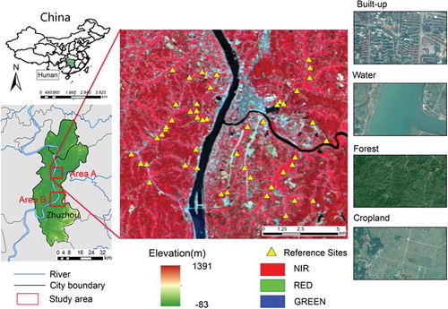
The study area is located in Zhuzhou city, Hunan province, China (Figure 1). The hilly terrain of Zhuzhou City typifies a complex landscape. The cropland is mainly distributed along both sides of the Xiangjiang River, which flows across the city from south to north. Zhuzhou is characterized by high-volume food production, primarily from cultivated paddies. According to field survey data, the paddy rice in Zhuzhou is grown annually from early June to mid-September, a period of approximately 110 days. The distribution of rice planting in Zhuzhou typifies the patchy, fragmented crop distribution of hilly regions in South China. The four major land cover categories are built-up, water, forest and cropland, where the cropland includes abandoned land and paddy rice. Because of the topography restriction and mixed landscapes, these land cover categories are difficult to distinguish.

Figure 1. Location of the study area(112°17′-114°07′E, 26°03′-28°01′N).

2.2 Data

2.2.1 Experimental data

The remote sensing data for classification were HJ-1 A/B charge-coupled device (CCD) images acquired by the Chinese Environment and Disaster Reduction Small Satellites. These data were downloaded from the China Center for Resources Satellite Data and Application (http://www.cresda.com/CN/). With their mid–high spatial resolution (30 m) and high temporal resolution (two days), CCD images are advantageous for the present study. Each CCD image consists of four channels: band 1: 0.43–0.52 μm (blue), band 2: 0.52–0.60 μm (green), band 3: 0.63–0.69 μm (red) and band 4: 0.76–0.90 μm (near-infrared). Sixteen CCD images with satisfactory data quality and within the crop growing period in 2013 were selected for classification. The acquisition times of these images are shown in Table 1. All images were pre-processed sequentially by radiometric calibration, atmospheric correction and geometric correction.

Table 1. Acquisition times of the CCD images.

Number	Date	DOY1	Number	Date	DOY1
1 2 3 4 5 6 7 8	13/Jun 17/Jun 30/Jun 08/Jul 12/Jul 25/Jul 29/Jul 07/Aug	163 167 180 188 192 205 209 218	9 10 11 12 13 14 15 16	09/Aug 11/Aug 13/Aug 25/Aug 09/Sep 15/Sep 19/Sep 21/Sep	220 222 224 236 251 261 265 267

¹Note: DOY, day of year

2.2.2 Validation data

The validation data were obtained from GF-1, high-resolution Google Earth images and field survey. The GF-1 image is the first image of the Chinese High Resolution Earth Observation System. It has a high temporal resolution (four days) and a high spatial resolution (two 2-m panchromatic/8-m multispectral cameras and four 16-m wide-field imagers). The GF-1 image consists of four channels: band 1: 0.45–0.52 μm (blue), band 2: 0.52–0.59 μm (green), band 3: 0.63–0.69 μm (red) and band 4: 0.77–0.89 μm (near-infrared). Moreover, multi-resolution (up to 0.5 m) satellite images were provided by Google Earth. Fifty validation sites (each covering several pixels and are obtained by field survey) with good visual interpretation on GF-1, Google Earth images and the field survey were selected for validation. The reference sites are indicated with yellow triangles in Figure 1.

3. Methods

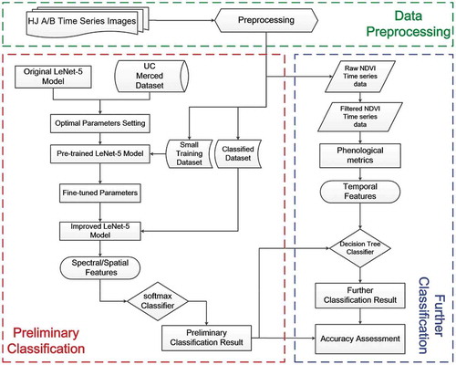
The proposed classification method includes two major steps: (1) preliminary classification of cropland, forest, buildup and water by the pre-trained CNN method; (2) further classification of paddy rice and abandoned land by the DT method (see Figure 2). The classification results of proposed method were evaluated and compared with BPNN, original CNN, and pre-trained CNN methods.

Figure 2. Flowchart of the proposed methodology.

3.1 Preliminary classification by CNN

3.1.1 Classical CNN architecture

A CNN consists of several layers with different functions: an input layer, a convolutional layer, a pool layer, a full connection layer and an output layer (Lecun et al. 1998; Tajbakhsh and Suzuki 2016). The training data are imported using the input layer, and their features are extracted with the convolutional layer. More convolution layers will add increasingly deeper features. The pool layer reduces the complexity of the whole network, and extracts the key features. The full connection layer connects all the features of the pool layer, and sends the output values for further handling. The output layer classifies the data into different categories.

Many available neural network structures include LeNet-5, AlexNet and Vgg-16 Net (Bui et al. 2011). The proper CNN architecture, rather than the CNN depth, is related to the classified image. Considering the factors of image resolution and classification object size, the classical network, LeNet-5, is selected by cross-validation. LeNet-5, a classical CNN proposed by LeCun in (1998), successfully recognizes isolated objects, and its classification is more abstract and robust than those of other common methods (Lecun et al. 1998; Tong, Li, and Zhu 2017). Considering the spatial resolution of the classified imagery and the sizes of the classified objects, we chose a LeNet-5 model for the current classification problems. The details of the LeNet-5 model are covered in Lecun et al. (1998).

3.1.2 Pre-training the LeNet-5 model using the UC merced dataset

Deep learning is advantageous because it automatically learns the efficient knowledge of the classified objects, and builds a complicated model in more difficult classification situations. However, complex models require a large amount of labeled data for training, because the depth of the structure is positively correlated with the amount of training data. If the labeled data are insufficient to support the whole training process, the deep learning model returns an unsatisfactory result. Therefore, the correct amount of training data guarantees the rationality and reliability of the training model. Traditionally, the training data are obtained through visual interpretation, which is limited and time-consuming. When the number of labeled samples is limited, the trained parameters of the CNN cannot obtain the optimal values. The data shortage problems can be solved by the so-called transfer learning method, which also reduces the training cost and avoids the overfitting problem.

Two primary transfer learning strategies are presently available for pattern recognition (including the classification of remote sensing images) (Pan and Yang 2010; Nogueira, Penatti, and Santos 2016; Pena-Barragan et al. 2011; Qian et al. 2017). The first strategy is the pre-trained model, which extracts features from small-size datasets containing high-similarity data. The CNN model trains a large dataset, and saves the optimal weight parameters for fine-tuning on the small dataset. The second strategy is the fine-tuned model, which has the same architecture as the pre-trained model. Starting from randomly initialized weight parameters, this model is retrained on the new dataset. This model is suitable for small-sized datasets containing low-similarity data (Nogueira, Penatti, and Santos 2016). The present study must analyze a small dataset of remote sensing imagery with high similarity to the pre-trained dataset. Thus, the first transfer learning strategy, based on the pre-trained model, is suitable for our purpose.

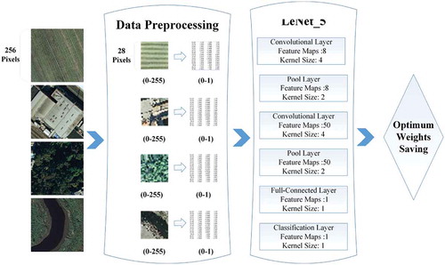
To obtain suitable weight parameters in the pre-trained dataset, a large dataset is usually required. Several remote sensing datasets, such as the UC Merced land use dataset and the NWPU-RESISC45 dataset, are available. The UC Merced dataset, downloadable from UC Merced http://vision.ucmerced.edu/, is widely used for model pre-training. The images in the UC Merced dataset have been manually extracted from large images in the USGS National Map Urban Area Imagery Collection, which maps various urban areas around the country. As the UC Merced data are similar to the classification images in the present study, they were applied as the pre-trained dataset (Avramović and Risojević 2016). The pixel resolution of this public domain imagery is one foot (0.3048 m). The dataset contains 21 classes each with 100 images. Examples of the four land classes adopted in the present study are shown in the left panel of Figure 3. The original images (RGB bands consisting of (256$\times$ 256) pixels) were resampled to (28$\times$28) pixels. The data pre-processing and pre-trained model structure is illustrated in the center and right panels of Figure 3, respectively.

Figure 3. Original images, data pre-processing and feature extraction by LeNet-5.

To circumvent the large amount of training data required for deep learning, the transfer learning mechanism sets the model parameters using a large dataset with high similarity to the analyzed data, then fine-tunes the parameters on the specific dataset, which was established manually by selecting the images from the image to be classified. Given the high correlativity between the model parameters and classification accuracy, the model parameters must be carefully selected to ensure high-quality final results. However, there are no widely-applied weight-parameter selection methods for the various classification situations. Referring to previous studies, we selected four model parameters for testing and discussion: kernel size, learning rate, batch size and activation function.

3.2 Further classification coupled with phenological metrics

3.2.1 Smoothing of the NDVI time-series data

The NDVI is correlated with the photosynthetic capacity of the vegetation, and is calculated as follows (Tucker 1979).

(1) $\mathrm{N}\mathrm{D}\mathrm{V}\mathrm{I}=\frac{\left({\rho }_{\mathrm{N}\mathrm{I}\mathrm{R}}-{\rho }_{\mathrm{R}\mathrm{E}\mathrm{D}}\right)}{\left({\rho }_{\mathrm{N}\mathrm{I}\mathrm{R}}+{\rho }_{\mathrm{R}\mathrm{E}\mathrm{D}}\right)}$(1)

where ${\rho }_{\mathrm{N}\mathrm{I}\mathrm{R}}$ and ${\rho }_{\mathrm{R}\mathrm{E}\mathrm{D}}$ are the spectral reflectance of the near-infrared and red bands, respectively. Due to cloud and atmospheric contamination, NDVI time series are generally discontinuous and noisy. Therefore, prior to the phenology extraction, the noise must be removed from the time series by a filter method (Bradley et al. 2007).

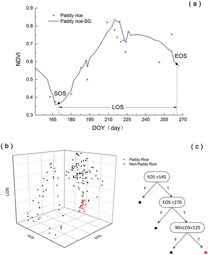
Here, the NDVI time series was smoothed by the S–G filter, named after its proposers (Chen 2004; Savitzky et al. 1964). The S–G filter, which is widely used in time series reconstruction, smooths the time series by least-squares-fitting convolution and calculates groups of adjacent values. Figure 4(a) shows an S–G filtered NDVI time-series extracted from the raw NDVI data, along with the phenological metrics.

Figure 4. Acquiring the phenological metrics of a paddy rice field.

3.2.2 Rice classification using the phenological metrics

As the phenological metrics, we selected the Start of Growing Season (SOS), End of Growing Season (EOS) and Length of Growing Season (LOS; see Figure 4). The SOS and EOS were determined as 20% of the vegetation growth and decay amplitudes, respectively, between the maximum and minimum NDVI. They were measured from the left and right minimum levels, respectively. Meanwhile, the LOS defines the time between the start and end of the growing season. These three phenological metrics can distinguish paddy rice from abandoned lands, as shown in Figure 4. They can also extract the paddy field from cropland; the latter is then classified as abandoned land. To meet this need, the classification results of the CNN method are further classified using the DT method programmed in the classification algorithms.

The DT in this paper is structured as shown in (Figure 4(b-c)). The decision nodes were determined using field survey (Liu et al. 2017). As traditional agriculture operations are inconsistent, the phenological metrics were obtained as ranges. The dates of the SOS, EOS and LOS were determined as after DOY(day of the year)$140,$ before DOY 270 and DOY 90–125, respectively.

4. Results and analysis

4.1 Determination of optimal pre-trained CNN model parameters

Figure 5(a) plots the accuracy of the models with different kernel sizes (3, 4 and 5). The accuracy was almost independent of kernel size, although the accuracy slightly improved with largest kernel size ranges between the 20th and $200\mathrm{t}\mathrm{h}$ epoch. After Epoch 200, the result of the (4 × 4) kernel gradually converged to that of the (5 × 5) kernel. To ensure high accuracy and the inclusion of the fine features during training, and considering the experimental data size, we selected the (4$\times$4) kernel for the CNN.

Figure 5. Optimizing the model parameters. Plotted are the model accuracy versus time characteristics of the CNN for different (a) kernel sizes, (b) learning rates, (c) batch sizes and (d) activity functions.

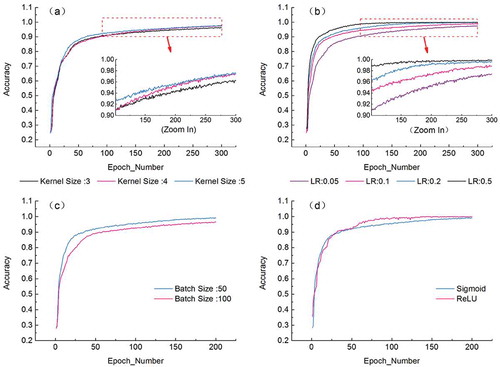
The next parameter is the learning rate (LR), which defines the learning efficiency of the CNN model. An inappropriately fast LR causes fluctuation decline in the training curve, and an mis-specified slow LR can trap the algorithm in local optima. The accuracy at different LRs are plotted in Figure 5(b) (the inset is a zoom-in of the region framed by the red dotted rectangle in the main image). After a given number of epochs, the accuracy differences among the LRs were quite small. With a sufficiently large value of epochs, the differences gradually diminished, and eventually vanished. Thus, to ensure an adequate training speed while avoiding local optima, we selected a moderate learning rate (LR = 0.2).

The batch size refers to the number of samples selected at one training time. When selecting the batch size, one usually considers the size of the dataset and the required training accuracy. As shown in Figure 5(c), reducing the batch size increases the debugging speed. Considering the size of the dataset, we set the batch size to 50 rather than 100, although other studies have shown that a large batch size reduces the vibration over a certain range of the training curve, and optimizes the convergence accuracy (Shin et al. 2016; Kovács et al. 2017).

Finally, the activation function of a node defines the output of that node for a given input or set of inputs to the computational network. An appropriately chosen activation function is critical for obtaining good training results. Owing to the simple network structure in this study, the rectified linear unit (ReLU) activation function was not remarkably superior to the sigmoid activation function (see Figure 5(d)). However, considering the short operation time, high efficiency and maintenance of the gradient characteristics, we selected the ReLU activation function. The effects of the different parameter settings on the final results are more intuitively shown in Table 2.

Table 2. Accuracy assessment of the CNN model parameters.

	Kernel Size			Learning Rate				Batch Size		Activation Function
Parameter	3	4	5	0.05	0.1	0.2	0.5	50	100	ReLU	Sig^1
Accuracy	96%	98%	97%	98%	99%	99%	99%	98%	96%	99%	98%

¹Note: sig, sig is short for sigmoid

4.2 Performance of the preliminary classification with CNN

To improve the analysis, the classification results of the original untrained and the pre-trained CNN models were compared with those of the classical BPNN method, a classical shallow ANN that has long been used in remote-sensing image classification.

BPNN is composed of three layers: input layer, output layer and hidden layer.The classical BP network model was adopted, and the parameter setting was selected according to the experimental results. In order to reflect the difference in application accuracy of the method more objectively, the training accuracy of the three models is the same 99% before the test sample verification.The classification results of the four land cover types by the three methods are shown in (Figure 6(a-c)). Additionally, the classification accuracy and their confidence intervals are presented in Table 3. These results were calculated using the accuracy assessment method proposed by Olofsson et al, (2013, 2014). This method summarized the accuracy assessment by reporting the estimated error matrix in terms of proportion of area and estimates of accuracy (Olofsson et al. 2013, 2014).

Table 3. Classification accuracy of (a) BPNN, (b) Original CNN, and (c) the pre-trained CNN.

	BPNN			Original CNN			Pre-trained CNN
Class	UA^1	PA^1	$\pm$2S^1	UA^1	PA^1	$\pm$2S^1	UA^1	PA^1	$\pm$2S^1
Cropland	0.53	0.11	0.01	0.43	0.33	0.02	0.82	0.62	0.01
Forest	0.50	0.88	0.04	0.58	0.77	0.04	0.89	0.97	0.03
Built-up	0.49	0.86	0.01	0.47	0.11	0.00	1.00	1.00	0.00
Water	0.96	0.83	0.00	0.86	0.96	0.00	1.00	0.89	0.00
OA	52.90%		0.02	55.15%		0.02	89.86%		0.02

¹Note: UA is short for user’s accuracy; PA is short for producer’s accuracy; OA is overall accuracy; $\pm$2S is the 95% confidence interval for accuracy; S is the estimated standard error of the estimated area proportion.

Figure 6. Classification results in Area A: (a) BPNN, (b) original CNN, (c) the pre-trained CNN and (d) the proposed coupling method. Classification results in Area B: (e) the pre-trained CNN and (f) the proposed coupling method. PRF: paddy rice field, AL: abandoned land.

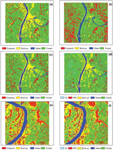
As confirmed in Figure 6(a-c), the proposed method achieved much higher classification accuracy than the two existing methods, especially in the cropland and built-up categories. As the BPNN is a shallow network, the number of network parameters in this method is relatively small, so the detailed characteristics are weakly evaluated. Meanwhile, the small training dataset in the original CNN model cannot fully train the model. Consequently, the weight parameters are incompletely trained and the accuracy requirements are not met. Owing to their poor performances, the BPNN and original CNN methods are not further considered in this manuscript. Further classification will be carried out on the results of fine-tuned CNN model and accuracy evaluation will be achieved.

4.3 Performance of further classification method coupled with phenological metrics

Figure 6(d) shows the classification results after coupling the pre-trained CNN model with the phenological metrics. The overall accuracy of the proposed coupling method was 93.56%. The five categories – paddy fields, forest, built-up, water and abandoned land – are clearly exhibited in Table 4, and the abandoned land is separated from the cropland as a new category. Forest, built-up, and water were classified more accurately than paddy fields and abandoned land. The abandoned land mainly distributes in the west of the Xiangjiang River, and the patches are highly fragmented. However, in the east of the Xiangjiang River, abandoned lands are sparse and scattered, and paddy-field patches are large and concentrated.

Table 4. Classification accuracy of the proposed coupling method.

Class	Water	Built-up	Forest	PRF	AL	Map^1	$W_i$^1	UA	PA	$\pm$2S^1
Water	1383	0	0	0	0	12,270	0.05	1.00	0.72	0.00
Built-up	0	737	0	0	0	30,407	0.13	1.00	1.00	0.00
Forest	12	0	550	22	0	161,455	0.68	0.94	0.99	0.02
PRF	28	0	24	438	59	21,300	0.09	0.80	0.64	0.00
AL	11	0	0	98	301	13,758	0.06	0.73	0.82	0.00
OA	93.56%

¹Note: PRF is short for paddy rice field, AL is short for abandoned land, map is the estimated area of each class, $W_i$ is the portion of the area mapped as category i,UA is short for user’s accuracy; PA is short for producer’s accuracy; OA is overall accuracy; $\pm$2S is the 95% confidence interval for accuracy; S is the estimated standard error of the estimated area proportion.

To further verify the effectiveness of the proposed method, we investigated a large research area. The classification results of the pre-trained CNN and the proposed method are shown in panels (e) and (f) of Figure 6, respectively. The conclusion of this supplementary experiment is consistent with that of the previous experiment. The overall accuracy of the proposed coupling method was 93.56%. Abandoned lands are mainly distributed in the west of the Xiangjiang River, as observed in area A of the previous classification, but the patches are lowly fragmented and most of the abandoned lands are located near built-up areas. In the east of the Xiangjiang River, abandoned lands are scattered and sparse, whereas the paddy-field patches are large and concentrated. Most importantly, unlike the other tested methods (the BPNN, original CNN and pre-trained CNN), the proposed method effectively separated the abandoned land from the cropland, and realized accurate rice mapping.

5. Discussion

This study proposed an efficient method for rice mapping in complex landscape regions. Deep learning and phenological metrics were combined to extract the spectral/spatial features and the temporal features of paddy fields, respectively. Coupling the deep learning and phenological metrics can effectively improve the classification accuracy of remote sensing images, especially in rice mapping and abandoned land identification.

Mapping crop area using remote sensing imagery is essential for agricultural production. However Rice is usually mapped by extracting the time-series features from MODIS data. The spatial resolution of MODIS is suitable only for analyzing large rice-growing areas, and is inadequate for analyzing rice-growing areas in complex landscapes. The present study was completed on mid-range spatial resolution data, which captured the finer features that are omitted in low-resolution data, but at lower image-acquisition cost and over a larger coverage. The mid-spatial resolution classification did not adversely compromise the precision (which exceeded 93.56%). In addition, as the rice paddies were obtained from the cropland using the time features, we also indirectly obtained the distribution of abandoned land using this method. Increasing the amount of abandoned lands may reduce the total grain production, thereby exacerbating the food crisis. By understanding the distribution and evolution of the abandoned lands, agricultural policy makers can effectively formulate their solutions.

Our method resulted in a precise paddy rice map, but several limitations remain. First, the selected CNN structure depends on the situation of the study area and the resolution of the remote sensing images. The present CNN model is optimized by adjusting the activation function and parameter settings. The method is suitable for rice mapping in complex landscape regions such as Zhuzhou, where the rice distribution is fragmented. Therefore, the CNN structure and optimal parameters require adjustment to the situation. Secondly, the accuracy of phenological metrics depends on the weather conditions. The traditional agriculture mechanism desynchronizes the phenological phases of the crops, and judgment based on empirical knowledge is inherently uncertain. Thirdly, Because of the image size difference between the pre-trained dataset (UC Merced Land Use Dataset) and the fine-tuned dataset, the pre-trained data are compressed from a dimension of 256 by 256 to 28 by 28, resulting in a certain loss of information. Due to the limitation of training data size, we pay more attention to the advantages of CNN in mining the features of image topology, and texture, the loss of color information in compression was ignored. Finally, the classification process cannot extract and use the deep characteristics of the time-series data images. To excavate the deeper information, the method must simultaneously learn the features of the time-series characteristics and the spectral/spatial characteristics.

In further work, the spectral, spatial and temporal feature extractions should be integrated into a single model. Moreover, we should also employ images with finer spectral resolution, and increase both the depth of the convolutional network and the identification precision of the mixed pixels.

6. Conclusions

We proposed an innovative method to accurately map paddy fields in complex landscapes with time-series remote sensing imagery. The method integrates a deep learning method with phenological metrics. In a series of experiments, the proposed method outperformed other state-of-the-art classification methods, achieving an overall mapping accuracy of 93.56%$\pm$ 0.01%. The proposed method demonstrated its effectiveness in paddy-mapping under complicated landscape conditions, and correctly classified abandoned lands. The method is expected to assist researchers and agricultural managers of rice mapping in complex landscape regions, and it can also provide useful information (e.g. crop yield estimates, land management decisions, land uses and cover changes) for agronomic planners.

Disclosure statement

No potential conflict of interest was reported by the authors.

Additional information

Funding

This work was supported by the National Natural Science Foundation of China Youth Science Foundation Project [Grant No. 41701387].

References

- Avramović, A., and V. Risojević. 2016. “Block-based Semantic Classification of High-resolution Multispectral Aerial Images.” Signal Image & Video Processing 10 (1): 75–84. doi:10.1007/s11760-014-0704-x.
- Bargiel, D. 2017. “A New Method for Crop Classification Combining Time Series of Radar Images and Crop Phenology Information.” Remote Sensing of Environment 198: 369–383. doi:10.1016/j.rse.2017.06.022.
- Boschetti, M. 2013. “Application of an Automatic Rice Mapping System to Extract Phenological Information from Time Series of MODIS Imagery in African Environment: First Results of Senegal Case Study.” Earsel Symposium. doi:10.5194/os-10-845-2014
- Bradley, B. A., R. W. Jacob, J. F. Hermance, and J. F. Mustard. 2007. “A Curve Fitting Procedure to Derive Inter-annual Phenologies from Time Series of Noisy Satellite NDVI Data.” Remote Sensing of Environment 106 (2): 137–145. doi:10.1016/j.rse.2006.08.002.
- Bui, H. M., M. Lech, E. Cheng, K. Neville, and I. S. Burnett. 2011. “Object Recognition Using Deep Convolutional Features Transformed by a Recursive Network Structure.” IEEE Access 4: 10059–10066. doi:10.1109/access.2016.2639543.
- Chen, J. 2004. “A Simple Method for Reconstructing A High-quality NDVI Time-series Data Set Based on the Savitzky-Golay Filter.” Remote Sensing of Environment 91 (3–4): 332–344. doi:10.1016/j.rse.2004.03.014.
- Chen, J., J. Huang, and J. Hu. 2016. “Mapping Rice Planting Areas in Southern China Using the China Environment Satellite Data.” Mathematical and Computer Modelling 54 (3–4): 1037–1043. doi:10.1016/j.mcm.2010.11.033.
- Chockalingam, J., and S. Mondal. 2017. “Fractal-Based Pattern Extraction from Time-Series NDVI Data for Feature Identification.” IEEE Journal of Selected Topics in Applied Earth Observations and Remote Sensing 10 (12): 5258–5264. doi:10.1109/jstars.2017.2748989.
- Dong, J. W., and X. M. Xiao. 2016. “Evolution of Regional to Global Paddy Rice Mapping Methods: A Review.” Isprs Journal of Photogrammetry and Remote Sensing 119: 214–227. doi:10.1016/j.isprsjprs.2016.05.010.
- Du, Z., J. Yang, C. Ou, and T. Zhang. 2019. “Smallholder Crop Area Mapped with a Semantic Segmentation Deep Learning Method.” Remote Sensing 11: 888. doi:10.3390/rs11070888.
- Feng, L., L. Zhu, H. Liu, Y. Huang, P. Du, and E. Adaku. 2015. “Urban Vegetation Classification Based on Phenology Using HJ-1A/B Time Series Imagery.” Joint Urban Remote Sensing Event (JURSE). doi:10.1109/jurse.2015.7120477.
- Gudex-Cross, D., J. Pontius, and A. Adams. 2017. “Enhanced Forest Cover Mapping Using Spectral Unmixing and Object-based Classification of Multi-temporal Landsat Imagery.” Remote Sensing of Environment 196: 193–204. doi:10.1016/j.rse.2017.05.006.
- Gumma, M. K., A. Nelson, P. S. Thenkabail, and A. N. Singh. 2011. “Mapping Rice Areas of South Asia Using MODIS Multitemporal Data.” Journal of Applied Remote Sensing 5 (1): 053547. doi:10.1117/1.3619838.
- Gumma, M. K., P. S. Thenkabail, K. C. Deevi, I. A. Mohammed, P. Teluguntla, A. Oliphant, and A. M. Whitbread. 2018. “Mapping Cropland Fallow Areas in Myanmar to Scale up Sustainable Intensification of Pulse Crops in the Farming System.” GIScience and Remote Sensing 1–24. doi:10.1080/15481603.2018.1482855.
- Hansen, M. C., and T. R. Loveland. 2012. “A Review of Large Area Monitoring of Land Cover Change Using Landsat Data.” Remote Sensing of Environment 122 (1): 66–74. doi:10.1016/j.rse.2011.08.024.
- Kim, M., J. Ko, S. Jeong, J. Yeom, and H. Kim. 2017. “Monitoring Canopy Growth and Grain Yield of Paddy Rice in South Korea by Using the GRAMI Model and High Spatial Resolution Imagery.” GIScience and Remote Sensing 54 (4): 534–551. doi:10.1080/15481603.2017.1291783.
- Kim, M., and J. Yeom. 2015. “Sensitivity of Vegetation Indices to Spatial Degradation of Rapid Eye Imagery for Paddy Rice Detection: a Case Study of South Korea.” GIScience and Remote Sensing 52 (1): 1–17. doi:10.1080/15481603.2014.1001666.
- Kontgis, C., A. Schneider, and M. Ozdogan. 2015. “Mapping Rice Paddy Extent and Intensification in the Vietnamese Mekong River Delta with Dense Time Stacks of Landsat Data.” Remote Sensing of Environment 169: 255–269. doi:10.1016/j.rse.2015.08.004.
- Kovács, G., L. Tóth, D. V. Compernolle, S. Ganapathy, G. Kovács, L. Tóth, and S. Ganapathy. 2017. “Increasing the Robustness of CNN Acoustic Models Using Autoregressive Moving Average Spectrogram Features and Channel Dropout.” Pattern Recognition Letters 100: 44–50. doi:10.1016/j.patrec.2017.09.023.
- Kumhalova, J., and S. Matejkova. 2017. “Yield Variability Prediction by Remote Sensing Sensors with Different Spatial Resolution.” International Agrophysics 31 (2): 195–202. doi:10.1515/intag-2016-0046.
- Lecun, Y., L. Bottou, Y. Bengio, and P. Haffner. 1998. “Gradient-based Learning Applied to Document Recognition.” Proceedings of the IEEE 86 (11): 2278–2324. doi:10.1109/5.726791.
- Leutheuser, H., D. Schuldhaus, and B. M. Eskofier. 2013. “Hierarchical, Multi-Sensor Based Classification of Daily Life Activities: Comparison with State-Of-the-Art Algorithms Using a Benchmark Dataset.” PloS One 8 (10): e75196. doi:10.1371/journal.pone.0075196.
- Li, D., F. Yang, and X. Wang. 2016. “Study on Ensemble Crop Information Extraction of Remote Sensing Images Based on SVM and BPNN.” Journal of the Indian Society of Remote Sensing 45 (2): 229–237. doi:10.1007/s12524-016-0597-y.
- Liao, Z., and G. Carneiro. 2017. “A Deep Convolutional Neural Network Module that Promotes Competition of Multiple-size Filters.” Pattern Recognition. doi:10.1016/j.patcog.2017.05.024.
- Liu, S., X. Liu, M. Liu, L. Wu, C. Ding, and Z. Huang. 2017. “Extraction of Rice Phenological Differences under Heavy Metal Stress Using EVI Time-Series from HJ-1A/B Data.” Sensors 17 (6): 1243. doi:10.3390/s17061243.
- Liu, Y., B. Zhang, L. Wang, and N. Wang. 2013. “A Self-trained Semisupervised SVM Approach to the Remote Sensing Land Cover Classification.” Computers and Geosciences 59 (9): 98–107. doi:10.1016/j.cageo.2013.03.024.
- McCloy, K. R., F. R. Smith, and M. R. Robinson. 1987. “Monitoring Rice Areas Using Landsat Mss Data.” International Journal of Remote Sensing 8 (5): 741–749. doi:10.1080/01431168708948685.
- Nogueira, K., O. A. B. Penatti, and J. A. D. Santos. 2016. “Towards Better Exploiting Convolutional Neural Networks for Remote Sensing Scene Classification.” Pattern Recognition 61: 539–556. doi:10.1016/j.patcog.2016.07.001.
- Olofsson, P., G. M. Foody, M. Herold, S. V. Stehman, C. E. Woodcock, and M. A. Wulder. 2014. “Good Practices for Estimating Area and Assessing Accuracy of Land Change.” Remote Sensing of Environment 148 (5): 42–57. doi:10.1016/j.rse.2014.02.015.
- Olofsson, P., G. M. Foody, S. V. Stehman, and C. E. Woodcock. 2013. “Making Better Use of Accuracy Data in Land Change Studies: Estimating Accuracy and Area and Quantifying Uncertainty Using Stratified Estimation.” Remote Sensing of Environment 129 (2): 122–131. doi:10.1016/j.rse.2012.10.031.
- Onojeghuo, A. O., G. A. Blackburn, Q. Wang, P. M. Atkinson, D. Kindred, and Y. Miao. 2018. “Rice Crop Phenology Mapping at High Spatial and Temporal Resolution Using Downscaled MODIS Time-series.” GIScience and Remote Sensing 55 (5): 659–677. doi:10.1080/15481603.2018.1423725.
- Pan, S. J., and Q. Yang. 2010. “A Survey on Transfer Learning.” IEEE Transactions on Knowledge and Data Engineering 22 (10): 1345–1359. doi:10.1109/TKDE.2009.191.
- Pena-Barragan, J. M., M. K. Ngugi, R. E. Plant, and J. Six. 2011. “Object-based Crop Identification Using Multiple Vegetation Indices, Textural Features and Crop Phenology.” Remote Sensing of Environment 115 (6): 1301–1316. doi:10.1016/j.rse.2011.01.009.
- Phiri, D., and J. Morgenroth. 2017. “Developments in Landsat Land Cover Classification Methods: A Review.” Remote Sensing 9 (9): 967. doi:10.3390/rs9090967.
- Qian, P., K. Zhao, Y. Jiang, K. H. Su, Z. Deng, S. Wang, and R. F. M. Jr. 2017. “Knowledge-leveraged Transfer Fuzzy C -means for Texture Image Segmentation with Self-adaptive Cluster Prototype Matching.” Knowledge-Based Systems 130: 33–50. doi:10.1016/j.knosys.2017.05.018.
- Qin, Y., X. Xiao, J. Dong, Y. Zhou, Z. Zhu, G. Zhang, and X. Li. 2015. “Mapping Paddy Rice Planting Area in Cold Temperate Climate Region through Analysis of Time Series Landsat 8 (OLI), Landsat 7 (ETM+) and MODIS Imagery.” Isprs Journal of Photogrammetry and Remote Sensing 105: 220–233. doi:10.1016/j.isprsjprs.2015.04.008.
- Qiu, B., D. Lu, Z. Tang, C. Chen, and F. Zou. 2017. “Automatic and Adaptive Paddy Rice Mapping Using Landsat Images: Case Study in Songnen Plain in Northeast China.” Science of the Total Environment 598: 581–592. doi:10.1016/j.scitotenv.2017.03.221.
- Qiu, B., W. Li, Z. Tang, C. Chen, and W. Qi. 2015. “Mapping Paddy Rice Areas Based on Vegetation Phenology and Surface Moisture Conditions.” Ecological Indicators 56: 79–86. doi:10.1016/j.ecolind.2015.03.039.
- Rottensteiner, F., G. Sohn, J. Jung, M. Gerke, C. Baillard, S. Benitez, and U. Breitkopf. 2012. “The Isprs Benchmark on Urban Object Classification and 3d Building Reconstruction.” International Society for Photogrammetry and Remote SensingI-3 293–298. doi:10.5194/isprsannals-I-3-293-2012.
- Rumelhart, D. E., G. E. Hinton, and R. J. Williams. 1986. “Learning Representations by Back-propagating Errors.” Nature 323 (6088): 533–536. doi:10.1038/323533a0.
- Savitzky, A., and M. J. E. Golay. 1964. “Smoothing and Differentiation of Data by Simplified Least Squares Procedures.” Analytical Chemistry 36 (8): 1627–1639. doi:10.1021/ac60214a047.
- Shin, H. C., H. R. Roth, M. Gao, L. Lu, Z. Xu, I. Nogues, and R. M. Summers. 2016. “Deep Convolutional Neural Networks for Computer-Aided Detection: CNN Architectures, Dataset Characteristics and Transfer Learning.” IEEE Transactions on Medical Imaging 35 (5): 1285–1298. doi:10.1109/tmi.2016.2528162.
- Son, N. T., C. F. Chen, C. R. Chen, H. N. Duc, and L. Y. Chang. 2013. “A Phenology-Based Classification of Time-Series MODIS Data for Rice Crop Monitoring in Mekong Delta, Vietnam.” Remote Sensing 6 (1): 135–156. doi:10.3390/rs6010135.
- Su, T. 2017. “Efficient Paddy Field Mapping Using Landsat-8 Imagery and Object-Based Image Analysis Based on Advanced Fractel Net Evolution Approach.” GIScience and Remote Sensing 54 (3): 354–380. doi:10.1080/15481603.2016.1273438.
- Tajbakhsh, N., and K. Suzuki. 2016. “Comparing Two Classes of End-to-End Machine-Learning Models in Lung Nodule Detection and Classification: MTANNs Vs. CNNs.” Pattern Recognition 63: 476–486. doi:10.1016/j.patcog.2016.09.029.
- Tong, C., J. Li, and F. Zhu. 2017. “A Convolutional Neural Network Based Method for Event Classification in Event-driven Multi-sensor Network.” Computers and Electrical Engineering 60: 90–99. doi:10.1016/j.compeleceng.2017.01.005.
- Tucker, C. J. 1979. “Red and Photographic Infrared Linear Combinations for Monitoring Vegetation.” Remote Sensing and Environment 8 (2): 127–150. doi:10.1016/0034-4257(79)90013-0.
- Wang, J., J. Huang, K. Zhang, X. Li, B. She, C. Wei, and X. Song. 2015. “Rice Fields Mapping in Fragmented Area Using Multi-Temporal HJ-1A/B CCD Images.” Remote Sensing 7 (4): 3467–3488. doi:10.3390/rs70403467.
- Wang, J., J. Huang, P. Gao, C. Wei, and L. Mansaray. 2016. “Dynamic Mapping of Rice Growth Parameters Using HJ-1 CCD Time Series Data.” Remote Sensing 8 (11): 931. doi:10.3390/rs8110931.
- Xia, G. S., J. W. Hu, F. Hu, B. G. Shi, and X. Bai. 2017. “A Benchmark Data Set for Performance Evaluation of Aerial Scene Classification.” IEEE Transactions On Geoscience And Remote Sensing 55 (7): 3965–3981. doi:10.1109/TGRS.2017.2685945.
- Xiao, X., S. Boles, J. Liu, D. Zhuang, S. Frolking, C. Li, and B. M. Iii. 2005. “Mapping Paddy Rice Agriculture in Southern China Using Multi-temporal MODIS Images.” Remote Sensing of Environment 95 (4): 480–492. doi:10.1016/j.rse.2004.12.009.
- Xiao, X., S. Boles, S. Frolking, C. Li, J. Y. Babu, W. Salas. 2006. “Mapping Paddy Rice Agriculture in South and Southeast Asia Using Multi-temporal Modis Images.” Remote Sensing of Environment 100 (1): 95–113. doi:10.1016/j.rse.2005.10.004.
- Xie, Y., Z. Sha, and M. Yu. 2008. “Remote Sensing Imagery in Vegetation Mapping: a Review.” Journal of Plant Ecology 1 (1): 9–23. doi:10.1093/jpe/rtm005.
- XU, M., P. WATANACHATURAPORN, P. VARSHNEY, and M. ARORA. 2005. “Decision Tree Regression for Soft Classification of Remote Sensing Data.” Remote Sensing of Environment 97 (3): 322–336. doi:10.1016/j.rse.2005.05.008.
- Yang, M. D., K. S. Huang, Y. H. Kuo, T. Hui, and L. M. Lin. 2017. “Spatial and Spectral Hybrid Image Classification for Rice Lodging Assessment through UAV Imagery.” Remote Sensing 9 (6): 583. doi:10.3390/rs9060583.
- Yang, Y., and S. Newsam 2010. “Bag-of-visual-words and Spatial Extensions for Land-use Classification.” Proceedings of the 18th SIGSPATIAL International Conference on Advances in Geographic Information Systems - GIS ’10, ACM, New York, USA, 270–279. doi:10.1145/1869790.1869829.
- Yue, J., W. Zhao, S. Mao, and H. Liu. 2015. “Spectral–spatial Classification of Hyperspectral Images Using Deep Convolutional Neural Networks.” Remote Sensing Letters 6 (6): 468–477. doi:10.1080/2150704x.2015.1047045.
- Zhang, C., Y. Han, F. Li, S. Gao, D. Song, H. Zhao, K. Fan, and Y. Zhang. 2019. “A New CNN-Bayesian Model for Extracting Improved Winter Wheat Spatial Distribution from GF-2 Imagery.” Remote Sensing 11 (6). doi:10.3390/rs11060619.
- Zhang, G., X. Xiao, J. Dong, W. Kou, C. Jin, Y. Qin, and C. Biradar. 2015. “Mapping Paddy Rice Planting Areas through Time Series Analysis of MODIS Land Surface Temperature and Vegetation Index Data.” Isprs Journal of Photogrammetry and Remote Sensing 106: 157–171. doi:10.1016/j.isprsjprs.2015.05.011.
- Zhang, H., Q. Li, J. Liu, J. Sshang, X. Du, L. Zhao, and T. Dong. 2017. “Crop Classification and Acreage Estimation in North Korea Using Phenology Features.” GIScience and Remote Sensing 54 (3): 381–406. doi:10.1080/15481603.2016.1276255.