A hyperspectral experiment over tropical forests based on the EO-1 orbit change and PROSAIL simulation

ABSTRACT

We designed a unique hyperspectral experiment from the Earth Observing One (EO-1) orbit change to evaluate solar illumination effects over tropical forests in Brazil. Ten nadir-viewing Hyperion images collected over a fixed site and period of the year (July to August) were selected for analysis. We evaluated variations in reflectance and in 16 narrowband vegetation indices (VIs) with increasing solar zenith angle (SZA) from the pre-drift (2004–2008) to the EO-1 drift period (2011–2016). To detect changes in reflectance and shadows, we applied spectral mixture analysis (SMA) and principal component analysis (PCA) and calculated the similarity spectral angle (θ) between the vegetation spectra measured with variable SZA. The magnitude of the illumination effects was also evaluated from change-point analysis and nonparametric Mann-Whitney U tests applied over the time series. Finally, we complemented our experiment using the PROSAIL model to simulate the VIs variation with increasing SZA resultant from satellite drift. The results showed significant changes in Hyperion reflectance and VIs, especially when the EO-1 crossed the study area at earlier times and larger SZA in 2015 (9:05 a.m.; SZA = 59°) and 2016 (8:30 a.m.; SZA = 67°). Compared to the pre-drift period (10:30 a.m.; SZA = 45°), the SZA differences of 14° (2015) and 22° (2016) increased the shade fractions and decreased the vegetation brightness. PCA separated the pre-drift and drift reflectance datasets, showing shifts in scores due to changes in brightness. θ increased with SZA, indicating changes in the shape of the vegetation spectra with drift. For most VIs, the change-point analysis indicated 2015 (SZA = 59°) as the predominant year of detected changes. Compared to the EO-1 original orbit, the Plant Senescence Reflectance Index (PSRI), Anthocyanin Reflectance Index (ARI) and Structure Insensitive Pigment Index (SIPI) presented the largest positive changes during drift, while the Photochemical Reflectance Index (PRI), Visible Atmospherically Resistant Index (VARI) and Enhanced Vegetation Index (EVI) had the largest negative changes. The effect size of the illumination geometry on these VIs was large, as indicated by increasing values of the Cohen’s r metric toward 2016. The anisotropy of the Hyperion VIs was generally consistent with that from PROSAIL in the simulated pre-drift and drift periods. Focusing on structural indices, it affected the relationships between VIs and simulated leaf area index (LAI) at large SZA.

KEYWORDS:

• EO-1
• Hyperion
• orbit change
• solar illumination effects
• tropical forests
• Amazon
• hyperspectral
• vegetation indices

1. Introduction

Improved measurements from the upcoming hyperspectral missions will provide great amounts of datasets for large areas of the Earth (e.g. the Environmental Mapping and Analysis Program (EnMAP) described by Guanter et al. 2015). Such measurements bring new perspectives for investigating a variety of ecosystem processes in tropical forests of the Amazon (Hilker et al. 2017; Kokaly et al. 2009). For instance, depending on the ability to remove the confounding effects of vegetation structure on the hyperspectral signal, canopy chemical attributes can be estimated from these satellites (Asner et al. 2015). In addition, analysis of narrowband vegetation indices (VIs) can determine other properties associated with vegetation structure and plant physiology (Cuba et al. 2018; Roberts, Roth, and Perroy 2012). When combined with the spectral-temporal information provided by tower-mounted hyperspectral cameras in the Amazon, satellite-derived narrowband VIs can improve knowledge of vegetation phenology (de Moura et al. 2017). This is important for a better comprehension of the climate sensitivity of tropical forests.

Narrowband VIs are based on well-described physical principles. However, VIs are generally affected by the geometry of data acquisition, especially when determined from large field-of-view (FOV) sensors or instruments with pointing capability. The effects are wavelength dependent and vary in magnitude with vegetation canopy structure and composition (land cover); FOV; pointing angle; local topography (terrain illumination); site location, time and period of data acquisition (solar illumination) (Galvão et al. 2013, 2016; Maeda and Galvão 2015). While the angular sensitivity of several narrowband VIs has been described before (Verrelst et al. 2008), less attention has been given in the literature to solar illumination effects.

The investigation of solar illumination effects over tropical forests is important for different reasons. For instance, the amplitude in solar zenith angle (SZA) reaches values of 18° during the dry season of southern Amazon, which affects, to some extent, the behavior of some VIs calculated from near-polar orbiting satellites (Galvão et al. 2011). Furthermore, the launching of equatorial-orbit satellites has been considered as an alternative to increase the chances of acquiring cloud-free data over the Amazon. Using a low equatorial orbit, we can obtain high temporal resolution data (five images a day) from 5° N to 15° S of latitude with spatial resolution ranging from 40 m at nadir to 200 m at extreme viewing (Kono et al. 2003). By acquiring data at two-hour spaced intervals, significant changes in illumination conditions will be observed every day and seasonally for a given pixel having a fixed view angle. Finally, compared to polar-orbiting satellites, complementary information for vegetation monitoring can be obtained at coarse spatial resolution from diurnal VI observations from geostationary satellites (Fensholt et al. 2006). An example is the multispectral Advanced Baseline Imager (ABI) on the Geostationary Operational Environmental Satellite (GOES-R).

In satellite studies of vegetation phenology over the Amazon, diurnal variations in narrowband VIs can be seen as a noise in the time series to be further compensated by Bidirectional Reflectance Distribution Function (BRDF) models, or as a source of information to be further explored. In both cases, the sensitivity of the different narrowband VIs to solar illumination effects should be better understood. To address this problem, analysis of the impacts of orbit drift on reflectance time series can be useful, as demonstrated in previous studies with the Advanced Very High Resolution Radiometer (AVHRR) or Landsat sensors (e.g. Lindstrom et al. 2006; Nagol et al. 2015; Privette et al. 1995; Tucker et al. 2005; Zhang and Roy 2016)

The Earth Observing-One (EO-1) satellite, launched on 21 November 2000, was decommissioned in 2017 after completing more than 16 years of operation. The Hyperion, onboard the EO-1, was the first orbital hyperspectral instrument acquiring data in 196 calibrated bands (10 nm of bandwidth) between 400 and 2400 nm with a spatial resolution of 30 m, swath width of 7.7 km and a revisit time of 16 days (Pearlman et al. 2003). In 2008, the EO-1 orbit was slightly lowered in approximately 5 km in relation to the Landsat 7’s orbit. In February 2011, the satellite ran out of the fuel necessary to maintain orbit, as described in detail by Franks et al. (2017). As a result, there was a change in precession rate (satellite orbit drift) that produced increasingly earlier equatorial crossing times from 2011 until the end of the mission.

The effects of orbit change on satellite overpass time depend on the site location and are stronger at higher latitudes (Franks et al. 2017). In southern Amazon, the EO-1 overpass time changed from approximately 10:30 a.m. in the pre-drift period to 8:30 a.m. in the drift period, producing SZA variations in July-August from 45° (pre-drift) to 67° (drift period) across the years. During the Hyperion data acquisition, greater amounts of shadows were captured by the sensor after the change in precession rate from 2011 to 2016. However, in spite of the expected decrease in signal-to-noise ratio (SNR) with increasing SZA, no marked trend in decreasing quality in Hyperion was apparent through 2016 (Franks et al. 2017). Because of the preservation of data quality through the end of the mission, the available time series of Hyperion data can constitute nice experiments to be further explored in solar illumination investigations. Consequently, even during the orbit change at the end of the mission, the Hyperion/EO-1 was still useful for science applications, providing very interesting data at variable SZA for selected sites in the world.

In the present study, we evaluated for the first time solar illumination effects on hyperspectral data. We designed a unique hyperspectral experiment from the EO-1 satellite drift to analyze solar illumination effects on Hyperion reflectance and 16 narrowband VIs measured over seasonal evergreen forest from southern Amazon. Using 10 nadir-viewing Hyperion images acquired between 2004 and 2016 over a fixed site and period of the year (July to August), we reduced the seasonal influences of SZA and of vegetation phenology on the analysis, while highlighted the solar illumination effects derived solely from the EO-1 orbit change. To complement the analysis of this experiment, we used the PROSAIL radiative transfer model to simulate computationally the VIs variations over the evergreen forest with increasing SZA resultant from satellite drift.

2. Methodology

2.1. Hyperion data acquisition and pre-processing

The study area comprises a preserved fragment (8 x 4 km) of seasonal evergreen forest having an average tree height of 17.13 ± 1.30 m, basal area of 14.31 ± 2.52 m²/ha and emergent sparse trees of 30 m height. The study area is located close to the Xingu Indigenous Park, in the Brazilian state of Mato Grosso (central coordinates = S 13°12ʹ22” and W 52°20ʹ59”). Because the local topography is flat, terrain illumination or topographic effects are not observed there.

In Brazil, like in other parts of the world, it is very difficult to find a dense time series of Hyperion data. However, over the study area, Hyperion collected many images in nadir and off-nadir viewing. From the available set of images, in order to reduce the view angle influence on results, we selected 10 cloud-free scenes acquired at nadir viewing (≤10° of pointing angle) in a short period of each year (20 July to 11 August) (Table 1). This period is coincident with the local dry season. The selection of this window time interval was necessary to reduce the seasonal SZA effects on the data analysis. From the list of images in Table 1, Hyperion data, acquired between 2004 and 2008, comprised the regular period of data acquisition (pre-drift). Data acquired between 2011 and 2016 corresponded to the EO-1 drift period. From 2008 to 2010, a slight modification in orbit was registered, as discussed in the previous section.

Table 1. Attributes of the selected set of nadir-viewing Hyperion/EO-1 images acquired in the pre-drift (2004–2008) and EO-1 orbit change periods (2011–2016). Data from 2010 were obtained under a slight modification in orbit compared to the Landsat-7 orbit. Negative and positive pointing angles indicate backscattering and forward scattering directions, respectively.

Date of Hyperion image acquisition	Pointing angle (°)	EO-1 orbit status	Solar zenith angle (SZA)	Local time of satellite overpass (a.m.)
8 August 2004	+9	pre-drift	42°	10:28
27 July 2005	+9	pre-drift	45°	10:28
2 August 2006	−10	pre-drift	46°	10:19
22 July 2008	−1	pre-drift	47°	10:21
22 July 2010	+5	orbit lowered	46°	10:24
24 July 2011	−6	drift	47°	10:18
20 July 2013	0	drift	51°	10:00
29 July 2014	−10	drift	55°	9:32
10 August 2015	−1	drift	59°	9:05
11 August 2016	+6	drift	67°	8:30

Image preprocessing included the use of an algorithm to reduce striping effects (Goodenough et al. 2003). The atmospheric correction converted the at-sensor radiance from the 196 calibrated Hyperion bands into surface reflectance images. The Fast Line-of-Sight Atmospheric Analysis of Spectral Hypercubes (FLAASH) removed atmospheric scattering and absorption effects using a MODTRAN-based approach (Harris Geospatial Solutions, Inc., Melbourne, Florida). Model parameters included a tropical atmosphere with a rural aerosol. Initial estimates of visibility were performed using the 2-Band (K–T) method (Kaufman et al. 1997). To estimate precipitable water vapor on a per-pixel basis, we used the 1130-nm spectral feature. The FLAASH polishing algorithm removed spectral artifacts resultant from atmospheric correction. After atmospheric correction, we excluded 44 noisy bands associated with intervals of strong water vapor absorption (1400 and 1900 nm) and left 152 bands positioned between 427 nm and 2355 nm in the analysis.

2.2. Data analysis

2.2.1. Solar illumination effects on reflectance

We investigated solar illumination effects on Hyperion reflectance. First, the effects of change in the EO-1 original orbit to modify the amounts of shadows viewed by the sensor over seasonal evergreen forest were evaluated using linear spectral mixture analysis (SMA). SMA assumes that the reflectance of each pixel is a linear combination of the endmember reflectance values (van der Meer 2004). A three-endmember model (green vegetation, soil, and shade) was considered in the analysis. Candidate endmembers for green vegetation and soil were extracted for each pre-drift image (2004–2008) using the Sequential Maximum Angle Convex Cone (SMACC) approach (Gruninger, Ratkowski, and Hoke 2004). SMACC uses residual minimization to find pixels with contrasting brightness in the scene. The process is repeated until a user-defined number of endmembers is reached or when a pixel already detected is captured again. After final selection of the green vegetation and soil endmembers from spectra inspection of the different pre-drift dates, we chose a spectrally flat low reflectance spectrum to represent the shade endmember (Roberts, Smith, and Adams 1993). Using a fixed set of three endmembers, we generated fraction images and inspected them over time for detecting variations in shade with increasing SZA resultant from satellite drift.

In the second step of the data analysis, we randomly selected 500 pixels for each date of image acquisition over the homogeneous evergreen forest to reduce spatial autocorrelation. This number of pixels ensured confidence in the data analysis, especially for principal component analysis (PCA), considering the great number of Hyperion bands. We applied PCA to the reflectance of 5000 pixels (500 per date) to detect the Hyperion bands responsible for most of the data variance in the time series. The first two components having the largest eigenvalues were extracted. The contribution of each band to explain each principal component was determined from the component matrix values. Reflectance variations in seasonal evergreen forest due to earlier EO-1 satellite overpasses were evaluated from scatterplots of the first two PC scores.

The last step in reflectance data analysis was just to reduce brightness variations detected by PCA while highlighting possible modifications in the shape of the spectra produced by increasing SZA toward 2016. For this purpose, we obtained an average reflectance spectrum (reference) representing the pre-drift period (2004–2008; 500 pixels versus four dates; total of 2000 pixels) and calculated the similarity spectral angle (θ) for each date and pixel selected before. θ varies with changes in the shape of the spectra rather than with changes in brightness. It is the same metric adopted in the Spectral Angle Mapper (SAM) classification. The equation used in the calculation of θ is found in several works (e.g. Kruse et al. 1993; Adeline et al. 2018).

2.2.2. Solar illumination effects on hyperspectral vegetation indices

We selected 16 narrowband VIs with spectral variations associated with canopy structure, biochemistry, and physiology (Roberts, Roth, and Perroy 2012). The selected VIs, abbreviations, equations and references are listed in Table 2. Using the average response of pixels selected before (500 per date), we generated temporal profiles for each VI and compared the VI behavior in the pre-drift and drift periods of the EO-1 satellite.

Table 2. Selected Hyperion vegetation indices (VIs) associated with canopy structure, biochemistry, and physiology. The VI classification is based on Roberts, Roth, and Perroy (2012). ρ is the reflectance. The original equations were adapted to the closest Hyperion bands.

Vegetation index	Equation	Reference
	Structure
Enhanced Vegetation Index (EVI)	2.5 × ((ρ864nm − ρ660nm)/(ρ864nm + 6 × ρ660nm − 7.5 × ρ467nm + 1))	Huete et al. (2002)
Enhanced Vegetation Index 2 (EVI2)	2.5 × ((ρ864nm − ρ660nm)/(ρ864nm + 2.4 × ρ660nm + 1))	Jiang et al. (2008)
Normalized Difference Vegetation Index (NDVI)	(ρ864nm − ρ660nm)/(ρ864nm + ρ660nm)	Rouse et al. (1973)
Visible Atmospherically Resistant Index (VARI)	(ρ559nm − ρ660nm)/(ρ559nm + ρ660nm – ρ487nm)	Gitelson et al. (2002)
Visible Index Green (VIG)	(ρ559nm − ρ660nm)/(ρ559nm + ρ660nm)	Gitelson et al. (2002)
	Biochemistry
Anthocyanin Reflectance Index (ARI)	(1/ρ559nm) − (1/ρ721nm)	Gitelson et al. (2002)
Leaf Water Vegetation Index 2 (LWVI2)	(ρ1094nm – ρ1205nm)/(ρ1094nm + ρ1205nm)	Galvão, Formaggio, and Tisot (2005)
Moisture Stress Index (MSI)	ρ1598nm/ρ823nm	Hunt and Rock (1989)
Normalized Difference Infrared Index (NDII)	(ρ823nm − ρ1649nm)/(ρ823nm + ρ1649nm)	Hunt and Rock (1989)
Normalized Difference Water Index (NDWI)	(ρ854nm − ρ1245nm)/(ρ854nm + ρ1245nm)	Gao (1996)
Pigment Specific Simple Ratio (PSSR)	ρ803nm/ρ671nm	Blackburn (1998)
Plant Senescence Reflectance Index (PSRI)	(ρ681nm – ρ498nm)/ρ752nm	Merzlyak et al. (1999)
Structure Insensitive Pigment Index (SIPI)	(ρ803nm − ρ467nm)/(ρ803nm + ρ681nm)	Peñuelas, Baret, and Filella (1995)
Water Band Index (WBI)	ρ905nm/ρ972nm	Peñuelas et al. (1997)
	Physiology
Photochemical Reflectance Index (PRI)	(ρ529nm − ρ569nm)/(ρ529nm + ρ569nm)	Gamon, Serrano, and Surfus (1997)
Red Edge NDVI (RENDVI)	(ρ752nm − ρ701nm)/(ρ752nm + ρ701nm)	Gitelson, Merzlyak, and Lichtenthaler (1996)

To determine statistically whether changes occurred in the VI time series as well as their periods of occurrence, we applied change-point analysis. The change point model (CPM) package written in R (R Development Core Team) was used. This analysis provides an effective and computationally efficient method for detecting multiple change-points in Gaussian and non-Gaussian sequences (Ross 2015). After testing the data distribution for normality, we chose the nonparametric Mann-Whitney U statistics (α = 0.05) in the change-point analysis for detecting the year when the changes occurred.

Finally, to determine the most sensitive narrowband VIs to solar illumination effects, we obtained for each VI the relative change between the median of 2016 (n = 500 pixels), when the largest SZA was locally observed, and the median of the pre-drift period (2004–2008) (n = 2000 pixels). Because the scale differences between the VIs could affect the percentage changes, we also computed for each VI the effect size of the EO-1 satellite drift over the regular period of data acquisition. We tested whether the median values differed between the pre-drift period (averaged between 2004 and 2008) and each year of change in the original orbit of the satellite (2011–2016). To describe the relevant magnitude of solar illumination effects over the VI determination, we calculated Cohen’s r metric of effect size from the Mann-Whitney U values (Cohen 1988).

2.2.3. PROSAIL simulations

We complemented the Hyperion experiment using the PROSAIL model. We simulated the response of each VI over the evergreen forest as a function of the SZA range observed during the EO-1 orbit drift (45° to 67°). PROSAIL integrates the leaf radiative transfer PROSPECT with the canopy radiative transfer SAIL (Scattering by Arbitrary Inclined Leaves) (Jacquemoud et al. 2009). It is one of the most widely used and validated models in temperate and dense tropical ecosystems (Hilker et al. 2017).

The major input parameters used to simulate the Hyperion VIs of the seasonal evergreen forest are listed in Table 3. The Leaf Area Index (LAI) of five was defined from the MOD15A2 (MODIS/Terra Leaf Area Index/FPAR 8-Day L4 Global 1 km) product. The definition of the biochemical attributes was based on vegetation chlorophyll estimates in the Amazon provided by Hilker et al. (2017), who reported also some measured values of this constituent in leaves.

Table 3. Major input parameters used in the PROSAIL simulations to retrieve the directional reflectance of seasonal evergreen forest as a function of leaf area index (LAI) and solar zenith angle (SZA).

Variable	Description	Unit	Value
Cab	Chlorophyll content	µg.cm^−2	45
Car	Carotenoid content	µg.cm^−2	10
CBrown	Brown pigment content	µg.cm^−2	0.1
Cw	Leaf equivalent water thickness	cm	0.02
Cm	Leaf dry matter content	g.cm^−2	0.009
N	Structure coefficient		1.5
LAI	Leaf area index		5
LAD	Leaf angle distribution	m^2 m^−2	Hemispheric
Sc	Soil coefficient		1
SZA	Solar zenith angle	Degree	0 to 70
VZA	View zenith angle	Degree	0 (nadir)
RAA	Relative azimuth angle	Degree	0

Finally, because LAI did not vary significantly over the forest, as indicated by the MOD15A2 product and available measurements of the Plant Area Index (PAI) (Galvão et al. 2011), we used PROSAIL to simulate changes in this biophysical parameter. We correlated PROSAIL-simulated LAI values (1 to 5 in steps of 0.1) with two commonly used structural VIs listed in Table 2 (NDVI and EVI), as a function of the SZA of the pre-drift (45°) and extreme drift (67°) periods of Hyperion/EO-1 data acquisition.

3. Results

3.1. Solar illumination effects on Hyperion reflectance

From inspection of the Hyperion metadata, we observed in the study area a significant decrease in the local time of satellite overpass with changes in the EO-1 original orbit (Table 1). When compared to the pre-drift time (10:30 a.m.), the overpass time decreased from 15 minutes, in 2011, to two hours (8:30 a.m.), in 2016. As a result, the SZA increased during the Hyperion data acquisition from an average value of 45° (pre-drift; 2004–2008) to 47° (2011), 51° (2013), 55° (2014), 59° (2015) and 67° (2016) (Table 1). No significant changes were observed between 2008 and 2011 from the slight EO-1 deorbit, which was approximately 5 km lower than the Landsat 7 orbit.

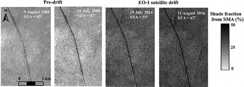
Because of the decrease in local time of EO-1 overpass and the resultant increase in SZA, the Hyperion captured greater amounts of shadows during the drift period of data acquisition. In false-color composites using the Hyperion bands centered at 864 nm (red), 1648 nm (green) and 660 nm (blue), darker reddish shades were observed over the seasonal evergreen forest with increasing SZA (Figure 1). From the SMA, preceded by the use of the SMACC approach to select endmembers (location indicated in Figure 1), we obtained average shade fractions from a three-endmember model (green vegetation, soil, and shade). The shade fractions ranged from 14.3 ± 4.9% in 2004 before drift to 32.2 ± 8.7% in 2016 during drifting (Figure 2).

Figure 1. Brightness changes in Hyperion/EO-1 false-color composites from the pre-drift and drift periods of hyperspectral image acquisition. The location of the study area in southern Amazon and of the SMACC-detected green vegetation (GV) and soil endmembers in the scene are indicated.

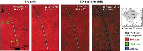
Figure 2. Shade fractions derived from spectral mixture analysis (SMA) for the pre-drift and drift periods of satellite data acquisition. The amounts of shadows, captured by the Hyperion over seasonal evergreen forest, increased with increasing solar zenith angle (SZA) toward 2016.

The spectral modifications from EO-1 orbit change were also observed when PCA was applied to the Hyperion reflectance of pixels from the 10 different dates (500 pixels per date). Using the Bartlett Test of sphericity, we rejected the null hypothesis that the correlation matrix was an identity matrix, excluding the possibility of a population with zero correlation (p-value < 0.001). The Kaiser-Meyer-Olkin measure of 0.996 indicated sampling adequacy for PCA. Most of the data variance was concentrated over the first two components (60%) with their PC scores separating the pre-drift Hyperion datasets (green color in Figure 3) from the drift datasets (blue and red colors). The most significant spectral changes in the PC space were observed in 2015 and 2016, when the EO-1 satellite crossed the study area at earlier times (9:05 and 8:30 a.m., respectively) and at larger SZA (59° and 67°, respectively). Surprisingly, PCA captured also variations in Hyperion reflectance in 2010 (cyan color in Figure 3), when the EO-1 orbit was slightly lowered in relation to the Landsat 7 orbit.

Figure 3. Projection of the first two scores from principal component analysis (PCA) applied to the reflectance of 152 Hyperion bands (427–2355 nm), as a function of the EO-1 orbit change. Results refer to 5000 pixels (500 per date) extracted over the seasonal evergreen forest.

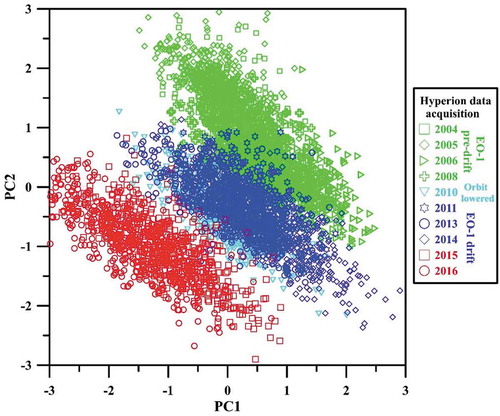
From the pre-drift (2004–2008) to the drift (2011–2016) periods, PC scores shifted toward the left side of PC1 and toward the bottom of PC2 with increasing solar illumination effects (Figure 3). In PC1, this shifting was a measure of brightness, as expressed by large correlations (loadings) between the reflectance of the Hyperion bands from the visible, near-infrared (NIR) and shortwave infrared (SWIR-1) intervals (426–1790 nm) and the PC1 scores (results not shown). Therefore, brightness (mean reflectance in the 426–1790 nm range) decreased with increasing shadows in the drift period, as expected. The matrix component loadings of PC2 reproduced an inverted vegetation spectrum in the visible and NIR intervals, expressing variations in relative differences between their reflectance (results not shown). Thus, while the first most important source of data variance (47% for PC1) detected by PCA was vegetation brightness, the second one was the reflectance difference between the visible and NIR bands (13% for PC2).

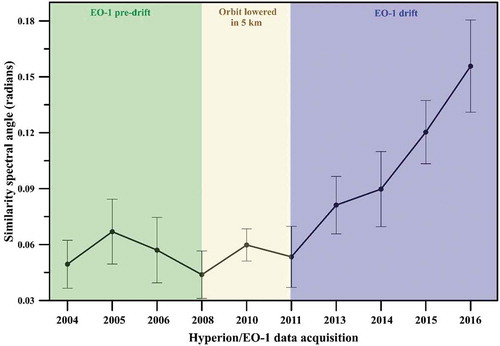
Inspection of the Hyperion spectra of seasonal evergreen forest (average of 500 pixels per date), before and after orbit change, confirmed the reflectance decrease over time detected by PCA (Figure 4). Modifications in the shape of the vegetation spectra with satellite drift were also apparent in these spectra, including the visible interval. We quantified such modifications by calculating the similarity spectral angle (θ) between the reference spectrum (mean reflectance in the 2004–2008 period) and the reflectance curves of each year in the time series. Compared to the pre-drift reference spectrum, the greatest changes in the shape of the reflectance curves were observed in the drift period, especially in 2015 and 2016 (Figure 5). From the Mann-Whitney U tests, the spectral angle differences between these two years and the other pre-drift years in the time series were significant at the 0.05 statistical level.

Figure 4. Hyperion average reflectance spectra of seasonal evergreen forest representative of the pre-drift and drift periods of the EO-1 satellite (n = 500 pixels per date). Spectra from other years were omitted for a better graphic representation.

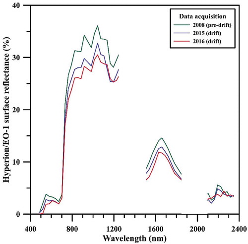
Figure 5. Variation in mean spectral similarity angle (θ) for comparison of the similarity in the shape of the Hyperion spectra of seasonal evergreen forest, before and after the EO-1 orbit change. θ was calculated using the average pre-drift spectrum (2004–2008; n = 2000 pixels) as a reference and reflectance values of the 500 pixels from each date as a test of comparison. The standard deviation bars are indicated.

3.2. Solar illumination effects on Hyperion vegetation indices

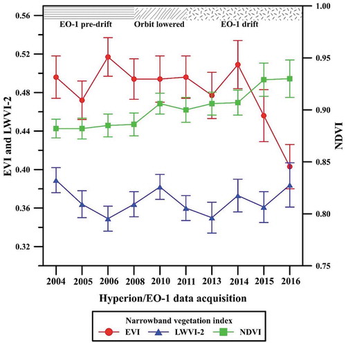
We detected three types of VI behavior with solar illumination effects (Figure 6). From the narrowband VIs listed in Table 2, the Anthocyanin Reflectance Index (ARI), Normalized Difference Vegetation Index (NDVI), Plant Senescence Reflectance Index (PSRI), Pigment Specific Simple Ratio (PSSR), Red-Edge NDVI (RENDVI) and Structure Insensitive Pigment Index (SIPI) increased with the EO-1 orbit changes at large SZA in 2015 and 2016. On the other hand, the Enhanced Vegetation Index (EVI), Enhanced Vegetation Index-2 (EVI2), Photochemical Reflectance Index (PRI), Visible Atmospherically Resistant Index (VARI) and Visible Index Green (VIG) decreased with great amounts of shadows captured by the Hyperion at earlier times of satellite overpass. Finally, the Leaf Water Vegetation Index-2 (LWVI-2), Moisture Stress Index (MSI), Normalized Difference Infrared Index (NDII), Normalized Difference Water Index (NDWI) and Water Band Index (WBI) did not present well-defined trends with solar illumination effects. In general, the most sensitive indices to solar illumination effects were VIs calculated from NIR-visible or visible-visible Hyperion bands or those that were not mathematically normalized in their formulations. VIs determined from NIR-SWIR Hyperion bands (MSI and NDII) or from bands located close to leaf/canopy water absorption features (NDWI, LWVI-2, and WBI) had less sensitivity to such effects.

Figure 6. Examples of three behaviors of Hyperion vegetation indices. Average values increased for NDVI and decreased for EVI at larger solar zenith angles (SZA) in 2015 and 2016. LWVI-2 was less sensitive to solar illumination effects derived from changes in the EO-1 satellite orbit (top of figure).

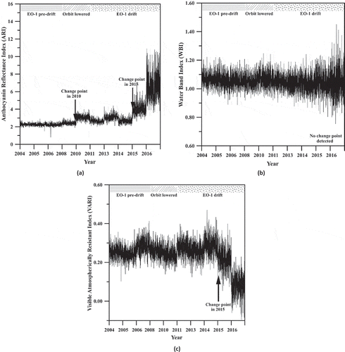
Results from the change-point analysis at 0.05 level of statistical significance detected 2015 as the predominant year of VI change due to orbit drift (Table 4). Examples of detected and non-detected changes are presented in Figure 7(a–c). In 2015, the SZA was 59° and the local time of satellite overpass was 9:05 a.m. The EO-1 overpass was therefore approximately one hour and half earlier than the regular time of data acquisition (10:30 a.m.) (Table 1). In addition to changes detected in 2015, the change-point analysis captured also a second point of change in 2010 only for very few VIs (e.g. ARI in Figure 7(a)). This detection may be associated with the slight deorbit of the EO-1 satellite in relation to the Landsat 7 orbit, which requires further investigations. Brightness changes in 2010, outside the period of drift, were also detected from PCA (Figure 3).

Table 4. Change-point analysis in the period of EO-1 orbit drift (2011–2016), indicating the detected year in the time series of Hyperion vegetation indices (VI). Results are statistically significant (α = 0.05). The VI abbreviations are defined in Table 2.

VI	ARI	EVI	EVI2	LWVI-2	MSI	NDII	NDVI	NDWI	PRI	PSRI	PSSR	RENDVI	SIPI	VARI	VIG	WBI
Year	2015	2015	2016	-	-	-	2015	-	2015	2015	2015	2015	2015	2015	2014	-

Figure 7. Change-point analysis for (a) ARI (positive change), (b) WBI (no change) and (c) VARI (negative change), as a function of the pre-drift and EO-1 drift periods (top of figure). The changes in 2015 are associated with solar illumination effects over seasonal evergreen forest and are statistically significant (α = 0.05). In (a), a second point of change was detected in 2010 and may be associated with the slight EO-1 deorbit described in the text.

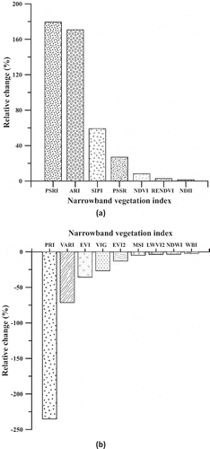
From the determination of the relative changes between the medians of the pre-drift period (2004–2008) and 2016, the year when the EO-1 satellite crossed the study area at 8:30 a.m. under a large SZA (67°), we detected the most sensitive VIs to solar illumination effects. The largest positive changes were observed for PSRI, ARI, and SIPI (Figure 8(a)), while the largest negative changes were verified for PRI, VARI, and EVI (Figure 8(b)).

Figure 8. (a) Positive and (b) negative percentage changes in medians for Hyperion narrowband vegetation indices during the earlier EO-1 overpass in 2016 (SZA = 67°), in relation to the pre-drift period (2004–2008).

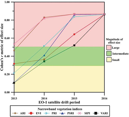
The VIs analysis of the effect size of the EO-1 satellite drift over the regular period of data acquisition confirmed the results of Figure 8. The analysis showed increasing Cohen’s r metric values toward the end of the drift period in 2016 for ARI, EVI, PRI, PSRI, SIPI and VARI (Figure 9). Using the classification scheme proposed by Cohen (1988) to evaluate the magnitude of the effect size, results indicated large solar illumination effects in 2015 and 2016 for most VIs, which was consistent with previous results. For VIs like ARI and SIPI, the effects were large earlier in 2014, when the SZA difference to the pre-drift period was 10°.

Figure 9. Variation in Cohen’s r metric of effect size (absolute values), computed from non-parametric Mann-Whitney U tests, during the period of EO-1 orbit change. The magnitude of solar illumination effects over seasonal evergreen forest is indicated by colors for selected Hyperion vegetation indices. Results for 2011 were omitted for a better graphical representation.

3.3. PROSAIL simulation of the VIs response in the pre-drift and drift periods

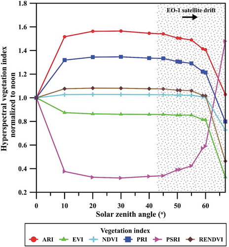
Examples of the VIs response with increasing SZA from the pre-drift to the drift periods of satellite data acquisition are shown in Figure 10. In agreement with previous Hyperion analyses, PROSAIL observations, normalized to the noon (SZA = 0°), indicated ARI, PRI, PSRI and EVI as the more anisotropic VIs for the simulated LAI of the seasonal evergreen forest of the study area. In Figure 10, the less anisotropic VIs were NDVI and RENDVI. On the other hand, when compared to Hyperion results, some divergences were also observed for some VIs at extreme SZA. For instance, the Hyperion NDVI increased at extreme SZA in the EO-1 drift period as expected from the literature (Figure 6), while the PROSAIL NDVI showed a decrease at 67° SZA due to signal saturation in the red band and to decreasing NIR reflectance.

Figure 10. PROSAIL-simulated response of selected vegetation indices with increasing solar zenith angle (SZA) from the pre-drift to the drift periods of Hyperion/EO-1 data acquisition. Results are normalized to noon (SZA = 0°). The SZA variation in July to August due to orbit change is indicated.

Solar illumination apparently affects the relationships between structural VIs and LAI at large SZA, as demonstrated by PROSAIL results (Table 5). Compared to the NDVI, the more anisotropic and non-normalized EVI showed greater variations in the coefficient of determination (R²) values at the simulated drift period of Hyperion/EO-1 data acquisition.

Table 5. Relationships between two structural vegetation indices (NDVI and EVI) and leaf area index (LAI), simulated from PROSAIL, for solar zenith angle (SZA) from the pre-drift (45°) and drift (67°) periods of Hyperion/EO-1 data acquisition. Power functions were used for fitting the data.

	EVI		NDVI
Statistical parameter	45°	67°	45°	67°
R^2	0.92	0.34	0.84	0.64
Residual mean square	0.001	0.015	0.001	0.003
n	41	41	41	41
Sig.	<0.001	<0.001	<0.001	<0.001

4. Discussion

The EO-1 satellite was decommissioned in 2017 after completing more than 16 years of operation and providing many lessons for future hyperspectral missions (Franks et al. 2017; Middleton et al. 2013). The current hyperspectral experiment from the EO-1 orbit change is inserted in this context. This is the first hyperspectral experiment addressing solar illumination effects on 16 narrowband VIs from satellite orbit change. This experiment is unique when keeping the seasonal influence of SZA and vegetation phenology approximately constant while varying illumination effects derived solely from changing times of satellite overpass (variable SZA). Complemented by PROSAIL simulations, we demonstrated the anisotropy of some VIs with changes in SZA. Based on this anisotropy, our findings indicated the possibility of using diurnal VI signatures acquired, for instance, by low equatorial orbit satellites, to obtain information on canopy structure of tropical forests. This is important in studies for discriminating mature forests from different stages of secondary successions.

In general, nearly all studied VIs showed some degree of sensitivity to solar illumination effects. From the PCA, SMA and spectral similarity angle evaluations, we observed also that such effects decreased the vegetation brightness, increased the shade fraction and modified the shape of the vegetation spectra, respectively. As indicated by the change-point analysis, significant changes over the VIs were observed when the EO-1 crossed the study area at earlier times and larger SZA in 2015 (9:05 a.m.; SZA = 59°) and 2016 (8:30 a.m.; SZA = 67°). When compared to the pre-drift period (10:30 a.m.; SZA = 45°), the most sensitive VIs to SZA were PSRI, ARI, and SIPI, which presented significant increase over time. VIs that strongly decreased with satellite drift were PRI, VARI and EVI. Overall, VIs calculated from NIR/visible and visible/visible Hyperion bands, or VIs non-normalized in their formulations, were more sensitive to solar illumination than the NIR/SWIR or NIR/NIR indices associated with leaf/canopy water or vegetation moisture (LWVI-2, MSI, NDII, NDWI, and WBI). While part of this behavior can be attributed to the difficulties of atmospheric correction in early morning observations, consistent changes over time were also observed at the initial stages of orbit change, in 2013 and 2014, when the SZA values were 51° and 55°, thus 6° and 10° greater than the observed angle in the pre-drift period (SZA = 45°).

The narrowband VI behavior with SZA observed in our study area was generally consistent with few available studies on view-illumination effects. For instance, using Hyperion data acquired during the dry season of 2005, Galvão et al. (2013) indicated PRI and EVI as the two more anisotropic VIs over tropical forests. In a view angle study using multi-angular/hyperspectral data from the Compact High-Resolution Imaging Spectrometer (CHRIS/PROBA) acquired over coniferous forests from Switzerland, Verrelst et al. (2008) found SIPI, PRI, and ARI as the most sensitive VIs to view zenith angle (VZA). The influence factors on the anisotropy of these light use efficiency and leaf pigment indices, as well as the confounding effects on canopy signal, were discussed by them. Shadow’s effects prevailed in the PRI response, while the relative proportions of green and nonphotosynthetic vegetation viewed by the sensor affected the angular behavior of SIPI and ARI.

For traditional VIs such as the NDVI and EVI, our results confirmed also earlier observations using broadband imaging sensors or field spectrometers. In our study, the Hyperion NDVI increased at large SZA because of the greater reflectance decrease observed in the red than in the NIR (Epiphanio and Huete 1995; Gao et al. 2002; Goodin, Gao, and Henebry 2004; Huete et al. 1992; Middleton 1991; Zhang and Roy 2016). The EVI decreased at large SZA following the NIR band behavior because of the greater NIR reflectance dependence of this index (Galvão et al. 2011; de Moura et al. 2017). Therefore, both VIs were sensitive to shadows, but with different levels of magnitude and trend, as was also observed by Bhandari, Phinn, and Gill (2011) using Moderate Resolution Imaging Spectroradiometer (MODIS) data.

Compared to the EO-1 pre-drift period (SZA = 45°), the differences of 14° and 22° observed in 2015 (SZA = 59°) and 2016 (SZA = 67°), respectively, produced statistically significant changes for most Hyperion VIs, especially for ARI, EVI, PRI, PSRI, SIPI, and VARI. This result has implications for other studies with different sensors and orbits. For instance, variations in SZA during the dry season of southern Amazon are even higher than 14° for images acquired by MODIS (Galvão et al. 2011). In this region, the illumination effects should be disentangled from the vegetation phenological signal by using BRDF models. This is important for the upcoming hyperspectral missions such as the EnMAP. Furthermore, over the 27 years of Landsat-5 operation, the orbit changed by nearly one hour in specific years, producing modifications in SZA greater than 10° during image acquisition. Therefore, the comparison of certain years of Landsat 5 data may result in significant reflectance and NDVI differences produced solely by the Landsat-5 orbit changes (Zhang and Roy 2016). Our findings showed that such differences depend on the vegetation index used in the data analysis. The seasonal analysis of high spatial (3.7 m) and high temporal (daily) resolution data acquired by the PlanetScope constellation of satellites should also consider SZA as a source of variability. Depending on the location of the site and vegetation type, the canopy shadow effects will be also more apparent for this type of data, including those acquired by cameras onboard the Unmanned Aerial Vehicles (UAV).

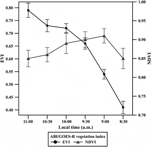
In the analysis of data acquired by near-polar orbiting satellites having large FOV instruments (e.g. MODIS), directional and VZA effects are more important than SZA effects. Different from VZA, SZA exhibits a seasonal cycle having an amplitude that increases with latitude (Franks et al. 2017; Nagol et al. 2015). In contrast, in the analysis of data acquired by geostationary satellites (e.g. ABI/GOES-R), diurnal reflectance variations for a given pixel having a fixed VZA are mainly controlled by changes in SZA. An example of these changes is presented in Figure 11 for the NDVI and EVI calculated from the broad bands of the ABI/GOES-R instrument. The data were acquired over the seasonal evergreen forest of the Xingu Indigenous Park. This park is distant 60 km west of the study area, has the same vegetation type and is composed of a lesser fragmented landscape than that observed in the vicinities of our site. Therefore, this park is adequate as a reference of comparison, considering the coarse spatial resolution of the ABI. The spatial resolution is 1 km for the blue and NIR bands and 500 m for the red band. When compared to the Hyperion results of Figure 6, we observed a concordant behavior of the ABI-derived EVI and NDVI profiles toward the early morning observations. In Figure 11, the ABI EVI decreased with increasing SZA from 11:00 a.m. to 8:30 a.m., showing changes of 48% between the morning observations. Except for the ABI data acquisition at the beginning of the morning (8:30 a.m.), the overall NDVI increase observed toward the early ABI observations, from 11:00 a.m. to 9:00 a.m., was also consistent with our findings using Hyperion data. In another study, Fensholt et al. (2006) evaluated diurnal variations in NDVI from the Spinning Enhanced Visible and Infrared Imager (SEVIRI)/Meteosat-8 sensor. For vegetated surfaces, their results were generally consistent with our patterns of increasing NDVI with earlier local times of EO-1 overpass in 2015 and 2016.

Figure 11. Morning variations (8 July 2018) in average EVI and NDVI (n = 10 pixels), calculated from ABI/GOES-R data. The data were acquired over seasonal evergreen forests from the Xingu Indigenous Park, which is distant 60 km west of the study area.

When considered as a noise in time series of hyperspectral VIs, differences in sun-sensor geometry can be normalized to a fixed geometry using BRDF correction. However, these procedures have been generally restricted to multispectral sensors (Hilker et al. 2017; Verrelst et al. 2008). When considered as a source of information, illumination effects are potentially useful for several applications. For instance, combined measurements from mid-morning and mid-afternoon acquisitions have improved the relationships between PRI and photosynthetic light use efficiency (LUE) (Middleton et al. 2016). Diurnal variations in PRI, a typical hyperspectral index that has been adapted to MODIS bands, can therefore contribute to a better detection of vegetation physiological processes in the Amazon. Our Hyperion and PROSAIL results confirmed that PRI was very anisotropic with SZA. In addition, diurnal variations of VIs can serve as a source of information on canopy structure, as demonstrated in a field reflectance experiment over crops performed by Ishihara et al. (2015). As indicated by our PROSAIL results, the SZA probably affects the estimates of biophysical attributes, depending on the anisotropy of the structural VI used in the analysis.

Finally, our study has some constraints in both analyses (Hyperion and PROSAIL). From the PROSAIL simulation, there are obvious difficulties in modeling the vertical canopy structure of the evergreen forest and in defining precisely its biophysical and biochemical parameters. In addition, the performance of the simulation apparently decreases at extreme SZA.

From the Hyperion data analysis, four important limitations should be highlighted. First, we did not investigate the land-cover type dependence of the illumination effects from the EO-1 orbit change because similar time series were not found in other parts of Brazil. Second, we assumed the 21-day window interval for image selection across years as sufficient to reduce the impact of vegetation phenology in the analysis. In the study area, PAI and canopy openness, estimated from hemispherical photographs, do not change significantly in this window interval (Galvão et al. 2011). Third, differences in pointing angles and view direction for Hyperion data acquisition introduce data variability in the analysis, but we tried to reduce this interference keeping the angles lower than 10° during image selection. Finally, the evaluation of the EO-1 orbit changes to modify the SWIR-2 reflectance (2032–2355 nm) was affected to some extent by the poor SNR of the Hyperion. The instrumental SNR added also uncertainties in atmospheric correction, especially at large SZA. However, the uncertainties produced by EO-1 orbit change in data quality and atmospheric correction were evaluated by Franks et al. (2017). They used two pseudo-invariant calibration sites over deserts from the USA (Rail Road Valley Playa) and Libya (Libya-4 site). Over the Rail Road Valley Playa site, differences in surface reflectance of the Hyperion bands ranged from 5% to 9% when compared to the mean spectral response prior drift. Over the Libya-4 pseudo-invariant calibration site, Franks et al. (2017) tested the performance of three methods of atmospheric correction, including FLAASH. They demonstrated the stability of the Hyperion data between the pre-drift and drift periods, independent of the method used for atmospheric correction. Therefore, their findings showed the high quality of the Hyperion data through the end of the mission, which were adequate in our solar illumination study.

5. Conclusions

Results from the EO-1 orbit change demonstrated the anisotropy of the VIs to solar illumination effects. Compared to the pre-drift period (2004–2008) of data acquisition (local overpass time = 10:30 a.m.; SZA = 45°), our results showed significant variations in Hyperion reflectance and VIs during the EO-1 orbit change (2011–2016). This was especially valid when the EO-1 satellite crossed the study area at earlier times and under larger SZA in 2015 (9:05 a.m.; SZA = 59°) and 2016 (8:30 a.m.; SZA = 67°), producing SZA differences of 14° and 22°, respectively. Although much lesser intense than in these two years, solar illumination effects in 2013 and 2014, with SZA differences of 6° and 10°, respectively, were still captured by PCA. From the pre-drift to the drift period, we observed modifications in vegetation brightness and in the shape of the spectra derived from greater amounts of canopy shadows captured by Hyperion at earlier times of satellite overpass.

For most VIs, the predominant year of changes detected by the change-point analysis was 2015. Compared to the EO-1 original orbit, the largest positive changes during drift were observed for PSRI, ARI, and SIPI, while the largest negative changes were verified for PRI, VARI and EVI. The magnitude of the illumination effects for ARI, EVI, PRI, PSRI, SIPI, and VARI was large during the EO-1 drift, as deduced also from increasing Cohen’s r metric values of the effect size toward 2016. The overall behavior of the VIs observed in the EO-1 orbit change experiment was generally consistent with PROSAIL simulations, which showed ARI, PRI, PSRI, and EVI as the more anisotropic VIs to solar illumination effects. The anisotropy probably affects the relationships between structural VIs and LAI at large SZA, but further studies with field-based measurements are required to confirm the magnitude of these effects with different land cover types.

Acknowledgements

The authors are grateful to the Conselho Nacional de Desenvolvimento Científico e Tecnológico (CNPq) (grant numbers 301486/2017-4 and 113769/2018-0). Mission Extension by the EO-1 Science Team was highly appreciated. Comments and suggestions by the anonymous reviewers were also highly appreciated.

Disclosure statement

No potential conflict of interest was reported by the authors.

Additional information

Funding

This work was supported by the Conselho Nacional de Desenvolvimento Científico e Tecnológico [301486/2017-4].

References

- Adeline, K. R. M., X. Briottet, X. Ceamanos, T. Dartigalongue, and J. P. Gastellu-Etchegorry. 2018. “ICARE-VEG: A 3D Physics-based Atmospheric Correction Method for Tree Shadows in Urban Areas.” ISPRS Journal of Photogrammetry and Remote Sensing 142: 311–327. doi:10.1016/j.isprsjprs.2018.05.015.
- Asner, G. P., R. E. Martin, C. B. Anderson, and D. E. Knapp. 2015. “Quantifying Forest Canopy Traits: Imaging Spectroscopy versus Field Survey.” Remote Sensing of Environment 158: 15–27. doi:10.1016/j.rse.2014.11.011.
- Bhandari, S., S. Phinn, and T. Gill. 2011. “Assessing Viewing and Illumination Geometry Effects on the MODIS Vegetation Index (MOD13Q1) Time Series: Implications for Monitoring Phenology and Disturbances in Forest Communities in Queensland, Australia.” International Journal of Remote Sensing 32: 7513–7538. doi: 10.1080/01431161.2010.524675.
- Blackburn, G. A. 1998. “Spectral Indices for Estimating Photosynthetic Pigment Concentrations: A Test Using Senescent Tree Leaves.” International Journal of Remote Sensing 19: 657–675. doi: 10.1080/014311698215919.
- Cohen, J. 1988. Statistical Power Analysis for the Behavioral Sciences. 2nd Auflage ed. Hillsdale, NJ: Erlbaum.
- Cuba, N., D. Lawrence, J. Rogan, and C. A. Williams. 2018. “Local Variability in the Timing and Intensity of Tropical Dry Forest Deciduousness Is Explained by Differences in Forest Stand Age.” GIScience & Remote Sensing 55: 437–456. doi: 10.1080/15481603.2017.1403136.
- de Moura, Y. M., L. S. Galvão, T. Hilker, J. Wu, S. Saleska, C. H. Do Amaral, B. W. Nelson, et al. 2017. “Spectral Analysis of Amazon Canopy Phenology during the Dry Season Using a Tower Hyperspectral Camera and MODIS Observations.” ISPRS Journal of Photogrammetry and Remote Sensing 131: 52–64. doi: 10.1016/j.isprsjprs.2017.07.006.
- Epiphanio, J. N., and A. R. Huete. 1995. “Dependence of NDVI and SAVI on Sun/sensor Geometry and Its Effect on fAPAR Relationships in Alfalfa.” Remote Sensing of Environment 51: 351–360. doi: 10.1016/0034-4257(94)00110-9.
- Fensholt, R., I. Sandholt, S. Stisen, and C. Tucker. 2006. “Vegetation Monitoring with the Geostationary Meteosat Second Generation SEVIRI Sensor.” Remote Sensing of Environment 101: 212–229. doi: 10.1016/j.rse.2005.11.013.
- Franks, S., C. Neigh, P. K. Campbell, G. Sun, T. Yao, Q. Zhang, K. F. Huemmrich, E. M. Middleton, S. G. Ungar, and S. W. Frye. 2017. “EO-1 Data Quality and Sensor Stability with Changing Orbital Precession at the End of a 16 Year Mission.” Remote Sensing 9: 412. doi: 10.3390/rs9050412.
- Galvão, L. S., F. M. Breunig, J. R. Dos Santos, and Y. M. de Moura. 2013. “View-illumination Effects on Hyperspectral Vegetation Indices in the Amazonian Tropical Forest.” International Journal of Applied Earth Observation and Geoinformation 21: 291–300. doi: 10.1016/j.jag.2012.07.005.
- Galvao, L. S., F. M. Breunig, T. S. Teles, W. Gaida, and R. Balbinot. 2016. “Investigation of Terrain Illumination Effects on Vegetation Indices and VI-derived Phenological Metrics in Subtropical Deciduous Forests.” GIScience & Remote Sensing 53: 360–381. doi: 10.1080/15481603.2015.1134140.
- Galvão, L. S., J. R. Dos Santos, D. A. Roberts, F. M. Breunig, M. Toomey, and Y. M. de Moura. 2011. “On Intra-annual EVI Variability in the Dry Season of Tropical Forest: A Case Study with MODIS and Hyperspectral Data.” Remote Sensing of Environment 115: 2350–2359. doi: 10.1016/j.rse.2011.04.035.
- Galvão, L. S., A. R. Formaggio, and D. A. Tisot. 2005. “Discrimination of Sugarcane Varieties in Southeastern Brazil with EO-1 Hyperion Data.” Remote Sensing of Environment 94: 523–534. doi: 10.1016/j.rse.2004.11.012.
- Gamon, J. A., L. Serrano, and J. S. Surfus. 1997. “The Photochemical Reflectance Index: An Optical Indicator of Photosynthetic Radiation-use Efficiency across Species, Functional Types, and Nutrient Levels.” Oecologia 112: 492–501. doi: 10.1007/s004420050337.
- Gao, B. 1996. “A Normalized Difference Water Index for Remote Sensing of Vegetation Liquid Water from Space.” Remote Sensing of Environment 58: 257–266. doi: 10.1016/S0034-4257(96)00067-3.
- Gao, F., Y. Jin, C. B. Schaaf, and A. H. Strahler. 2002. “Bidirectional NDVI and Atmospherically Resistant BRDF Inversion for Vegetation Canopy.” IEEE Transactions on Geoscience and Remote Sensing 40: 1269–1278. doi: 10.1109/TGRS.2002.800241.
- Gitelson, A. A., Y. J. Kaufman, R. Stark, and D. Rundquist. 2002. “Novel Algorithms for Remote Estimation of Vegetation Fraction.” Remote Sensing of Environment 80: 76–87. doi: 10.1016/S0034-4257(01)00289-9.
- Gitelson, A. A., M. N. Merzlyak, and H. K. Lichtenthaler. 1996. “Detection of Red Edge Position and Chlorophyll Content by Reflectance Measurements near 700 Nm.” Journal of Plant Physiology 148: 501–508. doi: 10.1016/S0176-1617(96)80285-9.
- Goodenough, D. G., A. Dyk, O. Niemann, J. S. Pearlman, H. Chen, and T. Han. 2003. “Processing Hyperion and ALI for Forest Classification.” IEEE Transactions on Geoscience and Remote Sensing 41: 1321–1331. doi: 10.1109/TGRS.2003.813214.
- Goodin, D. G., J. Gao, and G. M. Henebry. 2004. “The Effect of Solar Illumination Angle and Sensor View Angle on Observed Patterns of Spatial Structure in Tallgrass Prairie.” IEEE Transactions on Geoscience and Remote Sensing 42: 154–165. doi: 10.1109/TGRS.2003.815674.
- Gruninger, J., A. J. Ratkowski, and M. L. Hoke. 2004. “The Sequential Maximum Angle Convex Cone (SMACC) Endmember Model.” Proceedings of the Society of Photo-optical Instrumentation Engineers (SPIE) 5425: 1–14.
- Guanter, L., H. Kaufmann, K. Segl, S. Foerster, C. Rogass, S. Chabrillat, T. Küster, et al. 2015. “The EnMAP Spaceborne Imaging Spectroscopy Mission for Earth Observation”. Remote Sensing 7: 8830–8857. doi: 10.3390/rs70708830.
- Hilker, T., L. S. Galvão, L. E. O. C. Aragão, Y. M. de Moura, C. H. Do Amaral, A. I. Lyapustin, W. Jin, et al. 2017. “Vegetation Chlorophyll Estimates in the Amazon from Multi-angle MODIS Observations and Canopy Reflectance Model.” International Journal of Applied Earth Observation and Geoinformation 58: 278–287. doi: 10.1016/j.jag.2017.01.014.
- Huete, A., K. Didan, T. Miura, E. P. Rodriguez, X. Gao, and L. G. Ferreira. 2002. “Overview of the Radiometric and Biophysical Performance of the MODIS Vegetation Indices.” Remote Sensing of Environment 83: 195–213. doi: 10.1016/S0034-4257(02)00096-2.
- Huete, A. R., G. Hua, J. Qi, A. Chehbouni, and W. J. D. van Leeuwen. 1992. “Normalization of Multidirectional Red and NIR Reflectance with the SAVI.” Remote Sensing of Environment 41: 143–154. doi: 10.1016/0034-4257(92)90074-T.
- Hunt, E. R., and B. N. Rock. 1989. “Detection of Changes in Leaf-water Content Using near Infrared and Middle-infrared Reflectances.” Remote Sensing of Environment 30: 43–54. doi: 10.1016/0034-4257(89)90046-1.
- Ishihara, M., Y. Inoue, K. Ono, M. Shimizu, and S. Matsuura. 2015. “The Impact of Sunlight Conditions on the Consistency of Vegetation Indices in Croplands—Effective Usage of Vegetation Indices from Continuous Ground-based Spectral Measurements.” Remote Sensing 7: 14079–14098. doi: 10.3390/rs71014079.
- Jacquemoud, S., W. Verhoef, F. Baret, C. Bacour, P. J. Zarco-Tejada, G. P. Asner, C. François, and S. L. Ustin. 2009. “PROSPECT+SAIL Models: A Review of Use for Vegetation Characterization.” Remote Sensing of Environment 113 (S1): 56–66. doi: 10.1016/j.rse.2008.01.026.
- Jiang, Z. Y., A. R. Huete, K. Didan, and T. Miura. 2008. “Development of a Two-Band Enhanced Vegetation Index without a Blue Band.” Remote Sensing of Environment 112: 3833–3845. doi: 10.1016/j.rse.2008.06.006.
- Kaufman, Y. J., D. Tanré, L. A. Remer, E. F. Vermote, A. Chu, and B. N. Holben. 1997. “Operational Remote Sensing of Tropospheric Aerosol over Land from EOS Moderate Resolution Imaging Spectroradiometer.” Journal of Geophysical Research 102: 17051–17067. doi: 10.1029/96JD03988.
- Kokaly, R. F., G. P. Asner, S. V. Ollinger, M. E. Martin, and C. A. Wessman. 2009. “Characterizing Canopy Biochemistry from Imaging Spectroscopy and Its Application to Ecosystem Studies.” Remote Sensing of Environment 113: S78–S91. doi: 10.1016/j.rse.2008.10.018.
- Kono, J., M. Quintino, B. Rudorff, and H. Carvalho. 2003. “The Amazon Rainforest Monitoring Satellite – SSR-1.” Acta Astronauta 52: 701–708. doi: 10.1016/S0094-5765(03)00040-7.
- Kruse, F. A., A. B. Lefkoff, J. W. Boardman, K. B. Heidebrecht, A. T. Shapiro, P. J. Barloon, and A. F. H. Goetz. 1993. “The Spectral Image Processing System (sips)—Interactive Visualization and Analysis of Imaging Spectrometer Data.” Remote Sensing of Environment 44: 145–163. doi: 10.1016/0034-4257(93)90013-N.
- Lindstrom, J., L. Eklundh, J. Holst, and U. Holst. 2006. “Influence of Solar Zenith Angles on Observed Trends in the NOAA/NASA 8-km Pathfinder Normalized Difference Vegetation Index over the African Sahel.” International Journal of Remote Sensing 27: 1973–1991. doi: 10.1080/01431160500380539.
- Maeda, E. E., and L. S. Galvão. 2015. “Sun-sensor Geometry Effects on Vegetation Index Anomalies in the Amazon Rainforest.” GIScience & Remote Sensing 52: 332–343. doi: 10.1080/15481603.2015.1038428.
- Merzlyak, M. N., A. A. Gitelson, O. B. Chivkunova, and V. Y. U. Rakitin. 1999. “Non-destructive Optical Detection of Pigment Changes during Leaf Senescence and Fruit Ripening.” Physiologia Plantarum 106: 135–141. doi: 10.1034/j.1399-3054.1999.106119.x.
- Middleton, E. M. 1991. “Solar Zenith Angle Effects on Vegetation Indices in Tallgrass Prairie.” Remote Sensing of Environment 38: 45–62. doi: 10.1016/0034-4257(91)90071-D.
- Middleton, E. M., K. F. Huemmrich, D. R. Landis, T. A. Black, A. G. Barr, and J. H. McCaughey. 2016. “Photosynthetic Efficiency of Northern Forest Ecosystems Using a MODIS-derived Photochemical Reflectance Index (PRI).” Remote Sensing of Environment 187: 345–366. doi: 10.1016/j.rse.2016.10.021.
- Middleton, E. M., S. G. Ungar, D. J. Mandl, L. Ong, S. W. Frye, P. E. Campbell, D. R. Landis, J. P. Young, and N. H. Pollack. 2013. “The Earth Observing One (EO-1) Satellite Mission: Over a Decade in Space.” IEEE Journal of Selected Topics in Applied Earth Observations and Remote Sensing 6: 243–256. doi: 10.1109/JSTARS.2013.2249496.
- Nagol, J. R., J. O. Sexton, D. H. Kim, A. Anand, D. Morton, E. Vermote, and J. R. Townshend. 2015. “Bidirectional Effects in Landsat Reflectance Estimates: Is There a Problem to Solve?” ISPRS Journal of Photogrammetry and Remote Sensing 103: 129–135. doi: 10.1016/j.isprsjprs.2014.09.006.
- Pearlman, J. S., P. S. Barry, C. C. Segal, J. Shepanski, D. Beiso, and S. L. Carman. 2003. “Hyperion, a Space-based Imaging Spectrometer.” IEEE Transactions on Geoscience and Remote Sensing 41: 1160–1173. doi: 10.1109/TGRS.2003.815018.
- Peñuelas, J., F. Baret, and I. Filella. 1995. “Semiempirical Indexes to Assess Carotenoids Chlorophyll-a Ratio from Leaf Spectral Reflectance.” Photosynthetica 31: 221–230.
- Peñuelas, J., J. Pinol, R. Ogaya, and I. Lilella. 1997. “Estimation of Plant Water Content by the Reflectance Water Index WI (R900/R970).” International Journal of Remote Sensing 18: 2869–2875. doi: 10.1080/014311697217396.
- Privette, J. L., C. Fowler, G. A. Wick, D. Baldwin, and W. J. Emery. 1995. “Effects of Orbital Drift on Advanced Very High Resolution Radiometer Products: Normalized Difference Vegetation Index and Sea Surface Temperature.” Remote Sensing of Environment 53: 164–171. doi: 10.1016/0034-4257(95)00083-D.
- Roberts, D. A., K. L. Roth, and R. L. Perroy. 2012. “Hyperspectral Vegetation Indices.” In Hyperspectral Remote Sensing of Vegetation, edited by P. S. Thenkabail, J. G. Lyon, and A. Huete, 309–327. Boca Raton, FL: CRC Press, Taylor and Francis Group.
- Roberts, D. A., M. O. Smith, and J. B. Adams. 1993. “Green Vegetation, Nonphotosynthetic Vegetation, and Soils in AVIRIS Data.” Remote Sensing of Environment 44: 255–269. doi: 10.1016/0034-4257(93)90020-X.
- Ross, G. J. 2015. “Parametric and Nonparametric Sequential Change Detection in R: The Cpm Package.” Journal of Statistical Software 66: 1–20.
- Rouse, J. W., R. H. Haas, J. A. Schell, and D. W. Deering. 1973. “Monitoring Vegetation Systems in the Great Plains with ERTS.” Paper presented at the Third ERTS-1 Symposium, Washington, DC, December 10–14. ( NASA SP-351, vol. 1, pp. 309–317).
- Tucker, C. J., J. E. Pinzon, M. E. Brown, D. A. Slayback, E. W. Pak, R. Mahoney, E. F. Vermote, and N. El Saleous. 2005. “An Extended AVHRR 8-km NDVI Dataset Compatible with MODIS and SPOT Vegetation NDVI Data.” International Journal of Remote Sensing 26: 4485–4498. doi: 10.1080/01431160500168686.
- van der Meer, F. 2004. “Analysis of Spectral Absorption Features in Hyperspectral Imagery.” International Journal of Applied Earth Observation and Geoinformation 5 (1): 55–68. doi: 10.1016/j.jag.2003.09.001.
- Verrelst, J., M. E. Schaepman, B. Koetz, and M. Kneubuehler. 2008. “Angular Sensitivity Analysis of Vegetation Indices Derived from CHRIS/PROBA Data.” Remote Sensing of Environment 112: 2341–2353. doi: 10.1016/j.rse.2007.11.001.
- Zhang, H. K., and D. P. Roy. 2016. “Landsat 5 Thematic Mapper Reflectance and NDVI 27-year Time Series Inconsistencies Due to Satellite Orbit Change.” Remote Sensing of Environment 186: 217–233. doi: 10.1016/j.rse.2016.08.022.