Big geospatial data analysis for Canada’s Air Pollutant Emissions Inventory (APEI): using google earth engine to estimate particulate matter from exposed mine disturbance areas

ABSTRACT

Particulate Matter (PM) emissions originating from mine waste and mine tailings can be hazardous to human health, depending on the ore type and processes used to extract ore. Until now, only a single, simple estimate of the total area of mine waste area across all of Canada has been available for calculating air quality emissions from this source. This single estimate, based on manual satellite interpretation completed in 1977, was extrapolated to estimate mine areas for all years from 1990 to the present. These area estimates were used annually to calculate the particulate matter from mines for the Canadian Air Pollutant Emissions Inventory (APEI); however, there is high uncertainty in these measurements of mine area and therefore in emissions estimates. In order to increase certainty in emissions estimates, the exposed mine waste areas must be mapped for each year. Mapping mine waste over areas as large as the Canadian landmass requires enormous quantities of data and considerable computational power, which will be compounded when a time-series analysis is required. Therefore, in this study, we have employed Google Earth Engine (GEE) Javascript API to map exposed mine areas in four “benchmark” years (1990, 2000, 2010, and current year 2018) as part of the APEI. A random forest classifier was trained using two separate datasets (Landsat-5 year 2000; and a combination of Landsat-8, Sentinel-1, and Sentinel-2 for the year 2018). Transfer learning was then used to apply the year 2000 model to the year 1990 and 2010 Landsat-5 imagery, which produced classification results for the four “benchmark” years in our time series. This tool has enabled the monitoring of mine growth over a 30-year period and has confirmed that overall the area of mines is growing in Canada. Overall, Google Earth Engine proved to be an invaluable tool in mapping exposed mine waste areas and would be similarly useful for any organization with large-area monitoring mandates or those interested in time-series analysis of the Landsat archive.

KEYWORDS:

• Google Earth Engine
• random forest classification
• transfer learning
• air quality
• mine mapping

Introduction

Particulate Matter (PM) refers to airborne particles in either liquid or dust form and long-term exposure may cause adverse health effects (Hinds 1999; Pumlee and Morman 2011). PM can also affect vegetation and structures, and contribute to reduced visibility and regional haze (Environment and Climate Change Canada (ECCC) 2013a). As a result, particulate matter is one of the six air pollutants regulated under the Canadian Ambient Air Quality Standards (Environment and Climate Change Canada (ECCC) 2013b) and other similar air quality standards internationally. PM emissions originating from mine waste and mine tailings can be hazardous to human health, depending on the ore type and processes used to extract ore (e.g. Corriveau et al. 2011). The transportation of dust and aerosols through winds can be a significant problem at mine sites because of the mobility of the smaller suspended particulates. The transport of particulate matter not only occurs when the mines are in operation, but the resuspension of abandoned mine waste deposits can also occur and could be an important source of air pollution (Ekosse et al. 2004; Chopin and Alloway 2007; López, González, and Romero 2008). As tailings ponds dry, tailings that were deposited in the ponds can become windborne and therefore monitoring the changes in mine extent as well as tailing pond extents is important for predicting air pollution from mines. Therefore, the specific temporal condition of the exposed area of mine waste is an important factor for understanding the air pollutant emissions that could be produced from a mine site.

The Pollutant Inventories and Reporting Division (PIRD) of Environment and Climate Change Canada (ECCC) produces estimates of air quality emissions on an annual basis in the Air Pollutant Emission Inventory (APEI) report. The APEI is used by modelers at ECCC to produce air quality reports and alerts which are important for public health (Environment and Climate Change Canada (ECCC) 2019). The latest publication of the APEI report tracks air pollutant emissions trends from 1990 to 2017 (Environment and Climate Change Canada (ECCC) 2019). One of the emissions categories tallied in the inventory is a particulate matter from “exposed mine disturbance areas,” which includes mine tailings, tailings ponds, and waste rock. The calculation of the area of exposed mine disturbance is a computationally challenging spatial problem given the large extent of the Canadian landmass and compounded by the necessity for a time-series analysis. Therefore, in this study, we have employed a cloud-based big-data technique, specifically the Google Earth Engine Javascript API, to estimate exposed mine waste areas, and changes in these areas from 1990 to present as part of the Air Pollutant Emissions Inventory. Currently, particulate matter emissions in the APEI (specifically PM10, PM2.5, and total particulate matter (TPM) emissions) are estimated using a process similar to the IPCC method of estimating greenhouse gas emissions from land-use change (IPCC 2006), First, the potential area that a specific pollutant could be emitted from is calculated (i.e. from land-use data) and then a land-use specific emissions factor is applied to convert the area to an estimated emission. For emissions due to mine waste area in the APEI, this is based on (1) the area of exposed mine waste and (2) emission factors from Evans and Cooper (1980). Because the particulate matter dust emission factors are based on the fine tailings, and not on other (coarse) mine waste or exposed rock in the active excavation zone, APEI estimates are based on a first approximation of the area of fine tailings, which was historically determined as a fraction of one third of the total mine disturbance area.

In the case of air quality emissions in Canada, the surface area of exposed minewaste has not been updated in the APEI since the exposed mine-waste area was obtained from a comprehensive study conducted in 1977 (Murray, 1977). In this study, mine extents were calculated using Landsat-1 data for a selection of 718 of the larger mines in Canada (i.e. mines with greater than 10⁶ tons of waste produced each year). These data were projected onto topographic maps at a scale of 1:50,000 and the minimum mapping unit was reported as 10 ha. Precise error/accuracy was not calculated instead, Murray (1977) states that accuracy ranges greatly from about ± 10% for areas between 8 and 20 ha, less than± 5% for larger areas. Areas less than 8 ha may exceed ± 30%, error. This study was state-of-the-art at the time and the APEI estimates of mine-waste area used the values extracted from it with an extrapolation applied to account for the annual change. This extrapolation was based on an index value (i.e. growth factor) provided to ECCC by an independent company (Informetrica 2002); however, there was little documentation on how the index was calculated. Capturing the change in exposed mine-waste areas is important as these areas expand from continued mining operations, or reducing through natural revegetation or deliberate restoration (Townsend et al. 2009; Murray 1977). As part of developing annual estimates of air quality emissions from mines, the surface area of mine wastes should be updated regularly. From the estimated exposed mine-waste material extents, emissions factors are applied in order to model emissions. In the APEI, these are derived from Evans and Cooper (1980) and are dependent on climate factors, such as wind speed, precipitation, and temperature.

In order to increase certainty in APEI emissions estimates, accurate estimates of exposed mine-waste extents are required. Therefore, a remote sensing approach was proposed, focusing on the Landsat archive for capturing changes between 1977 and present and looking to the Landsat-8 and Sentinel-1 and Sentinel-2 missions for future updates. In order to process and manage such a large volume of data, the platform Google Earth Engine (GEE) JavaScript API (Gorelick et al. 2017) was selected, which has the advantage of accessibility, processing, and management of data within “the cloud.” The use of Earth Engine has increased in recent years and has been used for a variety of different applications (woody vegetation (Johansen, Phinn, and Taylor 2015), wetlands (Chen et al, 2017), water mapping (Pekel et al. 2016), crop mapping (Zhang et al. 2017), settlements (Patel et al. 2015), among others). It includes a growing list of remote sensing and GIS functions that enable the analysis of these data in the cloud. Within GEE, the random forest classification algorithm was used to produce maps of mine extents for specific time periods with high accuracy. This allowed the measured extents of mines to be updated and developed an operational solution for future mine area extents to be mapped for the APEI using a combination of Landsat-8 and Sentinel-1 and Sentinel-2 missions. Google Earth Engine provides access to the entire Landsat 4, 5, 7, and 8 archives (Figure 1; 1984 – present), as well as Sentinel-1 and 2 archives (2016 – present) and as an ever-increasing set of ancillary data and derived products (e.g. including the Global Surface Water dataset used here). The accessibility of the entire archive in a cloud environment means that scientists no longer have to download, process and mosaic terabytes of imagery for each study area.

The Landsat archive has been used in several other studies to extract and map mine extents. The simplest method of mapping mines is through thresholding, where a division between spectral response that represents mines and non-mine areas can be clearly defined (e.g. Pericak et al. 2018). Thresholding only produces high accuracy when the spectral response of mines is significantly different than the surrounding non-mine areas, for example, in surface coal mining areas in the Appalachians (Pericak et al. 2018). When mines are similar to the spectral response to outcrops or other surface materials in the region or there is variability within the mine class (e.g. different types of mines have different spectral characteristics), a more complex approach must be used. Image classification techniques can be successful in separating mines from other areas if the combination of predictor variables (i.e. combination of spectral bands, texture measures, digital elevation models, SAR backscatter, etc.) enables their statistical separation. For example, single-date classification approaches have been used to produce maps of mines in the Appalachians across four decades using Landsat 2, 5, and 7 (e.g. Townsend et al. 2009). These approaches require each image to be classified separately and allow change over time to be monitored and compared with expected extents. For example, Townsend et al. (2009), used a combination of ISOData unsupervised classification and decision trees to compare the mapped extents of mines within their study area to permit boundaries, enabling monitoring of illegal expansion of mines.

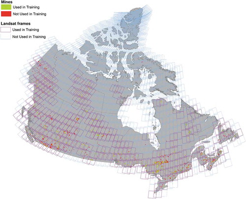
Figure 1. Indicates the number of Landsat-8 images required to cover the entire country of Canada for one time period. It also indicates the location of mines that were used in training and the locations of mines reserved for independent testing. In total, 1285 images are required to cover all of the training and testing mines for a single year.

Methods

For time-series consistency (i.e. trend consistency) in the APEI, when new methods are introduced into inventory, it is preferable to re-calculate the entire time-series using the new method. The Air Pollutant Inventory is reported as a time-series from 1990 and up to 2 years prior to the submission year. Therefore, in mine extent mapping for air pollutant emissions, ECCC must re-produce estimates of mine extents since 1990 using the new method. Specifically of interest are five “benchmark” years (1990, 2000, 2010, and the most recent year comprising a full growing season of data – 2018). We produced land-use classifications using a variety of remote sensing platforms for each of the benchmark years using the Random Forest classifier (Brieman, 2001). For 1990, 2000 and 2010, the Landsat-5 sensor (surface reflectance) was chosen for consistency between years. For 2018, a combination of Landsat-8 (surface reflectance), Sentinel-2 data (top of atmosphere), and Sentinel-1 (VV polarization) were tested with the intention of using one or a combination of these sensors for future estimates of mine extents. The use of different remote sensing platforms over the time-series may introduce some inconsistency between years, but the results are generally comparable as the spectral bands of the different optical sensors used here are similar. Sentinel-2 has a higher spatial resolution than Landsat-8 (15 m and 20 m vs 30 m), and therefore was expected to be the preferred sensor as it will result in a more detailed mine extent map. However, for the 2018 classification that included Sentinel-1 and Sentinel-2 data, we upscaled the Sentinel imagery to 30 m as Landsat imagery was also used. Sentinel-1 intensity information was thought to be useful for mapping waterbody extents (e.g. tailing ponds), and differentiating mines from the urban area due to sensitivity to differences in moisture and structure (Ulaby, Dubois, and van Zyl 1996; Dell’Acqua and Gamba 2003). In the optical imagery for each benchmark year, cloud and cloud shadow were masked, and a mosaic of “best available pixels” was created. To determine the best available pixel, first, the pixels that contain cloud and cloud shadow are excluded. Next, the remaining pixels are ranked based on pre-defined criteria. In this case, the pixel with the highest NDVI value was used as the “best” pixel. For each mosaic, only the growing-season data (June 15 – August 15) were used and based on the years immediately surrounding the benchmark year (e.g. 1989, 1990, 1991 for the 1990 benchmark year) because the single benchmark year often produced NoData in the mosaic due to persistent cloud in a single year. If more than one cloud-free pixel existed in the time series, the “greenest” pixel was selected to produce the mosaic of best available pixels (Li et al. 2019). Additionally, several indices were calculated (e.g. tasseled cap transformation (TCT; Crist and Cicone 1984), Normalized Difference Vegetation Index (NDVI; Tucker 1979), Soil Adjusted Vegetation Index (SAVI; Huete 1988), Soil Adjusted Total Vegetation Index (SATVI; Marsett et al. 2006), Modified Soil Adjusted Vegetation Index (MSAVI2; Qi et al. 1994), Band Ratio for Built Up Areas (BRBA; Zhou et al. 2014), and Normalized Built Up Area Index (NBAI; Zha, Gao, and Ni 2003)). Eighteen Grey-Level Covariance Matrix Texture parameters were also calculated (angular second movement, contrast, correlation, variance, inverse distance moment, sum average, sum variance, sum entropy, entropy, difference variance, difference entropy, information measure of corr. 1, information measure of corr. 2, max correlation coefficient, dissimilarity, inertia, cluster shade, cluster prominence; Haralick, Shanmugan, and Dinstein 1973). Digital Elevation Model (DEM) and slope values from Natural Resources Canada’s Canadian DEM were incorporated in GEE. All bands for each benchmark year were combined into a single Image Collection spanning the entire country.

Training and testing data were collected using a combination of ancillary data and image interpretation techniques. Initially, class development was iterative, starting with a binary classification (“mine vs non-mine”) and moving to more complex classifications in order to reduce confusion (errors of omission and commission) between important classes. For six classes, image interpretation was based on Landsat-5 for the year 2000 and a combination of Landsat-8, Sentinel-1 VV, and Sentinel-2 for the year 2018. For each year, single points were collected throughout the entire Canadian landmass in the following classes: permanent snow (n = 288), rock/outcrop (n = 696), vegetation (n = 5110), urban areas/roads/settlements (n = 820 in year 2000; n = 2066 in 2018), mines (n = 1079 in year 2000; n = 1740 in 2018) and permanent water (n = 2807). For permanent water, random points were created using the Global Surface Water dataset (Pekel et al. 2016), where the occurrence of permanent water was more than 90% certain. The number of training/testing data points within each class is not equal but roughly proportional to the expected proportions of each class (Millard and Richardson, 2015). For mines, several ancillary datasets were used to guide the interpreter in finding the general mine location, in order to collect quality training data. The publicly available CanVEC dataset “Mines, Energy and Communication Networks” (Natural Resources Canada 2017) indicated the general location of “ore” but locations were too approximate to use directly as training data (e.g. sometimes the location of the mine was at the mine office tens of kilometers from the actual mining operation). Centroids of mines digitized by Murray (1977) were manually extracted from the published maps of mine extents in 1977, under the assumption that these large mines would still be visible on the landscape (i.e. not fully recovered). And finally, data for non-active mines were extracted from Parsons et al. (2012). These three point datasets were combined and the interpreter used these data as a guide to create training/testing data throughout verified mine locations. Forty percent of all mine sites were reserved for independent “testing” based on a random selection (e.g. training and testing points were not collected at the same mine sites – Figure 2).

Random Forest Classification was performed within GEE, producing extents of mines for the entire landmass of Canada. Random Forest is a widely used machine learning classification algorithm and is known to produce high accuracy results, comparable to many other more complex algorithms (Fernandez-Delgado, Cernadas, and Barro 2014). Using an iterative approach, we performed initial testing experiments to determine the optimal combination of sensors and bands, optimal random Forest parameters and to determine if the training data collected would produce the desired level of accuracy. This means that we ran the Random Forest classier hundreds on times in GEE before deciding on an acceptable training dataset, predictor variables (bands, sensors) and model parameters. Through this process, it was determined that 250 trees within random forest produced acceptable accuracy and repeatability of results, and allowed the creation of the resulting extent maps in a reasonable time (i.e. more trees result in significantly longer processing times). Confusion matrices and the kappa statistic were calculated for the mine class based on independent testing data. Additionally, the pixel values of each training data point were extracted from GEE as a table for additional analysis in R (e.g. determining important variables is not available in the GEE JavaScript API). Although the initial training data points that were collected in the mining and urban classes produced good results for the year 2000, results were poorer in 2018 and therefore additional training data were collected in areas of new mines and new urban developments in 2018. In the case of urban areas/roads/settlements, all training data points that were collected for 2000 that were still present in subsequent years were therefore used as training or validation data. For mines, most training data points that were collected for the year 2000 were valid for other years; however, in some cases, flooding or re-vegetation of mines had occurred, and therefore each point needed to be visually inspected to determine if the class had changed. Any that did remain the same were re-used for training/validation in subsequent years.

In order to produce a classified result and map of mine extents from these images, training data were collected for two different time periods (Sentinel-1, Sentinel-2 and Landsat-8 data from 2018; Landsat-5 data from 2000). The training data created from 2018 image interpretation were used to build random forest models to classify both the Landsat-8 data and Sentinel-2 data for image collected between 2016–2018. Training data for the year 2000 was re-interpreted to capture changes in the landscape (e.g. new mines have opened, mines that existed in the past have been revegetated). The training data collected for the year 2000 image interpretation were used to train a random forest model based on the Landsat-5 data for the benchmark year 2000 (1999, 2000, and 2001), and additionally, the resulting random forest model was transferred to classify Landsat 5 data in the other two benchmark years (e.g. 1990 (1989, 1990, 1991) and 2010 (2009, 2010, 2011) (Figure 2)). While Random Forest does handle high dimensional data and is robust to redundant variables, it is common to perform a reduction of variables (i.e. variable selection) prior to running classifications in cases where a variable negatively impacts the results of classification. Therefore, we carried out an assessment of variable importance before running the classification that was used to map mine extents. Additionally, we performed an uncertainty assessment on our classification for the overall classification accuracy and mine classification accuracy by computing confidence intervals (α = 0.99), where a bootstrapped sample (without replacement) of 90% of the original training data was used in 100 model runs.

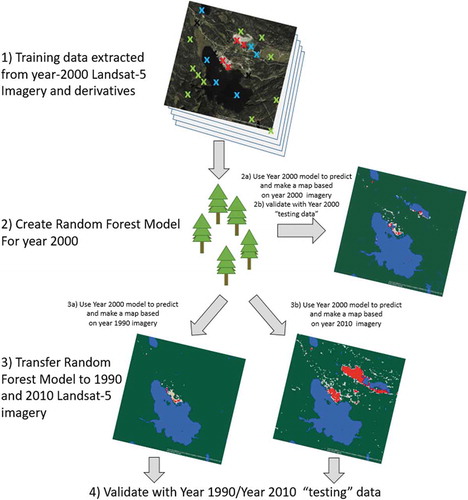
Figure 2. Training and testing data for the year 2000 were created using visual image interpretation of imagery from the year 2000. The spectral information at the location of each training data point was extracted for the year 2000 Landsat-5 imagery and indices/derivatives and then this data was used to build a random forest model to predict and map mines using the year 2000 mosaic. Because the Landsat-5 sensor was also used for two other benchmark years (1990 and 2010), this same model could then be “transferred” to the year 1990 and year 2010 mosaics to predict and map mines for those years. Each result was validated with independent data for the appropriate year.

Results

The results of all image classifications (i.e. Year 2018 Sentinel-1 & 2 + Landsat-8, Year 2000 Landsat-5 and transfer learning for Year 1990 and 2010) were very good, with independently validated overall accuracy higher than 90% in all cases (see Table 1–3). The results of the transfer learning between the Year 2000 and both the years 1990 and 2010 imagery indicated that models can be trained and then transferred to new dates for operational monitoring purposes.

Table 1. Model accuracy including overall classification accuracy, mine class accuracy, and kappa statistic for mine class.

Classification model	Mine class users' accuracy (%)	Mine class producer’s accuracy (%)	Mine class Kappa statistic	Overall classification accuracy (%)
Year 2000 Landsat-5 model transferred to Year 1990 imagery	83.3	85	0.49	91.2
Year 2000 Landsat-5 model classifying Year 2000 imagery	90.6	83.8	0.65	92.5
Year 2000 Landsat-5 model transferred to year 2010 imagery	80.6	81.4	0.47	94.8
Year 2018 Landsat-8, Sentinel-1, Sentinel-2 model	88.7	88.5	0.60	91.8

For the mine class, User’s and Producer’s accuracies were all better than 80% with the Year 2000 Landsat-5 classification producing the highest User’s accuracy (90.6%) and the Year 2018 classification (combining Landsat-8, Sentinel 1&2) with the highest Producer’s accuracy (Table 1). Consistently, any misclassifications in the mine class were within urban areas, and occasionally within snow or water classes (See Table A1.–4). The results of the rock and permanent snow class were highly variable between the different classifications with accuracies ranging from 34% to 100%. However, it is important to note that these classes contained significantly fewer training data points than the other classes due to their much smaller area in the landscape and difficulty in determining high-quality training data through visual interpretation. Based on the uncertainty assessment (Tables 2 & 3), the model runs were very consistent and overall the error was low. Therefore, the confidence intervals are quite small and the range of values is not significantly different from the model run with all data points. Some of the differences between model runs can be attributed to the random nature of the randomForest algorithm (e.g. random subset of variables used to test the split, and random subset of data points used to train the model).

Table 2. Uncertainty assessment of overall classification: confidence intervals (CI) were computed based on 100 runs of the random forest algorithm with a bootstrapped sample of data (90%).

Year – overall	Error %	Upper CI % accuracy	Lower CI % accuracy
1990	0.11	92.75	91.53
2000	0.17	92.70	92.36
2010	0.09	91.46	91.28
2018	0.06	91.24	91.13

Table 3. Uncertainty assessment of mine class: confidence intervals (CI) were computed based on 100 runs of the random forest algorithm with a bootstrapped sample of data (90%).

Year – mine class	Error %	Upper CI %	Lower CI %
1990	0.12	83.84	83.60
2000	0.19	90.98	90.60
2010	0.30	81.68	81.08
2018	0.07	88.52	88.38

Table A1. Confusion matrix for the Year 2000 Landsat-5 model transferred to the Year 1990 imagery (independent validation with the Year 1990 testing data).

	Mines	Water	Urban	Vegetation	Rock	Snow	User’s accuracy (%)
Mines	549	41	53	8	0	8	83.3
Water	26	900	8	31	1	0	93.2
Urban	25	2	78	25	0	0	60.0
Vegetation	1	7	4	1004	0	0	98.8
Rock	2	3	0	1	67	2	89.3
Snow	43	5	0	0	1	48	49.5
Producer’s accuracy (%)	85.0	94.0	54.6	93.9	97.1	82.8	Overall: 92.1%

Figures 3–5 all indicate that mine area increased steadily between 1990 and the present day. The large increase in area of mines between 1977 and 1990 is likely due to an underestimation in the areas calculated by Murray et al. (1977), as this study was not meant to be an exhaustive mapping exercise, but focused on the largest mines and only mines with a minimum mapping unit greater than 10 ha. For 1990 onwards, out results were exhaustive, “wall to wall” mapping of mines across Canada and our minimum mapping unit is technically one 30-m pixel (i.e. 0.1 ha), although it is likely that mines that small are visually indistinguishable from noise in the results.

Figure 3. Graph indicating the total change in the area of exposed mine waste extent since 1977. The area of mines in 1977 is estimated from Murray et al. (1977) and the area of mines in 1990–present day is estimated using mapped results in GEE.

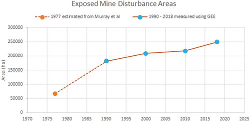
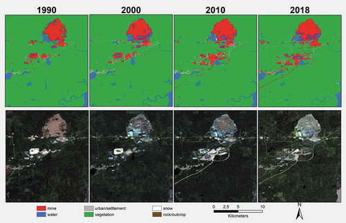
Figure 4. Example A map showing mine change over time and corresponding imagery. It is clear that the area of “rock/outcrop” increases over time and between the annual classifications.

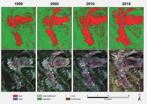
Figure 5. Example B map showing mine change over time and corresponding imagery. Significant areas of mine expansion and changes in the distribution of settling ponds are visible in the center of the image.

Discussion

Previous estimates of particulate matter for the Canadian Air Pollutant Emissions Inventory (APEI) were based on the exposed mine disturbance areas that had been calculated using out-dated mine area extents. The recent availability of Big Geospatial Data tools and analysis techniques in remote sensing (such as Google Earth Engine) enables scientists to produce more precise estimates of particulate matter, leading to more precise predictions of air quality and increasing the reliability of the air quality warning system in Canada and internationally. Due to resource limitations, the use of nation-wide, time-series remote sensing was not possible for the APEI in past years. Accessing the entire Landsat archive in the cloud enabled significant improvement to the methods for future APEI reports. We estimate that the data required to complete this study represent more than 10 TB of drive space for raw data alone.

Although GEE provides a powerful platform for large area and long-time series analysis, our results are not without error. As in all cases where a supervised classifier is used to produce land-cover/land-use maps, the quality of the results are dependent on the quality of the training data provided to the classifier (Millard and Richardson, 2015). While the overall accuracy of all the classifications was very high, these results are somewhat skewed as the vegetation and water classes were well classified and represented the largest sample of training/testing data. We have chosen not to reduce the number of data points in the water and vegetation classes because (1) Mine class accuracy was within the level that was acceptable to our application and (2) we could not capture the full distribution of spectral and radar signatures with a significantly smaller sample. Doing so resulted in errors of omission, that were identified visually. As no reliable, current-day extents of mines were available, a combination of expert image interpretation combined with ancillary data provided the best available information about mines and other classes. Although this method resulted in high accuracy in the mine class as well as most other classes, we cannot assess errors on omission on behalf of the interpreter. For example, there may be types of mines that were not easily visually distinguished from other classes (e.g. gravel pits from areas of rock).

Confusion between mines and other classes

Initially, all classes were well classified with the exception of “outcrops/rock.” The addition of the elevation and slope variables improved the misclassification of mines as outcrop/rocks in mountainous areas (e.g. British Columbia) but there were still many rock areas being misclassified as mines in Taiga Shield ecozone where extensive areas of granite outcrop exist. We experimented with removing the outcrop/rock class from training/testing data collection, but this resulted in many errors of commission with mine class in these cases.

Visual analysis of the classification results indicated some errors of commission in urban areas (e.g. parking lots/industrial areas) that may not have been captured by the independent validation data due to the relatively small number of training and validation data created for this large study area. For our operational purposes, these areas will be masked out using ancillary datasets (e.g. footprints of urban developments); however, ideally, the collection of a larger training data sample should be collected to capture the variability in these two classes. In our initial trials, there was significant confusion between mines and urban areas, but the addition of Sentinel-1 VV (radar) leads to some improvements. Despite the increase in accuracy, within the exposed mine disturbance areas, several pixels were also visually identified that were classified as urban. These were usually paved roads and buildings within the mining areas. Initially, we assumed these were misclassifications that were not being assessed by our testing set (as the expert interpreter did not collect training or testing pixels on buildings within the area of a mine). However, based on our specific application, buildings and paved roads at mine sites do not contribute to particulate matter in the same way that exposed waste rock and tailings do. Therefore, these were determined to be correctly classified. This issue highlights a shortcoming of using a relatively small number of training data points (approximately 11 000) to classify a very large area (the entire landmass of Canada) with great variability within the classes. Although the interpreter attempted to collect training data points that were representative of all of the mine types as well as the variability in the other classes, more training data may be required to better distinguish classes as similar as outcrops/rock, mines, and urban areas. This problem is not specific to our application but to any large-scale mapping application but is an important issue for anyone using GEE.

Remote sensing predictors

As a mosaic of the “best available pixel” was created within the growing seasons of 3 years for any given “benchmark year,” the results of the mosaic are not always easily interpretable. For example, as Landsat-8 has a 16-day repeat-time and our growing-season window represented 45 days, each pixel within a single Landsat image footprint could actually represent the value of one of the four different dates. Thinking of the mosaic of the extent of the Canadian landmass rather than of a single image, the specific acquisition dates of a Landsat image will vary based on their unique location and therefore any pixel within the mosaic may actually represent the spectral reflectance on a date within our window. We aimed to minimize the width of the date range to increase the similarity in pixels throughout the mosaic, but also allow enough images to be included in the calculation of “best available pixel” so that a cloud-free image would be found for every pixel. In the future, results could be improved by using a sliding-date range based on the variability of growing season throughout the study area.

Due to a large number of image inputs used to create the random forest models and the large extent of the area being classified, the creation and export of the predicted map from GEE required the largest portion of time in the classification process. Therefore, we attempted to reduce the number of variables included in the model. The random forest classification algorithm computes Mean Decrease in Accuracy (MDA) which is commonly used to assess variable importance. No functions exist within GEE (yet) to analyze the importance of variables in a random forest classifier therefore this was completed using extracted training data values in R. It was found that elevation, Sentinel-2 Blue, Sentinel-2 Modified Soil Adjusted Vegetation Index, and Landsat-8 Normalized Difference Water Index were most important channels for the mine class and other channels contributed significantly less. These “important” channels indicate that mines can be differentiated from other classes based on elevation, soil and vegetation characteristics. For the overall classification, elevation, Landsat-8 TIRS1 and TIRS2, Sentinel-1 VV and Tasseled Cap Wetness were the most important channels in classification. In both cases, elevation appeared to be the most important channel; however, we suspect this is because it is the only channel that can separate mines from bare rock, where most of the bare rock areas exist at high elevations in the Rocky Mountains. The GLCM texture variables were found to be negatively impacting the classification (MDA < 0) and were therefore removed. However, the spatial patterns of entropy and contrast visually appeared to distinguish mine areas from many other classes but the pixel values themselves were not homogeneous within the mine class and therefore they were poor predictor variables in a pixel-based classifier. These variables may be well suited for an object-oriented classification and therefore future work will investigate the application of OBIA in GEE.

Transferring models across time

One significant advantage of GEE was the ability to access all data in the Landsat archive and build models that could be transferred across time. The Landsat-5 archive spans 1984 to 2013, thereby producing a consistent coverage in time with the same sensor parameters (e.g. the same wavelengths per band for any given image). This allowed us to build a model using training data collected in only the Year 2000 but transfer that model to other years to produce predictions without collecting training data for that new year. We did, however, collect a smaller subset of validation data for these years in order to validate the applicability of the transfer between years. The kappa statistic calculated for the mine class indicated that the models that were transferred were less reliable than the models built with training data from the same year but still within the range that was appropriate for our application. In the future, we plan to use the 2018 model built with Landsat-8, Sentinel-2, and Sentinel-1 (VV) to monitor changes in mine extents in the future using transfer learning as we did here with Landsat-5.

Moving from classification to estimating emissions

While the exposed mine-waste area is required to estimate air quality emissions from mines, in fact, it is the area of fine tailings, not the total surface area that is used to estimate emissions. Historically, the ratio of fine tailings has been estimated as one third of the total mine waste exposure area and this ratio has been implemented again in the 2019 inventory. Therefore, further work is required to differentiate types of mine waste, as well as the size of mine waste materials, as the particle size is important in estimating the material’s aerial distribution. In this case, higher spatial resolution imagery or hyperspectral imagery might be required to differentiate waste rock from tailings piles. Tailings piles of fine silt size are more likely to produce particulate matter than waste rock but these two waste materials are often spectrally similar as they can contain much of the same materials.

While an official “methods change” to the APEI has been accepted to include the new methods describe here, other changes have also been made to estimate mine waste emissions in the 2020 APEI, including a change to the weather correction factor, and a correction to a miscalculation in tabulation that has been carried through erroneous code. Therefore, while the newly calculated area of exposed mine waste has increased, a comparison of the emissions estimates generated using the newly derived areas with the previously published estimates indicates more than 90% reduction in absolute emissions. Specifically, in 2010 the estimated area of exposed mine waste calculated using remote sensing was one third larger in comparison with previous estimates of areas that had been used in the APEI. Conversely, 33,000 tonnes was the previously published estimate of TM for 2010, but based on the new method changes, only 2000 tonnes TM was emitted.

In the future, ECCC has plans to expand the use of the Google Earth Engine for mapping other pollutants and emissions. For example, any land-use changes result in either an emission (source) or removal (sink) of carbon which needs to be accounted for in the National Inventory Report of Greenhouse Gas Emissions and in many cases these changes in land-use need to be mapped for the same benchmark years as noted above. Future work will also assess the ability to look at temporal signatures to detect changes in land-use rather than performing change analysis based on classifications at two different times-periods.

Conclusions

The calculation of the area of exposed mine waste across the Canadian land-mass has allowed Environment and Climate Change Canada (ECCC) to refine their estimates of air pollutant emissions for the Air Pollutant Emissions Inventory and provide better information to the public about air quality risks to health. Overall, Google Earth Engine (GEE) proved to be an invaluable tool for ECCC in mapping exposed mine waste areas and would be similarly useful for any organization with large-area monitoring mandates or those interested in time-series analysis of the Landsat archive. This tool has enabled the monitoring of mine growth over a 30-year period and has confirmed that overall the area of mines is growing in Canada. The ability to process this large amount of data in the cloud using only a web-browser has enabled ECCC to produce highly accurate estimates of mine extents and improve estimates of air quality emissions. Almost 12 000 training data points were collected throughout Canada for both the years 2000 and 2018. Transfer learning was used to build predictive classifications for the years 2010 and 1990 as well. In all cases, models resulted in greater than 90% overall accuracy overall and greater than 80% accuracy in the mine class. Quality training data that captured the full variability in the different classes were key to obtaining high-quality mapping results.

Acknowledgements

The authors would like to thank the anonymous reviewers for taking the time to read and improve their manuscript. We would like to thank Kristen Obeda (ECCC) for her contribution to the extracting area and centroid information from the Murray et al. (1977) report. Dominique Blain (ECCC) is thanked for reading and providing comments on early versions of the manuscript.

Disclosure statement

No potential conflict of interest was reported by the authors.

Additional information

Funding

This work was supported by funding from Environment and Climate Change Canada..

Appendix

Table A2. Confusion matrix for the Year 2000 Landsat-5 model classifying the Year 2000 imagery (independent validation with the Year 2000 testing data).

	Mines	Water	Urban	Vegetation	Rock	Snow	User’s accuracy (%)
Mines	310	14	13	3	0	2	90.6
Water	13	900	0	26	4	0	95.4
Urban	22	3	127	1	0	0	83.0
Vegetation	5	10	2	985	1	0	98.9
Rock	4	28	0	26	51	0	46.8
Snow	16	0	1	0	0	41	70.7
Producer’s accuracy (%)	83.8	94.2	88.8	94.7	91.1	95.4	92.5%

Table A3. Confusion matrix for the Year 2000 Landsat-5 model transferred to the Year 2010 imagery (independent validation from the Year 2010).

	Mines	Water	Urban	Vegetation	Rock	Snow	User’s accuracy (%)
Mines	258	21	38	1	0	2	80.6
Water	17	920	6	24	0	0	95.1
Urban	23	1	97	9	0	0	74.6
Vegetation	5	10	4	1712	0	1	98.9
Rock	0	0	0	0	30	0	100.0
Snow	14	2	0	0	1	16	48.5
Producer’s accuracy (%)	81.4	96.4	66.9	98.1	96.8	84.2	Overall = 94.8%

Table A4. Confusion matrix for Year 2018 Landsat-8, Sentinel-1, and Sentinel-2 model (independent validation).

	Mines	Water	Urban	Vegetation	Rock	Snow	User’s accuracy(%)
Mines	391	6	36	3	0	5	88.7
Water	7	499	2	3	0	1	97.5
Urban	36	0	334	3	0	0	89.5
Vegetation	0	3	0	596	0	0	99.5
Rock	3	11	0	15	20	10	33.9
Snow	5	7	0	21	0	146	81.6
Producer’s accuracy (%)	88.5	94.9	89.8	93.0	100.0	90.1	Overall: 91.8%

References

- Breiman, L. 2001. “Random Forests.” Machine Learning 45: 5–32.
- Canada, N. R. (2017). “Mines, Energy and Communication Networks in Canada - CanVec Series.” [Data file]. https://open.canada.ca/data/en/dataset/92dbea79-f644-4a62-b25e-8eb993ca0264
- Chen, B., X. Xiao, X. Li, L. Pan, R. Doughty, J. Ma, J. Dong, et al. 2017. ““A Mangrove Forest Map of China in 215: Analysis of Time Series Landsat 7/8 and Sentinel −1A Imagery in Google Earth Engine Cloud Computing Platform.” ISPRS Journal of Photogrammetry and Remote Sensing 131: 104–120. doi:10.1016/j.isprsjprs.2017.07.011.
- Chopin, E. I. B., and B. J. Alloway. 2007. “Trace Element Partitioning and Soil Particle Characterisation around Mining and Smelting Areas at Tharsis, Riotinto and Huelva, SW Spain.” Science of the Total Environment 373: 488–500. doi:10.1016/j.scitotenv.2006.11.037.
- Corriveau, M., H. Jamieson, M. Parson, J. Campbell, and A. Lanzirotti. 2011. “Direct Characterization of Airborne Particles Associated with Arsenic-rich Mine Tailings: Particle Size, Mineralogy and Texture.” Applied Chemistry 26: 1639–1648.
- Crist, E., and R. Cicone. 1984. “A Physically-Based Transformation of Thematic Mapper Data—The TM Tasseled Cap.” IEEE Transactions on Geoscience and Remote Sensing GE-22 (3). doi:10.1109/TGRS.1984.350619.
- Dell’Acqua, F., and P. Gamba. 2003. “Texture-based Characterization of Urban Environments on Satellite SAR Images.” IEEE Transactions in Geoscience and Remote Sensing 41 (1): 153–159. doi:10.1109/TGRS.2002.807754.
- Ekosse, G., D. J. van den Heever, L. de Lager, and O. Totolo. 2004. “Environmental Chemistry and Mineralogy of Particulate Air Matter around Selebi Phikwe Nickel–Copper Plant, Botswana.” Mineral Engineering 53 (17): 349. doi:10.1016/j.mineng.2003.08.016.
- Environment and Climate Change Canada (ECCC). (2013a). “Online.” Accessed 31 August 2019. https://www.canada.ca/en/environment-climate-change/services/air-pollution/pollutants/common-contaminants/particulate-matter.html
- Environment and Climate Change Canada (ECCC). (2013b). “Online.” Accessed 31 August 2019. http://www.ec.gc.ca/default.asp?lang=En&n=56D4043B-1&news=A4B2C28A-2DFB-4BF4-8777-ADF29B4360BD
- Environment and Climate Change Canada (ECCC). (2019). Online. Accessed 31 August 2019. https://www.canada.ca/en/environment-climate-change/services/air-quality-health-index.html
- Evans, J., and D., . Cooper. 1980. “An Inventory of Particulate Emissions from Open Sources.” Journal of the Air Pollution Control Association 30 (12): 1298–1303. doi:10.1080/00022470.1980.10465188.
- Fernandez-Delgado, M., E. Cernadas, and S. Barro. 2014. “Do We Really Need Hundreds of Classifiers to Solve Real World Classification Problems?” Journal of Machine Learning Research 15: 3133–3181.
- Gorelick, N., M. Hancher, M. Dixon, D. Thau, and R. Moore. 2017. “Google Earth Engine: Planetary-scale Geospatial Analysis for Everyone.” Remote Sensing of Environment 202: 18–27.
- Haralick, R., K. Shanmugan, and I. Dinstein. 1973. “Textural Features for Image classification”.” IEEE Transactions on Systems Man, and Cybernetics SMC-3 (6): 610–621. doi:10.1109/TSMC.1973.4309314.
- Hinds, W. C. 1999. Aerosol Technology: Properties, Behavior, and Measurement of Airborne Particles. 2nd ed. New York: Wiley-interscience.
- Huete, A. 1988. “Soil Adjusted Vegetation Index (SAVI).” Remote Sensing of Environment 25 (3): 295–309. doi:10.1016/0034-4257(88)90106-X.
- Informetrica. 2002. Infometrica Economic Index Database “1981–2024.”
- IPCC. (2006). “Revised 1996 IPCC Guidelines for National Greenhouse Gas Inventories: Reference Manual, Chapter 5.” Online, Accessed 6 Nov 2019. https://www.ipcc-nggip.iges.or.jp/public/gl/guidelin/ch5ref1.pdf
- Johansen, K., S. Phinn, and M. Taylor. 2015. “Mapping Woody Vegetation Clearing in Queensland, Australia from Landsat Imagery Using Google Earth Engine.” Remote Sensing Applications: Society and Environment 1: 36–49. doi:10.1016/j.rsase.2015.06.002.
- Li, H., W. Wan, Y. Fang, S. Zhu, X. Chen, B. Liu, and Y. Hong. 2019. “A Google Earth Engine-enabled Software for Efficiently Generating High-quality User-read Landsat Mosaic images”.” Environmental Modelling and Software 112: 16–22. doi:10.1016/j.envsoft.2018.11.004.
- López, M., I. González, and A. Romero. 2008. “Trace Elements Contamination of Agricultural Soils Affected by Sulphide Exploitation (Iberian Pyrite Belt, SW Spain).” Environmental Geology 54: 805–818. doi:10.1007/s00254-007-0864-x.
- Marsett, R. C., J. Qi, P. Heilman, S. H. Biedenbender, M. C. Watson, S. Amer, M. Weltz, D. Goodrich, and R. Marsett. 2006. “Remote Sensing for Grassland Management in the Arid Southwest.” Rangeland Ecology and Management 59: 530–540. doi:10.2111/05-201R.1.
- Millard, K., and M. Richardson. 2015. “On the importance of training data sample selection in random forest image classification: A case study in peatland ecosystem mapping.” Remote Sensing 7: 8489–8515.
- Murray, D. 1977. CANMET Report. Pit-slope manual, Mine Waste Inventory by Satellite imagery. 77 (58). University of California Press.
- Parsons, M.B., K.W.G. LeBlanc, G.E.M. Hall, A.L. Sangster, J.E. Vaive, and P. Pelchat (2012). Environmental Geochemistry of Tailings, Sediments and Surface Waters Collected from 14 Historial Gold Mining Districts in Nova Scotia. Geological Survey of Canada Open File 7150. doi:10.4095/291923
- Patel, N., E. Angiuli, P. Gamba, A. Gaughan, G. Lisini, F. Stevens, A. Tatem, and G. Trianni. 2015. “Multitemporal Settlement and Population Mapping from Landsat Using Google Earth Engine.” International Journal of Applied Earth Observation and Geoinformation 35B: 199–208.
- Pekel, J., A. Cottam, N. Gorelick, and A. Belward. 2016. “High-resolution Mapping of Global Surface Water and Its Long-term Changes.” Nature 540: 418–422. doi:10.1038/nature20584.
- Pericak, A., C. Thomas, D. Kroodsma, M. Wasson, M. Ross, N. Clinton, D. Campagna, Y. Franklin, D. Bernhardt, and J. Amos. 2018. “Mapping the Yearly Extent of Surface Coal Mining in Central Appalachia Using Landsat and Google Earth Engine.” Plos One. doi:10.1371/journal.pone.0197758.
- Pumlee, G. S., and S. A. Morman. 2011. Mine Wastes and Human Health. Elements, 7(6): 399–404. doi:10.2113/gselements.7.6.399
- Qi, J., A. Chehbouni, A. Heuete, Y. Kerr, and S. Sorooshian. 1994. “A Modified Soil Adjusted Vegetation Index.” Remote Sensing of Environment 48: 119–126. doi:10.1016/0034-4257(94)90134-1.
- Townsend, P., D. Helmers, C. Kingdon, B. McNeil, M. de Beurs, and K. Eshleman. 2009. “Changes in the Extent of Surface Mining and Reclamation in the Central Appalachians Detected Using 1976-2006 Landsat Time Series.” Remote Sensing of Environment 1 (15): 62–72. doi:10.1016/j.rse.2008.08.012.
- Tucker, C. J. 1979. “Red and Photographic Infrared Linear Combinations for Monitoring Vegetation.” Remote Sensing of Environment 8 (2): 127–150. doi:10.1016/0034-4257(79)90013-0.
- Ulaby, F., P. Dubois, and J. van Zyl. 1996. “Radar Mapping of Surface Soil Moisture.” Journal of Hydrology 184 (1–2): 57–84. doi:10.1016/0022-1694(95)02968-0.
- Zha, Y., J. Gao, and S. Ni. 2003. “Use of Normalized Difference Built-Up Index in Automatically Mapping Urban Areas from TM Imagery.” International Journal of Remote Sensing 24 (3): 583–594. doi:10.1080/01431160304987.
- Zhang, H., Q. Li, J. Liu, J. Shang, X. Du, L. Zhoa, N. Wang, and T. Dong. 2017. “Crop Classification and Acreage Estimation in North Korea Using Phenology Features.” GIScience and Remote Sensing 54: 381–406.
- Zhou, Y., G. Yang, S. Wang, L. Wang, F. Wang, and X. Liu. 2014. “A New Index for Mapping Built-up and Bare Land Areas from Landsat-8 OLI Data.” Remote Sensing Letters 5 (10): 862–871. doi:10.1080/2150704X.2014.973996.