Use of Local Climate Zones to investigate surface urban heat islands in Texas

ABSTRACT

Urban heat islands (UHIs) are a key topic in urban climate studies. However, systematic criteria for UHI comparisons were lacking prior to 2012, when the concept of Local Climate Zones (LCZs) was introduced. By relating remotely sensed land surface temperature (LST) to LCZs, we explored the applicability of LCZs in surface urban heat island (SUHI) investigations and compared the LST variation within and among LCZs for the Austin, San Antonio, and Dallas-Fort Worth metropolitan areas in Texas, United States. Landsat 8 images from one summer and one winter day in 2015 were used to obtain LSTs to measure and model SUHIs. LCZs that were characterized by different land covers had the greatest LST variations, and LCZs that were further characterized by various urban morphological properties (including building density and height of roughness) also showed significant LST differences. Moreover, LCZ 9 (sparsely built), LCZ 10 (heavy industry), LCZ D (low plants), LCZ E (bare rock or paved), and LCZ F (bare soil or sand) tended to contribute to contradictory heating/cooling effects in different metropolitan areas, primarily due to the spatial arrangement and geographic locations of LCZs. The close association between LCZs and LST demonstrates that LCZs are valuable for comparative analysis of the SUHI phenomenon between different cities and can be helpful for examination of the evolution of SUHIs over time. Our findings further suggest that understanding the spatial distribution of LCZs can benefit the development of mitigation strategies for SUHIs.

KEYWORDS:

• Land surface temperature
• Landsat
• Local Climate Zones
• surface urban heat island
• Texas cities

1. Introduction

Although urban land area accounts for only a small fraction (nearly 3%) of the Earth’s terrestrial surface (Lambin et al. 2001; Liu et al. 2014), they are host to more than 70% of all human economic activities (Schneider, Friedl, and Potere 2010). Urban densification and expansion increases built-up areas, altering the natural surface energy and water balances and often results in increased urban flooding, air pollution, heat islands, etc. In the urban canopy layer (UCL, i.e., the volume of air extending from ground level to the height of rooftops and urban treetops (Oke 1976)), these underlying characteristics lead to an increase of short-wave radiation absorption, long-wave radiation and sensible heat storage, decreased evapotranspiration and total turbulent heat transport, and increases in sensible heat input-entrainment within the urban boundary layer (UBL) (Landsberg 1981; Oke and Cleugh 1987). Consequently, urban areas exhibit higher air and surface temperatures compared to the surrounding countryside, a phenomenon known as the urban heat island (UHI) effect.

For UHI studies, the air temperature being investigated is generally divided into two broad categories according to the causal processes and measurement methods: UCL UHI (Oke 1995) at the microscale and UBL UHI at the mesoscale (Barlow 2014). The UCL UHI is usually measured in-situ, while special platforms (e.g., radiosondes, aircraft) are used to collect UBL UHI measurements. Discrete categorization of the metropolitan landscape adds uncertainty to measurements of UCL UHI because the “point measurement” of air temperature is inadequate to thoroughly describe its spatial heterogeneity. As such, the limited monitoring stations associated with UCL or UBL UHI measurements are usually insufficient to capture the heterogeneous thermal characteristics for urban landscape planning or urban climate studies (Hu and Brunsell 2015; Shen et al. 2016). A Surface Urban Heat Island (SUHI) is observed using land surface temperature (LST), where values are time-synchronized and spatially continuous with pixel values over a large extent.

Compared to traditional air temperature measurements, remote sensing measurement of surface temperatures and associated analytical techniques facilitate a deeper understanding of spatial thermal patterns (Weng, Lu, and Schubring 2004) and the influence of surface properties on SUHI formation (Buyantuyev and Wu 2009; Zhao et al. 2018). Nonetheless, some uncertainties associated with applying satellite imagery to study the SUHI phenomenon are still present including the underlying methodological constraints, limited revisit intervals, and consistent acquisition times for days under investigation. Additionally, because of their nadir-looking position, passive multispectral sensors provide only a plan view of the surface (2-D temperatures) and thereby exclude vertical (3-D) temperatures and “hidden” surfaces (e.g., building walls, shaded ground beneath trees). In terms of spatial variation of LST, several studies have incorporated the criteria of built-up land intensity and configuration (Zhou et al. 2014), or Impervious Surface Area (ISA) (Imhoff et al. 2010). For instance, ISA was used to investigate the SUHI amplitude and its relationship to development intensity, size, and ecological setting for 38 metropolitan areas in the continental United States (Imhoff et al. 2010). However, these criteria were based on a single characteristic (e.g., ISA) and related to surface temperature and local climate.

To standardize observation protocols, the Local Climate Zones (LCZs) concept was introduced in 2012 to improve the documentation and analysis of UHI observations (Stewart and Oke 2012). LCZs are defined as “regions of uniform land cover, surface structure, construction material, and human activity that span hundreds of meters to several kilometers on a horizontal scale” (Stewart and Oke 2012, 1884). The 17 standard LCZ classes (see Table A1) are determined by their surface characteristics, including: cover (permeability), structure (building and tree height and spacing), fabric (albedo, thermal admittance), and metabolism (anthropogenic heat flux). Unique combinations of these properties provide a distinct thermal regime for each LCZ (Geletič, Lehnert, and Dobrovolný 2016; Stewart, Oke, and Krayenhoff 2014).

Although the LCZ concept was initially designed for atmospheric UHI studies, ongoing research has explored the applicability of LCZs for SUHI investigation. Compared to traditional SUHI investigation, LCZ-related mapping methods provide a standardized measure for understanding SUHI because they are grounded in the zoning practices enacted on urban spaces. With this universally accepted standard, it became possible to make a comprehensive, comparative analysis of SUHI. For instance, Geletič, Lehnert, and Dobrovolný (2016) indicated, by using cases in Europe, that LCZ classes are distinguishable from each other in terms of surface temperature. An LCZs mapping study of the Yangtze River Delta megapolitan region in China further showed LST variation among LCZs (Cai, Ren, and Xu 2017). Kotharkar and Bagade (2018) assessed the inter-LCZ air temperature difference and identified LCZs at Nagpur city with stationary meteorological observation and mobile surveys.

However, due to the heterogeneity of urban landscapes and the general lack of building structure information, there are considerable challenges for creating reliable LCZ maps worldwide. For example, WUDAPT (e.g., World Urban Database and Access Portal Tools) has conducted dozens of studies with free software and data (Xu et al. 2017), but appropriate quantitative assessments still need to be provided (Verdonck et al. 2017).

Within the last several years, a growing body of literature has emerged that evaluates the potential and suitability of the LCZ concept for UHI applications (e.g., Richard et al. 2018) and for studying LST variation and the SUHI phenomenon. LST variation among LCZs have also been studied and explored in cities and areas worldwide, including North America (Wang et al. 2018), western (Nassar, Blackburn, and Whyatt 2016) and eastern Asia (Cai, Ren, and Xu 2017; Cai et al. 2018; Khamchiangta and Dhakal 2019; Simanjuntak, Kuffer, and Reckien 2019; Wang, Zhan, and Ouyang 2017), Australia (Koc et al. 2018), Europe (Richard et al. 2018), and Africa (Mushore et al. 2019; Richard et al. 2018). Although GIS-based LCZs mapping can efficiently utilize local administrative data, the comparison of LCZs maps as well as comparisons of SUHI phenomenon across multiple metropolitan areas worldwide remains challenging (Hidalgo et al. 2019).

An investigation of the thermal behavioral characteristics of individual LCZs is clearly warranted for SUHI comparison and assessment of intra-urban distributions. In this study, we compare SUHI effects for the Dallas-Fort Worth, Austin, and San Antonio metropolitan areas in Texas, USA. Specifically, we attempt to link a series of Landsat-derived LSTs with LCZ categories to: 1) examine the applicability and effectiveness of analyzing LST variations with LCZ maps; and 2) investigate how LCZs affect the SUHI phenomenon by facilitating comparative analysis of the three case study areas.

2. Study areas and their Local Climate Zones

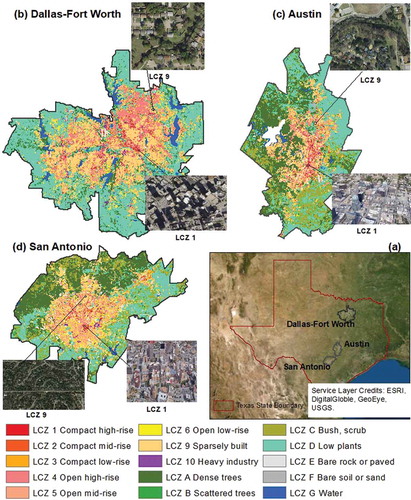
Our study areas are located in the northeastern (Dallas-Fort Worth) and central (Austin and San Antonio) regions of Texas, USA (Figure 1(a)) and are among the largest population and economic centers in Texas. Despite similarities among the urban regions in these metropolitan areas (e.g., socioeconomic development, topography, etc.), each area has unique characteristics in terms of climatic features and ecological environments (Table 1).

Table 1. General climatic and population features of the studied cities

	Dallas-Fort Worth	Austin	San Antonio
Average daily mean air temperature (°C)
January	9	11	11
July	31	30	30
Average precipitation (mm)	324.6	255.4	316.4
Elevation (min/max, Average) (m)	(106/271, 163) (Dallas) (136/367, 218) (Fort-Worth)	(116/440, 229)	(125/609, 261)
Ecological regions	Oaks and Prairies Osage Plains (Cross Timbers)	Edwards Plateau Oaks and Prairies	Oaks and Prairies Edwards Plateau South Texas Brushlands
Estimated population (2015)	1,260,688 (Dallas) 796,614 (Fort-Worth)	887,061	1,413,881

Notes: Average air temperature and precipitation data are based on Time and Date AS (https://www.timeanddate.com). Elevation data are acquired from Topographic Maps (https://en-gb.topographic-map.com). The type of biome of the ecological region is defined according to the Texas Parks and Wildlife Department (TPWD) Ecological Mapping System. Population statistics are based on the American Community Survey by the U.S. Census Bureau (2015).

Figure 1. Study area boundaries (a) and the Local Climate Zone (LCZ) distributions (b, c, d) with examples of the typical LCZs from Google Earth

The extremely fast growth of these three metropolitan areas has attracted attention from urban designers to work to prevent low-density urban sprawl. Planners have adopted and implemented environmental regulations stemming from detailed initiatives and ordinances for managing built-up and greenspaces throughout their respective cities (Austin City Council 2012; City of Austin Neighborhood Planning and Zoning Department 2008; Dallas City Council 2006; San Antonio City Council 2016). A recent investigation of the City of Austin has revealed positive indicators of sustainable urban design initiatives on “compact and connected” development since the mid-2000s (Zhao, Weng, and Hersperger 2020). However, environmental issues such as the heating effect associated with urban landscape forms needs to be further studied to promote the integration of urban planning and design into strategic heat mitigation. There has been limited scientific research and insufficient analysis of SUHI for our study areas (Darby and Senff 2007; Xie, et al. 2005; Boice, et al. 2018). In a recent study of Austin, Texas, Kim et al. (2016) found that larger green space patches in close proximity resulted in lower LST at the neighborhood level. Although this information is useful and informative, a more thorough characterization and understanding of the urban morphology and SUHI effect is needed for Texas cities.

Following the definition of LCZs by Stewart and Oke (2012), Zhao et al. (2019) mapped the LCZs of our study areas using a combination of lidar and sub-orbital image data. Variables related to land cover, the height of roughness features, building composition and configuration, permeable surface proportion, and city land use planning codes and datasets were analyzed and ultimately classified as LCZ mapping variables (Zhao et al. 2019) (Figure 2). Considering that building structure affects local climate, the ranges of variograms for building heights were calculated and 270 m was chosen for the LCZs mapping unit. As part of the LCZ mapping scheme, the accuracy of the LCZ mapping was tested in terms of sky view factor, aspect ratio, and terrain roughness using thresholds defined by Stewart and Oke (2012). Google Earth was used to demonstrate the reliability of the LCZ maps by overlaying LCZs with historical imagery. Table A1 in the appendix provides the spatial characteristics of individual LCZ patch size and overall LCZs pattern diversity for the three study areas. Most of our LCZs were matched correspondingly with the representative examples shown in Table 2 in p. 1885 of (Stewart and Oke 2012). The LCZs maps capture most of the underlying land cover and urban morphological characteristics, with <1% of the total area not assigned to an LCZ category. LCZs (Zhao et al. 2019).

Table 2. Ambient environmental conditions at the nearest observation stations around the imagery acquisition time

	Observation Time	Air temperature(°C)	Relative Humidity	Wind Speed (kph)	Pressure (mm)	Precipitation (mm)
25 January 2015
Austin	9:53 AM	13.33	51%	19.31	749.05	0
Dallas-Fort Worth	9:53 AM	12.22	53%	20.92	749.55	0
San Antonio	9:51 AM	14.44	42%	14.48	742.70	0
20 July 2015
Austin	9:53 AM	29.44	67%	19.31	747.01	0
Dallas-Fort Worth	9:53 AM	33.33	44%	12.87	747.52	0
San Antonio	9:51 AM	29.44	63%	12.87	740.16	0

Notes: Meteorological data was obtained from Weather Underground (https://www.wunderground.com). The observation stations are located at Austin–Bergstrom International Airport, Dallas Love Field, and San Antonio International Airport.

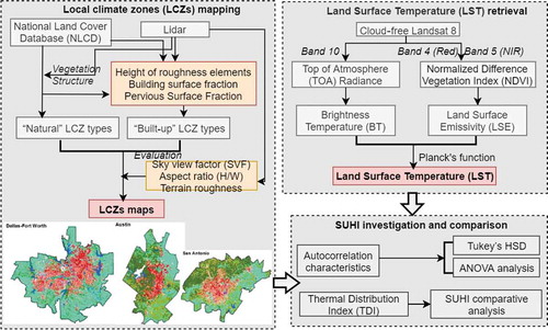
Figure 2. Workflow for linking land surface temperature (LST) to Local Climate Zones (LCZs) for the SUHI investigation

“Built-up” LCZ types are mostly concentrated in the center of the study areas, especially for Dallas-Fort Worth. In terms of “natural” LCZ types, clustered patterns of LCZ D (low plants) are prominent, for both average size and total/summed area. LCZ D covers 43.20% and 29.56% of the total metropolitan areas of Dallas-Fort Worth and Austin, respectively. LCZ A (dense trees) appears frequently on the eastern side of the Austin metropolitan area, as well as in the northern area of San Antonio, showing a clear contrast with the pattern for LCZ D (low plants).

3. Methodology

The SUHI investigation process in this study was mainly conducted by linking Landsat-derived LST with LCZs. Figure 2 provides a graphical description of the workflow for LCZ mapping (Zhao et al. 2019), LST retrieval, and SUHI intensity analysis.

3.1. Surface temperature derivation

Landsat imagery has become the foremost source for fine-scale SUHI studies since 2008, when the entire data archive became freely available. Cloud-free daytime Landsat 8 images from one summer (20 July) and one winter (25 January) day in 2015 were obtained to calculate LST for the SUHI investigation. The Thermal Infrared Sensor (TIRS) onboard Landsat 8 measures LST in two thermal bands. For the TIRS, common algorithms for LST calculation include a radiative transfer equation (Hook et al. 2004), split-window algorithm (Jiménez-Muñoz et al. 2014), and single-channel algorithm (Jiménez-Muñoz et al. 2008). For this study, we used the Planck function method to calculate LST, owing to its demonstrated feasibility and optimal performance (Isaya Ndossi and Avdan 2016). Considering the larger calibration uncertainty and greater sensitivity to water vapor continuum absorption for band 11 (Coll et al. 2012; Yu et al. 2014), LSTs were computed based on band 10 (10.6–11.19 µm) for this study (Table 2).

Digital Numbers (DNs) were first converted to Top of Atmosphere (TOA) radiance$(L_{TOA,\lambda }$$(L_{TOA,\lambda }$), with Gain and Bias (or Offset) values from the imagery header files. These values were then transformed to at-sensor brightness temperature $(T_{sen})$$(T_{sen})$ in Kelvin (K):

(1) $T_{sen}=\frac{K2}{ln\left(\frac{K1}{L_{TOA,\lambda }}+1\right)}$$T_{sen}=\frac{K2}{ln\left(\frac{K1}{L_{TOA,\lambda }}+1\right)}$(1)

where K1 and K2 are TIRS calibration constants, which can be obtained from the header files.

Due to thermal variation of different land surface properties at the metropolitan level, Land Surface Emissivity (LSE) was used to correct$T_{sen}$$T_{sen}$. The Normalized Difference Vegetation Index (NDVI) threshold estimation algorithm (Sobrino et al. 1990; Sobrino et al. 2004) was applied in this study to calculate land surface emissivities for general cover types (Table 3).

Table 3. Land Surface Emissivity (LSE) assignment and calculation according to the NDVI threshold

NVDI range	Assumed land cover types	Land Surface Emissivity (LSE) value ($i.e.,\hspace{0.17em}{\epsilon }_{\lambda })$$i.e.,\hspace{0.17em}{\epsilon }_{\lambda })$
(−1, 0.2]	Developed/rock/soil dominant	${\epsilon }_{s\lambda }=$${\epsilon }_{s\lambda }=$0.966 (Yu et al. 2014)
(0.2, 0.5)	Combination of vegetation and rock/soil	(2) ${\epsilon }_{\lambda }={\epsilon }_{v\lambda }{P}_V+{\epsilon }_{s\lambda }(1-P_V)+C_{\lambda }$(2) (3) $C_{\lambda }=\left(1-{\epsilon }_{s\lambda }\right){\epsilon }_{v\lambda }{F}^{\prime }(1-P_V)$(3) (4) $P_V={\left[\frac{NDVI-NDV{I}_{min}}{NDV{I}_{max}-NDV{I}_{min}}\right]}^2$(4)
[0.5, 1)	Vegetation dominant	${\epsilon }_{v\lambda }=$${\epsilon }_{v\lambda }=$0.986 (Yu et al. 2014)

Note: ${\epsilon }_{v\lambda }\hspace{0.17em}$${\epsilon }_{v\lambda }\hspace{0.17em}$refers to vegetation emissivity and ${\epsilon }_{s\lambda }$${\epsilon }_{s\lambda }$ refers to soil emissivity. $P_V$$P_V$ is the vegetation fraction. $C_{\lambda }$$C_{\lambda }$ calibrates the cavity effect due to surface roughness, as explained in equation (3)(3) $C_{\lambda }=\left(1-{\epsilon }_{s\lambda }\right){\epsilon }_{v\lambda }{F}^{\prime }(1-P_V)$(3) , where $F^{\prime }$$F^{\prime }$ is a geometrical factor with a value of 0.55, considering geographical distributions (Sobrino et al. 1990).

At-sensor brightness temperature was transformed to LST using the Planck function (Equation 5(5) $Ts=\frac{Tsen}{1+\frac{\lambda Tsen}{\rho }ln{\epsilon }_{\lambda }}$$Ts=\frac{Tsen}{1+\frac{\lambda Tsen}{\rho }ln{\epsilon }_{\lambda }}$(5) )(Artis and Carnahan 1982; Isaya Ndossi and Avdan 2016).

(5) $Ts=\frac{Tsen}{1+\frac{\lambda Tsen}{\rho }ln{\epsilon }_{\lambda }}$$Ts=\frac{Tsen}{1+\frac{\lambda Tsen}{\rho }ln{\epsilon }_{\lambda }}$(5)

where $Ts$$Ts$ is LST in Kelvin (K), λ is the wavelength of emitted radiance (λ = 10.895 μm), and ρ (e.g., $\frac{h\ast c}{\sigma }$$\frac{h\ast c}{\sigma }$) = 1.438 × 10⁻² mK ($h$$h$is Planck’s constant and $c$$c$ is the speed of light).

As the meteorological conditions (e.g., synoptic situation) vary over the three metropolitan areas, we standardized the LST maps as the normalized surface temperatures for comparative analysis for the two study dates. The normalization method involved linear scaling using the Min-Max function to have LST values range between 0 and 1.

3.2. Applying LCZs for SUHI investigation

To explore the applicability of LCZs for SUHI analysis, we tested the hypothesis that LCZs can facilitate intra-zonal comparisons of SUHI phenomenon for the three study areas. To obtain independent samples for statistical tests, LST pixel values were sampled systematically at a distance of 270 m, which corresponded to the original LCZ mapping scale.

A one-way analysis of variance (ANOVA) was conducted to assess LST intra-zonal variation among different LCZs using the R programming environment. Since the F-values resulting from the ANOVA revealed that mean LST was different for at least one pair of the LCZs under investigation, we further identified specific (statistically significant) pairwise differences in mean LST by employing a post hoc Tukey’s Honest Significant Difference (HSD) test for the three metropolitan areas.

To make comparisons in terms of SUHI phenomenon between LCZs within a single area and comparisons among the study areas, we used the Thermal Distribution Index (TDI) to estimate the extent to which each LCZ contributes to the heating effect of the SUHI in each of the metropolitan areas (Zhao 2018). Here, the area proportion of “hot” LST pixels in the four LST classes (i.e., “hot,” “sub-hot,” “sub-low,” and “low”) defined by Jenks natural breaks, were used as an indicator of the SUHI intensity.

(6) $TD{I}_{LC{Z}_i}=\frac{AHig{h}_{LC{Z}_i}/A_{LC{Z}_i}}{AHigh/A}$$TD{I}_{LC{Z}_i}=\frac{AHig{h}_{LC{Z}_i}/A_{LC{Z}_i}}{AHigh/A}$(6)

where $TD{I}_{LCZi}$$TD{I}_{LCZi}$ is the distribution frequency of high LST pixels for an $LC{Z}_i$$LC{Z}_i$. $AHig{h}_{LC{Z}_i}$$AHig{h}_{LC{Z}_i}$ refers to the area with high LST pixels, while $A_{LC{Z}_i}$$A_{LC{Z}_i}$ is the area of a single LCZ (e.g., LCZ 1, LCZ 2, … LCZ G). $AHigh$$AHigh$ is the area of the high LST pixels of the entire study area (A). A $TD{I}_{LC{Z}_i}$$TD{I}_{LC{Z}_i}$ value of 1 represents an average contribution of the $LC{Z}_i$$LC{Z}_i$to the overall SUHI phenomenon. Therefore, if the $TD{I}_{LC{Z}_i}$$TD{I}_{LC{Z}_i}$ was greater than 1, there was a heating effect of $LC{Z}_i$$LC{Z}_i$, while if the value of $TD{I}_{LC{Z}_i}$$TD{I}_{LC{Z}_i}$ was less than 1, $LC{Z}_i$$LC{Z}_i$ showed a cooling effect on the entire metropolitan area.

4. Results

4.1. Spatial distributions of LST and LCZs

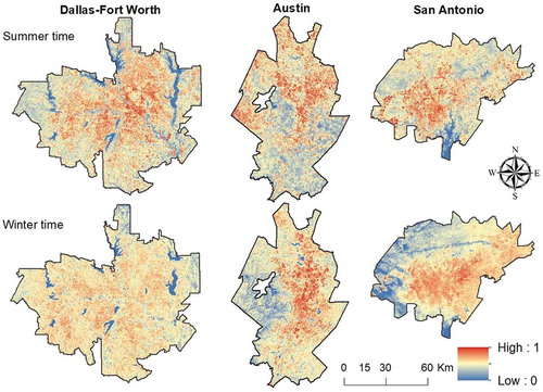
Figure 3 shows an example of the spatial distribution of standardized LST. Overall, there was an obvious SUHI phenomenon on 20 July 2015 for all three metropolitan areas, indicated by the similar characteristics of the LST spatial distributions. As expected, hotspots of LST were located primarily in the downtown and adjacent urban areas and were often associated with the distribution of built-up land. Low surface temperatures occurred along the central western side of Austin and in northern San Antonio, where the topography is more complex and large forested areas remain intact. The lowest LSTs were associated with waterbodies (e.g., Dallas-Fort Worth). The SUHI phenomenon on 25 January 2015 was not as obvious as the July analysis, especially for Dallas-Fort Worth, although high surface temperatures occurred in the downtown areas of Austin and San Antonio.

Figure 3. Spatial distributions of normalized land surface temperature (LST) in the three study areas one summer (20 July) and one winter (25 January) day in 2015

4.2. Result for linking LST with LCZ mapping

The statistical distribution of LST in individual LCZ classes indicated varying thermal characteristics among LCZs (Figure 4). Our LCZs mapping scheme, especially applying spatial scale of 90 m for LCZs properties generation, failed to detect LCZ 8 to match the ground illustrations from Google Earth. We excluded LCZ 8 (large low-rise) in the following analysis as well as LCZ 7 (lightweight low-rise) owing to its low frequency of occurrence in the study areas. In accordance with the above finding regarding LST patterns, the LSTs for “built-up” types (LCZs 1–10) were generally higher than those for “natural” cover types (LCZs A–G) in all three metropolitan areas. These qualitative LST patterns for LCZs were generally consistent among the three metropolitan areas, despite their quantitative differences in terms of absolute LST values. In short, LCZ mapping facilitated the differentiation of urban morphology characteristics within unique climate regions.

Figure 4. Box-plots of land surface temperature values for Local Climate Zones (LCZs) in three Texas metropolitan areas on the late morning of 25 January 2015 (in red) and 20 July 2015 (in blue)

(Notes: The bottom and top line of the boxes represent the first quartile (Q1) and the third quartile (Q3), respectively. The line in the box is the median value. The height of the box is the interquartile range (IQR). The top whisker denotes either the maximum value or (Q3 + 1.5*IQR), whichever is smaller. The bottom whisker denotes either the minimum value or (Q1– 1.5*IQR), whichever is larger.)

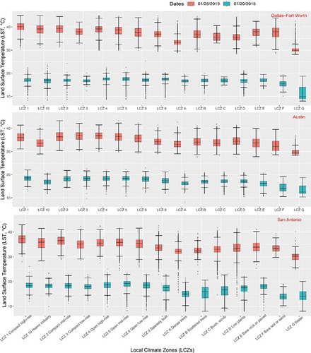
On 20 July 2015 during satellite overpass, LCZ 1 (compact high-rise) was the warmest zone, followed by LCZ 4 (open high-rise; except in Austin). We also observed LST variations among LCZs with various building densities. For example, “compact” LCZ types showed higher surface temperatures than the more “open” LCZ types (e.g., LCZ 1 versus LCZ 4; LCZ 2 versus LCZ 5, LCZ 3 versus LCZ 6), especially in Dallas-Fort Worth and Austin. Additionally, the “open” LCZ types were generally warmer than LCZ 9 (sparsely built). Figure 4 demonstrates that “high-rise” LCZ types exhibited the highest median LST, followed by “mid-rise” (e.g., LCZ 2 versus LCZ 5) and “low-rise” types. LCZ 10 (heavy industry) exhibited an entirely different distribution in each of the three study areas. LCZ G (water) was the coolest zone for all three metropolitan areas, followed by LCZ A (dense trees) and LCZ F (bare soil or sand). LCZ 9 (sparsely built) was cooler than some “natural” LCZ types (e.g., LCZ E, LCZ F) for San Antonio and Dallas-Fort Worth and cooler than LCZ D (low plants) for Austin.

On 25 January 2015 during satellite overpass, the LST differences among LCZs were less apparent than those in summer and the LST range within each LCZ was smaller and included fewer outliers. Unlike the LST distribution in summer, the highest SUHI intensities were observed in LCZ 4–6 “open” types, especially for Dallas-Fort Worth and for San Antonio. In Austin, the highest LSTs (>10°C) were found for LCZ 1, LCZ 4, LCZ 3, LCZ 5, and LCZ 2, and a moderately lower SUHI intensity occurred in LCZ 9. Like the SUHI on 20 July 2015, LCZ G (water) had the lowest average surface temperature for the three study areas, followed by LCZ F (bare soil or sand). LCZ D (low plants) showed a pronounced different rank order, with a slightly higher median LST among all the zones. However, the LST difference between LCZ G (water) and the other LCZs was smaller in winter than on 20 July 2015 for Austin and San Antonio.

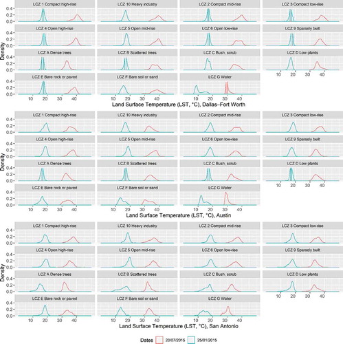
LST values were further evaluated based on distribution density for each LCZ to ensure the assumption of normality was met for the subsequent ANOVA (Figure 5). LST distributions were generally Gaussian except LCZ F for Austin and LCZ G for all three metropolitan areas. LCZ G demonstrated substantial variation and multi-modal distribution, with a significant departure from the mean LST. The homogeneity of variance assumption was not satisfied in the ANOVA; however, a nonparametric Kruskal-Wallis (K-W) test (Kruskal and Wallis 1952) and post hoc Conover tests (Conover and Iman 1979) produced results that were qualitatively the same as the one-way ANOVA F-test and Tukey’s HSD. Therefore, the former (parametric) results are presented. The results of the ANOVA indicated statistically significant differences in average LST among LCZs.

Figure 5. Density distributions of land surface temperature (LST) values for individual Local Climate Zones (LCZs) for the three metropolitan areas in Texas, USA

Results from the Tukey HSD tests are provided in Figure 6. Grey shading for a pair of LCZs means that they did not show significant differences in terms of LST. Most pairs of LCZs showed significant differences in mean LST on both 25 January 2015 and 20 July 2015, with high significance levels. This suggests that LCZs helped identify distinctive, relatively homogeneous LST zones. On 20 July 2015, there were 78, 82, and 81 pairs of LCZs indicating statistically significant LST differences for Dallas-Fort Worth, Austin, and San Antonio, respectively (i.e., 85.71%, 90.11%, and 89.01%). On 25 January 2015, there were 80.02%, 90.11%, and 87.9% pairs of LCZs indicating differences, slightly lower than in summer. The difference between pairs of LCZs were more apparent in Austin and San Antonio than in Dallas-Fort Worth, especially in winter (Figure 6).

Figure 6. Tukey Honestly Significant Difference test for the difference in land surface temperature (LST) for pairs of Local Climate Zones (LCZs)

(Notes: Boxes in gray denote no significant difference between the corresponding LCZs. Boxes in dark red, red, and light red indicate that the mean value of the column LCZ is significantly higher than that of the row LCZ, at the 0.001, 0.01, and 0.05 level, respectively. Boxes in dark green, green, and light green indicate that the mean value of the column LCZ is significantly lower than that of the row LCZ, at the 0.001, 0.01, and 0.05 level, respectively.)

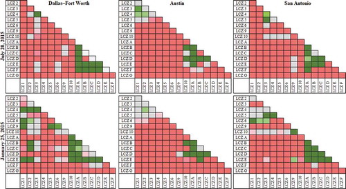
Combined, the results suggest that for the three metropolitan areas, LCZ 4 (open high-rise), LCZ 5 (open mid-rise), LCZ 6 (open low-rise), LCZ 10 (heavy industry), LCZ A (dense trees), LCZ B (scattered trees), LCZ D (low plants), and LCZ G (water) had the most discriminatory power for identifying different LST zones, both in summer and winter. For Dallas-Fort Worth, LCZ E and LCZ F were not significantly different from each other in summer or winter. Additionally, there were not significant differences for some of the “built-up” LCZ types in summer in terms of surface temperature. Noticeably, LCZ F (bare soil or sand) was indistinguishable from LCZ C (bush, scrub) and LCZ D (low plants) for Dallas-Fort Worth and from LCZ B (scattered trees) for San Antonio in the winter. Overall, the “natural” LCZ types (A–G) were significantly different from each other in terms of LST.

In terms of the “built-up” LCZ types, for Dallas-Fort Worth, LSTs for LCZ 2 (compact mid-rise) and LCZ 3 (compact low-rise) could not be distinguished from other “open” LCZ types. For the zones in Austin, most of the “built-up” LCZ types were associated with significant pairwise differences in LST, except for LCZ 2, which was statistically indistinguishable from LCZ 1 (compact high-rise), LCZ 3 (compact low-rise), and LCZ 5 (open mid-rise) in summer. In winter, LCZ 1 was indistinguishable from several “built-up” LCZ types. For San Antonio, most LCZs showed that LSTs were distinguished very well in summer, especially for LCZ 9 (sparsely built) and LCZ 10 (heavy industry). Additionally, LCZ 1 and LCZ 4 were indistinguishable from “high-rise” LCZ types in winter. Taken together with the box-plots of LSTs in terms of LCZs (Figure 4), the thermal characteristics of LCZs showed noticeable seasonal variation.

4.3. Application of LCZs for SUHI investigation

We focused on the SUHI on 20 July 2015, because of the apparent effect of SUHIs, as well as the adverse impact of hot weather. TDI values related to “high” LST pixels were calculated to quantify the contributions of “hot” LST pixels from various LCZs within each study area, and to compare the relative contributions of specific LCZs in the different metropolitan areas (Figure 7). The TDI values further demonstrated the heterogeneity of LST values across the LCZs. Overall, the “built-up” cover types (LCZs 1–10) had TDI > 1 on 20 July 2015, except for LCZ 10 (heavy industry) and LCZ 9 (sparsely built) for Austin and LCZ 9 for San Antonio (Figure 7). The LCZ types “compact” and “open” and the types “high-rise and mid-rise” (LCZ 1, 2 and LCZ 4, 5) had severe heating impacts on the thermal environment, with TDI values ≥2 (Figure 7).

Figure 7. Thermal Distribution index (TDI) of high-surface-temperature centers for Local Climate Zones (LCZs) in three Texas metropolitan areas on 20 July 2015. (The full names of LCZs are provided in Figure 1. Red dashed lines indicate TDI = 2 and TDI = 1, respectively.)

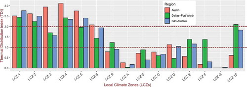
In contrast, the “natural” LCZ categories had TDI values <1 (Figure 7). Exceptions were LCZ D (low plants) (TDI = 1.13 for Austin, TDI = 1.04 for San Antonio), and LCZ E (bare rock or paved) (1.16 for San Antonio and 1.38 for Dallas-Fort Worth), although they were near a TDI value of 1. With respect to the role of individual LCZs on SUHI intensity, the effect of LCZ G (water) and LCZ A (dense trees) was close to 0, with values ranging from 0 to 0.25 (Figure 7). This finding can be interpreted as an overall lack of “high” surface temperature spots on the summer date of 20 July 2015 for these two LCZ types, indicating a clear cooling effect for the corresponding metropolitan areas.

Despite the general similarity in the tendency of a heating/cooling effect of corresponding LCZs, there were some noteworthy differences between the three metropolitan areas. LCZs of Austin demonstrated higher TDI variation than those of the other areas. Compared with LCZs in Dallas-Fort Worth and San Antonio, most of the “built-up” LCZ categories in Austin and some “natural” cover types (e.g., LCZ A dense trees; LCZ C bush, scrub; and LCZ D low plants) had higher TDI values, indicating a stronger heating effect.

Considering that the warm thermal environment in urbanized areas is due in part to the reduction of evapotranspiration by vegetation cover, the relationship of LST and NDVI has been explored in a number of studies to characterize the thermal behavior of urbanized areas (Bokaie et al. 2016; Lin and Wen 2011; Weng and Fu 2014; Weng, Lu, and Schubring 2004; Yue et al. 2007). We explored the relationship between LST and NDVI (calculated from the same Landsat 8 imagery) on 20 July 2015 to evaluate the thermal behavior of different LCZs. With a sufficient sample size and strong statistical significance (p < 0.001), the results of regression analysis showed a strong inverse correlation between mean LST and NDVI for different LCZs (Table 4).

Table 4. Linear regression results for the linear regression between LST and NDVI, separated by Local Climate Zone (LCZ), on 20 July 2015

LCZs	Regression coefficients			Coefficient of determinations (R^2)
	Dallas-Fort Worth	Austin	San Antonio	Dallas-Fort Worth	Austin	San Antonio
1	−10.13	−6.67	−8.73	0.23	0.30	0.30
2	−10.27	−7.61	−7.94	0.35	0.36	0.27
3	−10.19	−6.84	−6.85	0.37	0.30	0.23
4	−8.49	−6.76	−7.82	0.23	0.29	0.27
5	−8.64	−7.82	−8.22	0.24	0.29	0.22
6	−9.62	−8.12	−8.36	0.33	0.25	0.22
9	−8.86	−7.18	−9.02	0.18	0.16	0.22
10	−10.28	−8.97	−11.29	0.31	0.29	0.42
A	−8.88	−11.12	−9.79	0.23	0.33	0.15
B	−7.08	−9.50	−9.15	0.20	0.26	0.09
C	−17.81	−10.64	−10.38	0.54	0.28	0.15
D	−11.92	−8.73	−12.97	0.34	0.26	0.24

Note: 1) Please refer to the name of LCZs from Figure 4. 2). The LCZ E Bare rock, LCZ F Bare soil or sand, and LCZ G Water were excluded due to the low vegetation cover.

5. Discussion

5.1. Applicability of LCZs for SUHI characterization

With generally consistent findings for the three metropolitan areas, the significant differences in LST among LCZs demonstrates that LCZ mapping can facilitate the analysis of LST variations and is thus relevant for SUHI characterization, modeling, monitoring, and comparison.

First, the LCZs characterized by different land cover types (“built-up” types and individual “natural” types) showed the highest LST variations. For example, due to the high thermal heat capacity of water relative to other properties, LCZ G was found to be the coolest, with a surface temperature around 27°C in summer. LCZ A (dense trees) had the next lowest average surface temperature and accounted for a considerable proportion of the landscape in Austin and San Antonio. Similar findings have been observed regarding LST variation among LCZs in the Yangtze River Delta, China (Cai et al. 2018) and in Prague, Brno, Czech Republic (Geletič, Lehnert, and Dobrovolný 2016). The variation in thermal behavior by different land use and land cover (LULC) types has been well documented for several areas since the 1970s (Amiri et al. 2009; Bokaie et al. 2016; Lazzarini, Marpu, and Ghedira 2013; Roth, Oke, and Emery 1989; Zhou et al. 2013). Together with these previous findings, the results of our study demonstrate the importance of LULC type in determining the spatial variation of LST.

Aside from LST variation between different land covers, one advantage of evaluating LST based on LCZs is that LCZ mapping simplifies complex urban morphology into relatively uniform temperature zones, especially for the “built-up” LCZ types (Stewart and Oke 2012). Regarding the effect of the heterogeneous character of the urbanized area on LST spatial variation, scholars have suggested that thermal behavior of urbanized landscapes can be explained by the various urban land uses and urban canopy structure, which should be accounted for in UHI phenomenon explanation (Carlson, Augustine, and Boland 1977; Goward 1981). The factors used to define LCZs, including the sky view factor (Chun and Guhathakurta 2017; Unger 2009), albedo (Levy 2016), and solar radiation absorption (Chun and Guldmann 2014), have all been reported to affect LST spatial variation and SUHI formation. This study further addressed the need to examine 3D urban morphological information with alternative parameters to derive a uniform zone in order to accurately report LST spatial variation and to render the results comparable.

The LST and NDVI regression coefficient (−6.67 to −11.80) differed among LCZs, showing the same pattern in the three metropolitan areas. This finding indicates that distinct thermal environments were formed in different LCZs. Here, LCZ C (bush, scrub) in Dallas-Fort Worth showed a strong correlation with LST, which explained its strong cooling effect during hot weather in summer, in contrast to the slight heating effect from LCZ C for the other two metropolitan areas (Table 4). It is noteworthy that the LCZ C of Dallas-Fort Worth corresponded to shrub and scrub along the river corridor, characterized by high soil moisture, which run through the urban areas. Considering that the soil moisture is a subscript classifier for variable land cover properties (Table 2 in Stewart and Oke 2012) and its effect on the LST–NDVI curve (Goward, Xue, and Czajkowski 2002; Weng, Lu, and Schubring 2004), soil moisture should be further explored in future LCZ-LST studies.

5.2. Uncertainties of LCZ mapping for SUHI analysis

For each specific metropolitan area, there were several LCZs that could not be clearly distinguished in terms of their LSTs, including LCZ 3 (compact low-rise), LCZ E (bare rock, or paved), and LCZ F (bare soil or sand). This phenomenon can partly be explained by the limitations of the LCZ mapping in this study. With a relatively small contribution, LCZ E and LCZ F showed different normalized mean surface temperatures and heating/cooling effects among the three metropolitan areas. In addition, LCZ F had the largest LST variation. This is partly because the GIS-based LCZ mapping emphasized the morphological characteristics rather than the surface materials (Zhao et al. 2019). For example, LCZ E included two land cover types: bare rock and paved. Further, the interpretation of satellite imagery from Google Earth indicated that substantial parts of areas of bare rock and paved land belonged to transportation-related impervious surfaces.

It should be noted that the parking lots, airports, transportation hubs, etc., normally belong to LCZ 8 (large low-rise) if they feature large, low buildings. Nevertheless, the surface of bare rock and impervious material can have different thermal behaviors during the late morning, when Landsat passed over the study areas. The large low-rise buildings can be common observed in different places worldwide, including Dallas, Austin, and San Antonio. The large low-rise buildings can be mixed with green or impervious surface in various landscape conditions, and the surface water and energy balances can be different. In the daytime, the LCZ 8 with considerable impervious material can be the warmest zone, due to large horizontal rooftops that are irradiated and warm. As such, the LCZ 8 should therefore not be “aggregated” with surrounding landscapes in the LCZs mapping process, since SUHI management strategies for LCZ 8 would be much different than for other LCZ classes.

In terms of “natural” LCZ types, a study by Geletič et al. (2019) suggested benefits of a further sub-classification, due to the impact of vegetation characteristics on intra-zonal LCZ variation. Our findings confirm that there are other features (i.e., vegetation volume and health conditions) that potentially determine the LST, leading to intra-LCZ variations.

LCZ 10 (heavy industry) had different thermal characteristics in the three metropolitan areas, which is in contrast with other LCZs. Partly, this is because LCZ 10 was also sparsely distributed throughout Dallas-Fort Worth and to some extent in San Antonio. Some areas of LCZ 10 were adjacent to the “natural” LCZ types. As we delineated LCZ 10 based on city planning data (Zhao et al. 2019), which did not include the emissions of anthropogenic heat, this may have led to the unexpected findings for LST distribution. Thus, attention should be paid for LCZ mapping accuracy and the assignment of urban areas to the correct LCZs.

The uncertainties of LCZ mapping for SUHI investigations is also related to the issue of scale. The common characteristics of LCZs with indistinguishable LSTs were their small area proportion and high fragmentation, which affected their thermal characteristics due to contributions from adjacent land covers. For LCZ mapping, LCZs were defined as areas with uniform land cover and structure, construction materials, and human activity. However, each LCZ was not a completely homogeneous zone, and the boundaries between them were not clear. As samples for analysis, we used the LST values at the pixel level, which might be located nearby the LCZ boundaries. In addition, some surface properties may show heterogeneous thermal variations at a scale smaller than the LCZs. For example, Zhang et al. (2009) reported that smaller patches of vegetated area provided less cooling than larger vegetated patches. In this study, several outliers of LCZ A (dense trees) showed high surface temperatures. A similar result was also observed by Geletič, Lehnert, and Dobrovolný (2016). In short, LCZ delineation requires a compromise between universal applicability and local accuracy.

For the “compact” types (LCZ 1–3), buildings have a more pronounced effect of reducing solar radiation and increasing shadowing in the street canyons in the selected winter day. This finding is consistent with those from other studies (Huang and Wang 2019; Theeuwes et al. 2014). In addition, due to the differences of biomes and ecological regions, the vegetation metabolism is very weak in winter, with decreased evapotranspiration, which leads to a smaller cooling effect in the “natural” LCZ types. This is supported by the fact that Dallas-Fort Worth was much colder on 25 January 2015, (approximately 10°C lower in 2010–2019, Table 1) than the other two areas.

In this work, only two morning LSTs derived from satellite imagery were used for SUHI study considering the clear sky conditions. Therefore, the seasonal characteristics of the SUHI for the study areas could not be generalized. Also, the climatological characteristics (e.g. wind, cloud, humidity) can be different among the three study areas, which impedes the thermal comparison of their LCZ mapping. Additionally, the late morning satellite overpass and subsequent calculation of LST is of limitation when detecting the spatial distribution of heat-health risks compared with temperature acquired during another time of the day (i.e., an afternoon temperature with solar heat effect). While all the study areas showed a less distinguishable SUHI effect on 25 January 2015 than that on 20 July 2015, it is not convincing to give a general statement on the seasonal SUHI phenomenon based on this research. Our study therefore further indicated that the necessity of applying time-series imagery to study the seasonality of heat island effects.

The LCZs mapping uncertainty arising from LCZs mapping unit selection and scheme is another limitation of applying LCZs for SUHI study. The final spatial scale of 270 meters was chosen as the final LCZs mapping unit, which includes several aggregations. For example, the Lidar data had a native spatial accuracy within 1 meter, and two aggregation steps were performed to aggregate from fine scale to coarse scale. A spatial resolution of 90 m was considered for LCZs properties generation to keep the accuracy and details of the LCZs properties (i.e., buildings character) at as fine a scale as possible. The final aggregation (270 m × 270 m) had to be conducted to match the LCZs definition and avoid too excessive heterogeneity. Furthermore, in order to keep some types of LCZs that appeared in very small proportions, an aggregation rule was implemented such that LCZ n (0 < n ≤ 10) would have higher priority than LCZ n + 1 (0 < n ≤ 10) if there were more than two pixels for LCZ n. Thus, LCZ 4 may take advantage of the surrounding LCZ 5 and the imagery illustration of LCZ 4 can be somehow different from the illustrations from Stewart and Oke (2012).

Additionally, building surface fraction, pervious surface fraction, and height of roughness features, mainly calculated from the Lidar dataset, were main properties for mapping LCZs (Zhao et al. 2019). For instance, although cut-down, values from Stewart and Oke (2012) were used for LCZs mapping, different data sources, calculation methods and strategies could also lead to low mapping frequency of LCZ 8 (large low-rise) compared to other studies (Taubenboch et al. 2020). Nevertheless, the common LCZ 8 in U.S. cities (i.e., warehousing, shopping malls, large parking lots, etc.) were found to be warm areas during the day, and could even can be warmer than high-rise downtown areas according to Imhoff et al. (2010).

5.3. The effect of LCZs on SUHI formation

With a uniform LCZ classification scheme, this study provides strong evidence that LCZ mapping can be replicable for comparative analysis of the SUHI phenomenon. The TDI of high surface temperatures further demonstrates that the LCZ mapping results can efficiently facilitate intra- and inter-zone comparisons of SUHI intensity. Generally, the overall SUHI effect was primarily caused by the heating effect of built-up land cover. Furthermore, this study indicates that some LCZs in different regions contribute to opposite heating/cooling effects (e.g., LCZ 9 sparsely built, LCZ D low plants).

Furthermore, the effects of the spatial distribution of LCZs on SUHI intensity need to be studied in greater detail. The distributions of LCZs reflected the varying spatial arrangements of natural and built-up environments, which in turn affected the spatial variations of LST. It is important to recognize that the LCZs in the Dallas-Fort Worth metropolitan area showed a lower capability to track the LST variation throughout the region (Figure 7). Compared with Austin and San Antonio (Figure 1(c–d)), Dallas-Fort Worth had a distinct spatial heterogeneity of “natural” LCZ types, due to the geographical location and climatic condition. In particular LCZ D (low plants) and LCZ G (water) intersected with LCZs 1–10 (“built-up” types), with the highest proportion occurring in Dallas-Fort Worth compared with the composition in the other two metropolitan areas. These natural cover types separated urbanized areas of Dallas-Fort Worth into several major city centers (e.g., Arlington, Irving), playing the role of city “corridors” (Figure 1(b)).

Supplementary examination of the LCZs with Google Earth indicated that the main river and stream basins led to the formation of a strip of LCZ D and LCZ G, neighboring with built-up land (LCZ 4 and LCZ 5) (Zhao et al. 2019). This arrangement of LCZs in Dallas was in agreement with the LSTs in terms of the small number of LST outliers in LCZs 4 and 5 (open high-rise and open mid-rise) and in LCZ D (low plants) and the large number of LST outliers in LCZ G (water). This intersection effect by different LCZs can also help explain other outliers (e.g., LST in LCZ 9 and LCZ A of San Antonio). A recent study of Wuhan, China also indicated that the landscape layout of LCZs was an important factor in SUHI formation (Wang, Zhan, and Ouyang 2017). Spatial heterogeneity and scale characteristics have also been addressed in other SUHI studies (Zhao et al. 2018; Zhou, Huang, and Cadenasso 2011). Further studies on the spatial heterogeneity and scale characteristics of LCZs are needed to lead to comprehensive findings for the SUHI phenomenon of our study regions. Besides, the surface temperature measurement is biased to horizontal surfaces (mainly rooftops in urban areas) without correction for 3-D geometric and thermal anisotropy effects, which are especially important to investigate complex “built” LCZs (Krayenhoff and Voogt 2016; Voogt and Oke 1998). Studies on estimating urban air temperature based on remotely sensed surface temperature have been conducted (Dos Santos 2020; Yoo et al. 2018), but its applicability in 3-D air temperature investigation still need evaluation.

The GIS-based LCZ delineation considered the inclusion of detailed landscape and morphology information for buildings and vegetation in entire metropolitan areas. Considering that our aims of LCZ mapping were to investigate SUHI, LCZs were defined on the basis of surface characteristics, which are relatively fixed, seasonally, and inter-annually. However, some types of vegetation cover are more responsive to climate and environmental conditions and more likely to change over time, leading to different heating/cooling effects for the corresponding LCZ. The thermal rank order of LCZs in different times of the year is consistent with results from other cities worldwide in terms of the seasonal thermal variation of LCZs (Geletič et al. 2019; Hu et al. 2019; Nassar, Blackburn, and Whyatt 2016). Thus, a larger sample of LSTs during nighttime and in different seasons would contribute to a more complete understanding of the overall relationship between LCZs and LST.

6. Conclusions

In this study, we assessed the utility of LCZs for the comparative analysis of LST spatial variations and analyzed how different LCZs affect the SUHI phenomenon. The observed relationship between LCZs and LST demonstrates that LCZ maps can be applied to investigate SUHIs and to complete comparative analyses of SUHIs in different localities and times. With the sufficient 3D urban morphological information available, this study provides strong evidence that LCZ mapping can provide a guideline to synthesize SUHI studies. It considers the LST distinctions among LCZ classes instead of between the conventional “urban” and “rural” land covers. The LCZ maps used in this study were delineated based mainly on the height of roughness features, building confliction and configuration, permeable surface proportion, and city land use planning codes and datasets. This study further points to the heterogeneity of built-up land in the urban environment; thus, different “built-up” LCZ types also showed different LST characteristics.

Our findings demonstrate the benefits of LCZ mapping for understanding the spatial variations of SUHIs. The intra-urban surface temperature comparison among different LCZs contributes to our knowledge of the influence of heterogeneous urban environments on the SUHI phenomenon. With the tools used in this study, urban planning and policymakers can better understand the effects of vegetation characteristics in individual LCZs at different times of the year, in order to develop urban green and other mitigation strategies for reducing the effect of heat islands. Furthermore, the LCZs and related LST datasets can contribute to climatic simulations with numeric models to better understand urban warming in the context of global climate change.

Disclosure statement

No potential conflict of interest was reported by the authors.

Appendix

Table A1. The spatial characteristics of individual LCZ patch size and overall LCZs pattern diversity for Austin, Dallas-Fort Worth, and San Antonio metropolitan areas

Statistical summary of individual patch of LCZs (unit: ha)
	Minimum patch size				Maximum patch size				Average patch size				Sum of patch size			Standard deviation
	Austin	Dallas-Fort Worth	San Antonio		Austin	Dallas-Fort Worth	San Antonio		Austin	Dallas-Fort Worth	San Antonio		Austin	Dallas-Fort Worth	San Antonio	Austin	Dallas-Fort Worth	San Antonio
LCZ 1	7.29	7.29	7.29		189.54	568.62	145.80		14.24	15.40	13.33		4016.79	13,333.41	2945.16	18.27	24.16	13.15
LCZ 2	7.29	7.29	7.29		43.74	43.74	87.48		11.42	10.51	13.67		2238.03	4519.80	4906.17	6.35	5.95	12.28
LCZ 3	7.29	7.29	7.29		43.74	36.45	247.86		11.98	9.62	17.94		1377.81	962.28	3426.30	7.55	4.50	25.04
LCZ 4	7.29	7.29	7.29		1822.50	20,885.80	466.56		33.71	51.15	21.39		27,206.28	112,936.63	14,441.49	106.06	475.22	36.20
LCZ 5	7.29	7.29	7.29		328.05	1013.31	8164.80		18.80	21.30	39.91		15,017.40	55,950.75	42,500.70	24.06	44.78	261.98
LCZ 6	7.29	7.29	7.29		102.06	422.82	225.99		14.71	16.49	17.13		11,736.90	55,068.66	25,981.56	12.03	20.50	17.70
LCZ 7	7.29	7.29	7.29		29.16	7.29	14.58		13.12	7.29	8.50		65.61	21.87	51.03	9.50	0.00	2.98
LCZ 8	7.29	7.29	7.29		51.03	29.16	65.61		13.34	9.24	12.35		1720.44	656.10	2704.59	9.78	4.60	9.27
LCZ 9	7.29	7.29	7.29		4476.06	9163.53	1246.59		52.53	71.96	33.94		50,687.37	167,312.79	51,481.98	199.32	457.99	86.22
LCZ 10	7.29	7.29	7.29		116.64	298.89	444.69		24.60	22.68	41.66		196.83	8594.91	1749.60	37.57	31.42	74.02
LCZ 11	7.29	7.29	7.29		27,220.90	1895.40	35,094.10		115.31	29.34	147.06		114,613.42	66,280.68	107,651.49	976.96	77.84	1820.88
LCZ 12	7.29	7.29	7.29		153.09	153.09	211.41		12.59	11.84	14.72		9076.05	12,961.62	3739.77	13.61	11.39	22.24
LCZ 13	7.29	7.29	7.29		10,300.80	51.03	4461.48		51.25	14.12	46.12		66,528.57	225.99	76,705.38	406.63	11.44	174.48
LCZ 14	7.29	7.29	7.29		43,579.60	207,328.00	15,491.30		107.68	301.61	104.06		133,632.98	416,521.88	107,389.08	1321.74	6093.21	774.08
LCZ 15	7.29	7.29	7.29		794.61	1151.82	225.99		17.60	18.90	16.96		2551.50	8959.41	3069.09	66.56	68.78	30.54
LCZ 16	7.29	7.29	7.29		648.81	167.67	459.27		35.84	22.00	43.60		2974.32	1275.75	2223.45	76.30	31.18	91.28
LCZ 17	7.29	7.29	7.29		1705.86	7960.68	1516.32		49.57	137.96	59.28		7931.52	38,629.71	3615.84	188.14	721.44	209.32
Overall LCZs pattern diversity
				Austin				Dallas-Fort Worth				San Antonio
Shannon’s Evenness Index				0.68				0.64				0.72

Note: The calculation is based on an LCZ raster dataset with a 270-meter pixel scale. The statistical summary of the Minimum, Maximum, Average, Sum, and Standard deviation is based on individual LCZ patches, while the overall LCZs pattern diversity is implied by Shannon’s Evenness Index, e.g., the relative abundance of different LCZ patch types. All indices were calculated with Fragstats, a spatial landscape pattern analysis Program (www.umass.edu/landeco/research/fragstats/fragstats.html).

References

- Amiri, R., Q. Weng, A. Alimohammadi, and S. K. Alavipanah. 2009. “Spatial–temporal Dynamics of Land Surface Temperature in Relation to Fractional Vegetation Cover and Land Use/cover in the Tabriz Urban Area, Iran.” Remote Sensing of Environment 113 (12): 2606–2617. doi:10.1016/j.rse.2009.07.021.
- Artis, D. A., and Walter H. C. 1982. “Survey of emissivity variability in thermography of urban areas.” Remote sensing of Environment 12 (4): 313–329.
- Austin City Council. 2012. “Imagine Austin Comprehensive Plan.” Austin City Council
- Barlow, J. F. 2014. “Progress in Observing and Modelling the Urban Boundary Layer.” Urban Climate 10 (Part 2): 216–240. doi:10.1016/j.uclim.2014.03.011.
- Boice, D. C., Michelle E. Garza, and Susan E. Holmes. 2018. “The Urban Heat Island of San Antonio, Texas, from 1991 to 2010.” In Journal of Geography, Environment and Earth Science International 17, no.2: 1–13.
- Bokaie, M., M. K. Zarkesh, P. D. Arasteh, and A. Hosseini. 2016. “Assessment of Urban Heat Island Based on the Relationship between Land Surface Temperature and Land Use/Land Cover in Tehran.” Sustainable Cities and Society 23: 94–104. doi:10.1016/j.scs.2016.03.009.
- Buyantuyev, A., and J. Wu. 2009. “Urban Heat Islands and Landscape Heterogeneity: Linking Spatiotemporal Variations in Surface Temperatures to Land-cover and Socioeconomic Patterns.” Landscape Ecology 25: 17–33.
- Cai, M., C. Ren, and Y. Xu 2017. “Investigating the Relationship between Local Climate Zone and Land Surface Temperature.” In 2017 Joint Urban Remote Sensing Event (JURSE), Dubai, United Arab Emirates. 1–4.
- Cai, M., C. Ren, Y. Xu, K. K.-L. Lau, and R. Wang. 2018. “Investigating the Relationship between Local Climate Zone and Land Surface Temperature Using an Improved WUDAPT methodology–A Case Study of Yangtze River Delta, China.” Urban Climate 24: 485–502. doi:10.1016/j.uclim.2017.05.010.
- Carlson, T., J. Augustine, and F. Boland. 1977. “Potential Application of Satellite Temperature Measurements in the Analysis of Land Use over Urban Areas.” In Bulletin of the American Meteorological Society, 1301–1303. American Meteorological Society.
- Chun, B., and J.-M. Guldmann. 2014. “Spatial Statistical Analysis and Simulation of the Urban Heat Island in High-density Central Cities.” Landscape and Urban Planning 125: 76–88. doi:10.1016/j.landurbplan.2014.01.016.
- Chun, B., and S. Guhathakurta. 2017. “The Impacts of Three-dimensional Surface Characteristics on Urban Heat Islands over the Diurnal Cycle.” The Professional Geographer 69 (2): 191–202. doi:10.1080/00330124.2016.1208102.
- City of Austin Neighborhood Planning and Zoning Department. 2008. “Austin Tomorrow Comprehensive Plan Interim Update.”
- Coll, C., Vicente C., Enric V., and Raquel N. 2012. “Comparison between different sources of atmospheric profiles for land surface temperature retrieval from single channel thermal infrared data.” Remote Sensing of Environment 117: 199–210.
- Conover, W. J., and R. L. Iman. 1979. On Multiple-comparisons Procedures, 1–17. NM, USA: Los Alamos Scientific Lab.
- Dallas City Council. 2006. “forwardDallas! Comprehensive Plan.”
- Darby, Lisa S., and C. J. Senff. 2007. “Comparison of the urban heat island signatures of two Texas cities: Dallas and Houston.” In Seventh Symposium on the Urban Environment (Expanded View). San Diego, CA
- Dos Santos, R. S. 2020. “Estimating Spatio-temporal Air Temperature in London (UK) Using Machine Learning and Earth Observation Satellite Data.” International Journal of Applied Earth Observation and Geoinformation 88: 102066. doi:10.1016/j.jag.2020.102066.
- Geletič, J., M. Lehnert, and P. Dobrovolný. 2016. “Land Surface Temperature Differences within Local Climate Zones, Based on Two Central European Cities.” Remote Sensing 8 (10): 788. doi:10.3390/rs8100788.
- Geletič, J., M. Lehnert, S. Savić, and D. Milošević. 2019. “Inter-/intra-zonal Seasonal Variability of the Surface Urban Heat Island Based on Local Climate Zones in Three Central European Cities.” Building and Environment 156: 21–32. doi:10.1016/j.buildenv.2019.04.011.
- Goward, S. N. 1981. “The Thermal Behavior of Urban Landscapes and the Urban Heat Island.” Physical Geography 2 (1): 19–33. doi:10.1080/02723646.1981.10642202.
- Goward, S. N., Y. Xue, and K. P. Czajkowski. 2002. “Evaluating Land Surface Moisture Conditions from the Remotely Sensed Temperature/vegetation Index Measurements: An Exploration with the Simplified Simple Biosphere Model.” Remote Sensing of Environment 79 (2–3): 225–242. doi:10.1016/S0034-4257(01)00275-9.
- Hidalgo, J., G. Dumas, V. Masson, G. Petit, B. Bechtel, E. Bocher, M. Foley, R. Schoetter, and G. Mills. 2019. “Comparison between Local Climate Zones Maps Derived from Administrative Datasets and Satellite Observations.” Urban Climate 27: 64–89. doi:10.1016/j.uclim.2018.10.004.
- Hook, S. J., G. Chander, J. A. Barsi, R. E. Alley, A. Abtahi, F. D. Palluconi, B. L. Markham, R. C. Richards, S. G. Schladow, and D. L. Helder. 2004. “In-flight Validation and Recovery of Water Surface Temperature with Landsat-5 Thermal Infrared Data Using an Automated High-altitude Lake Validation Site at Lake Tahoe.” IEEE Transactions on Geoscience and Remote Sensing 42 (12): 2767–2776. doi:10.1109/TGRS.2004.839092.
- Hu, J., Y. Yang, X. Pan, Q. Zhu, W. Zhan, Y. Wang, W. Ma, and W. Su. 2019. “Analysis of the Spatial and Temporal Variations of Land Surface Temperature Based on Local Climate Zones: A Case Study in Nanjing, China.” IEEE Journal of Selected Topics in Applied Earth Observations and Remote Sensing 12 (11): 4213–4223. doi:10.1109/JSTARS.2019.2926502.
- Hu, L., and N. A. Brunsell. 2015. “A New Perspective to Assess the Urban Heat Island through Remotely Sensed Atmospheric Profiles.” Remote Sensing of Environment 158: 393–406. doi:10.1016/j.rse.2014.10.022.
- Huang, X., and Y. Wang. 2019. “Investigating the Effects of 3D Urban Morphology on the Surface Urban Heat Island Effect in Urban Functional Zones by Using High-resolution Remote Sensing Data: A Case Study of Wuhan, Central China.” ISPRS Journal of Photogrammetry and Remote Sensing 152: 119–131. doi:10.1016/j.isprsjprs.2019.04.010.
- Imhoff, M. L., P. Zhang, R. E. Wolfe, and L. Bounoua. 2010. “Remote Sensing of the Urban Heat Island Effect across Biomes in the Continental USA.” Remote Sensing of Environment 114 (3): 504–513. doi:10.1016/j.rse.2009.10.008.
- Isaya Ndossi, M., and Ugur A. 2016. “Application of open source coding technologies in the production of land surface temperature (LST) maps from Landsat: a PyQGIS plugin.” Remote sensing 8 (5): 413.
- Jiménez-Muñoz, J. C., J. Cristóbal, J. A. Sobrino, G. Sòria, M. Ninyerola, and X. Pons. 2008. “Revision of the Single-channel Algorithm for Land Surface Temperature Retrieval from Landsat Thermal-infrared Data.” IEEE Transactions on Geoscience and Remote Sensing 47 (1): 339–349. doi:10.1109/TGRS.2008.2007125.
- Jiménez-Muñoz, J. C., J. A. Sobrino, D. Skoković, C. Mattar, and J. Cristóbal. 2014. “Land Surface Temperature Retrieval Methods From Landsat-8 Thermal Infrared Sensor Data.” IEEE Geoscience and Remote Sensing Letters 11 (10): 1840–1843. doi:10.1109/LGRS.2014.2312032.
- Khamchiangta, D., and S. Dhakal. 2019. “Physical and Non-physical Factors Driving Urban Heat Island: Case of Bangkok Metropolitan Administration, Thailand.” Journal of Environmental Management 248: 109285. doi:10.1016/j.jenvman.2019.109285.
- Kim, J.-H., D. Gu, W. Sohn, S.-H. Kil, H. Kim, and D.-K. Lee. 2016. “Neighborhood Landscape Spatial Patterns and Land Surface Temperature: An Empirical Study on Single-family Residential Areas in Austin, Texas.” International Journal of Environmental Research and Public Health 13 (9): 880. doi:10.3390/ijerph13090880.
- Koc, C. B., P. Osmond, A. Peters, and M. Irger. 2018. “Understanding Land Surface Temperature Differences of Local Climate Zones Based on Airborne Remote Sensing Data.” IEEE Journal of Selected Topics in Applied Earth Observations and Remote Sensing 11 (8): 2724–2730. doi:10.1109/JSTARS.2018.2815004.
- Kotharkar, R., and A. Bagade. 2018. “Evaluating Urban Heat Island in the Critical Local Climate Zones of an Indian City.” Landscape and Urban Planning 169: 92–104. doi:10.1016/j.landurbplan.2017.08.009.
- Krayenhoff, E. S., and J. A. Voogt. 2016. “Daytime Thermal Anisotropy of Urban Neighbourhoods: Morphological Causation.” Remote Sensing 8 (2): 108. doi:10.3390/rs8020108.
- Kruskal, W. H., and W. A. Wallis. 1952. “Use of Ranks in One-criterion Variance Analysis.” Journal of the American Statistical Association 47 (260): 583–621. doi:10.1080/01621459.1952.10483441.
- Lambin, E. F., B. L. Turner, H. J. Geist, S. B. Agbola, A. Angelsen, J. W. Bruce, O. T. Coomes, R. Dirzo, G. Fischer, and C. Folke. 2001. “The Causes of Land-use and Land-cover Change: Moving beyond the Myths.” Global Environmental Change 11 (4): 261–269. doi:10.1016/S0959-3780(01)00007-3.
- Landsberg, H. E. 1981. The Urban Climate. New York, NY: Academic press.
- Lazzarini, M., P. R. Marpu, and H. Ghedira. 2013. “Temperature-land Cover Interactions: The Inversion of Urban Heat Island Phenomenon in Desert City Areas.” Remote Sensing of Environment 130: 136–152. doi:10.1016/j.rse.2012.11.007.
- Levy, S. H. 2016. “Detecting Spatio-temporal Changes in Baltimore, Maryland’s Heat Island with Remote Sensing Imagery.”
- Lin, C.-H., and T.-H. Wen. 2011. “Using Geographically Weighted Regression (GWR) to Explore Spatial Varying Relationships of Immature Mosquitoes and Human Densities with the Incidence of Dengue.” International Journal of Environmental Research and Public Health 8 (7): 2798–2815. doi:10.3390/ijerph8072798.
- Liu, Z., C. He, Y. Zhou, and J. Wu. 2014. “How Much of the World’s Land Has Been Urbanized, Really? A Hierarchical Framework for Avoiding Confusion.” Landscape Ecology 29 (5): 763–771. doi:10.1007/s10980-014-0034-y.
- Mushore, T. D., T. Dube, M. Manjowe, W. Gumindoga, A. Chemura, I. Rousta, J. Odindi, and O. Mutanga. 2019. “Remotely Sensed Retrieval of Local Climate Zones and Their Linkages to Land Surface Temperature in Harare Metropolitan City, Zimbabwe.” Urban Climate 27: 259–271. doi:10.1016/j.uclim.2018.12.006.
- Nassar, A. K., G. A. Blackburn, and J. D. Whyatt. 2016. “Dynamics and Controls of Urban Heat Sink and Island Phenomena in a Desert City: Development of a Local Climate Zone Scheme Using Remotely-sensed Inputs.” International Journal of Applied Earth Observation and Geoinformation 51: 76–90. doi:10.1016/j.jag.2016.05.004.
- Oke, T. 1995. “The Heat Island of the Urban Boundary Layer: Characteristics, Causes and Effects.” In Wind Climate in Cities, 81–107. Dordrecht: Springer.
- Oke, T., and H. Cleugh. 1987. “Urban Heat Storage Derived as Energy Balance Residuals.” Boundary-Layer Meteorology 39 (3): 233–245. doi:10.1007/BF00116120.
- Oke, T. R. 1976. “The Distinction between Canopy and Boundary‐layer Urban Heat Islands.” Atmosphere 14: 268–277.
- Richard, Y., J. Emery, J. Dudek, J. Pergaud, C. Chateau-Smith, S. Zito, M. Rega, et al. 2018. “How Relevant are Local Climate Zones and Urban Climate Zones for Urban Climate Research? Dijon (France) as a Case Study.” Urban Climate 26: 258–274. doi:10.1016/j.uclim.2018.10.002.
- Roth, M., T. Oke, and W. Emery. 1989. “Satellite-derived Urban Heat Islands from Three Coastal Cities and the Utilization of Such Data in Urban Climatology.” International Journal of Remote Sensing 10 (11): 1699–1720. doi:10.1080/01431168908904002.
- San Antonio City Council. 2016. “SA Tomorrow Comprehensive Plan.”
- Schneider, A., M. A. Friedl, and D. Potere. 2010. “Mapping Global Urban Areas Using MODIS 500-m Data: New Methods and Datasets Based on ‘Urban Ecoregions’.” Remote Sensing of Environment 114 (8): 1733–1746. doi:10.1016/j.rse.2010.03.003.
- Shen, H., L. Huang, L. Zhang, P. Wu, and C. Zeng. 2016. “Long-term and Fine-scale Satellite Monitoring of the Urban Heat Island Effect by the Fusion of Multi-temporal and Multi-sensor Remote Sensed Data: A 26-year Case Study of the City of Wuhan in China.” Remote Sensing of Environment 172: 109–125. doi:10.1016/j.rse.2015.11.005.
- Simanjuntak, R. M., M. Kuffer, and D. Reckien. 2019. “Object-based Image Analysis to Map Local Climate Zones: The Case of Bandung, Indonesia.” Applied Geography 106: 108–121. doi:10.1016/j.apgeog.2019.04.001.
- Sobrino, J., and Vicente C. 1990.“Thermal infrared radiance model for interpreting the directional radiometric temperature of a vegetative surface.” Remote Sensing of Environment 33 (3): 193–199.
- Sobrino, José A., Juan C. Jiménez-Muñoz, and Leonardo P. 2004. “Land surface temperature retrieval from LANDSAT TM 5.” In Remote Sensing of environment 90 (4): 434–440..
- Stewart, I. D., and T. R. Oke. 2012. “Local Climate Zones for Urban Temperature Studies.” Bulletin of the American Meteorological Society 93 (12): 1879–1900. doi:10.1175/BAMS-D-11-00019.1.
- Stewart, I. D., T. R. Oke, and E. S. Krayenhoff. 2014. “Evaluation of the ‘Local Climate Zone’scheme Using Temperature Observations and Model Simulations.” International Journal of Climatology 34 (4): 1062–1080. doi:10.1002/joc.3746.
- Taubenböck, H., Henri D., Chunping Q., Michael S., Yuanyuan W., and Xiao X. Z. 2020. “Seven city types representing morphologic configurations of cities across the globe.” Cities 105: 102814
- Theeuwes, N., G. Steeneveld, R. Ronda, B. Heusinkveld, L. Van Hove, and A. Holtslag. 2014. “Seasonal Dependence of the Urban Heat Island on the Street Canyon Aspect Ratio.” Quarterly Journal of the Royal Meteorological Society 140 (684): 2197–2210. doi:10.1002/qj.2289.
- Unger, J. 2009. “Connection between Urban Heat Island and Sky View Factor Approximated by a Software Tool on a 3D Urban Database.” International Journal of Environment and Pollution 36 (1/2/3): 59–80. doi:10.1504/IJEP.2009.021817.
- Verdonck, M.-L., A. Okujeni, S. van der Linden, M. Demuzere, R. De Wulf, and F. Van Coillie. 2017. “Influence of Neighbourhood Information on ‘Local Climate Zone’ Mapping in Heterogeneous Cities.” International Journal of Applied Earth Observation and Geoinformation 62: 102–113. doi:10.1016/j.jag.2017.05.017.
- Voogt, J. A., and T. R. Oke. 1998. “Effects of Urban Surface Geometry on Remotely-sensed Surface Temperature.” International Journal of Remote Sensing 19 (5): 895–920. doi:10.1080/014311698215784.
- Wang, C., A. Middel, S. W. Myint, S. Kaplan, A. J. Brazel, and J. Lukasczyk. 2018. “Assessing Local Climate Zones in Arid Cities: The Case of Phoenix, Arizona and Las Vegas, Nevada.” ISPRS Journal of Photogrammetry and Remote Sensing 141: 59–71. doi:10.1016/j.isprsjprs.2018.04.009.
- Wang, Y., Q. Zhan, and W. Ouyang. 2017. “Impact of Urban Climate Landscape Patterns on Land Surface Temperature in Wuhan, China.” Sustainability 9 (10): 1700. doi:10.3390/su9101700.
- Weng, Q., D. Lu, and J. Schubring. 2004. “Estimation of Land Surface Temperature–vegetation Abundance Relationship for Urban Heat Island Studies.” Remote Sensing of Environment 89 (4): 467–483. doi:10.1016/j.rse.2003.11.005.
- Weng, Q., and P. Fu. 2014. “Modeling Annual Parameters of Clear-sky Land Surface Temperature Variations and Evaluating the Impact of Cloud Cover Using Time Series of Landsat TIR Data.” Remote Sensing of Environment 140: 267–278. doi:10.1016/j.rse.2013.09.002.
- Xie, H., Huade G., and Sandra Y. 2005. “Heat island of San Antonio, Texas detected by MODIS/Aqua temperature product.” In Biennial Workshop on Aerial Photography, Videography, and High Resolution Digital Imagery for Resource Assessment, Weslaco, Texas.
- Xu, Y., C. Ren, M. Cai, and R. Wang 2017. “Issues and Challenges of Remote Sensing-based Local Climate Zone Mapping for High-density Cities.” In 2017 Joint Urban Remote Sensing Event (JURSE), 1–4. IEEE, Dubai, United Arab Emirates.
- Yoo, C., J. Im, S. Park, and L. J. Quackenbush. 2018. “Estimation of Daily Maximum and Minimum Air Temperatures in Urban Landscapes Using MODIS Time Series Satellite Data.” ISPRS Journal of Photogrammetry and Remote Sensing 137: 149–162.
- Yu, X., Xulin G., and Zhaocong W. 2014. “Land surface temperature retrieval from Landsat 8 TIRS—Comparison between radiative transfer equation-based method, split window algorithm and single channel method.” Remote sensing 6 (10): 9829–9852.
- Yue, W., J. Xu, W. Tan, and L. Xu. 2007. “The Relationship between Land Surface Temperature and NDVI with Remote Sensing: Application to Shanghai Landsat 7 ETM+ Data.” International Journal of Remote Sensing 28: 3205–3226.
- Zhang, X., T. Zhong, X. Feng, and K. Wang. 2009. “Estimation of the Relationship between Vegetation Patches and Urban Land Surface Temperature with Remote Sensing.” International Journal of Remote Sensing 30 (8): 2105–2118. doi:10.1080/01431160802549252.
- Zhao, C. 2018. “Linking the Local Climate Zones and Land Surface Temperature to Investigate the Surface Urban Heat Island, a Case Study of San Antonio, Texas, US.” ISPRS Annals of Photogrammetry, Remote Sensing & Spatial Information Sciences 4: 277–283.
- Zhao, C., J. Jensen, Q. Weng, N. Currit, and R. Weaver. 2019. “Application of Airborne Remote Sensing Data on Mapping Local Climate Zones: Cases of Three Metropolitan Areas of Texas, U.S.” Computers, Environment and Urban Systems 74: 175–193.
- Zhao, C., J. Jensen, Q. Weng, and R. Weaver. 2018. “A Geographically Weighted Regression Analysis of the Underlying Factors Related to the Surface Urban Heat Island Phenomenon.” Remote Sensing 10 (9): 1428. doi:10.3390/rs10091428.
- Zhao, C., Q. Weng, and A. M. Hersperger. 2020. “Characterizing the 3-D Urban Morphology Transformation to Understand Urban-form Dynamics: A Case Study of Austin, Texas, USA.” Landscape and Urban Planning 203: 103881. doi:10.1016/j.landurbplan.2020.103881.
- Zhou, D., S. Zhao, S. Liu, L. Zhang, and C. Zhu. 2014. “Surface Urban Heat Island in China’s 32 Major Cities: Spatial Patterns and Drivers.” Remote Sensing of Environment 152: 51–61. doi:10.1016/j.rse.2014.05.017.
- Zhou, W., G. Huang, and M. L. Cadenasso. 2011. “Does Spatial Configuration Matter? Understanding the Effects of Land Cover Pattern on Land Surface Temperature in Urban Landscapes.” Landscape and Urban Planning 102 (1): 54–63. doi:10.1016/j.landurbplan.2011.03.009.
- Zhou, W., Y. Qian, X. Li, W. Li, and L. Han. 2013. “Relationships between Land Cover and the Surface Urban Heat Island: Seasonal Variability and Effects of Spatial and Thematic Resolution of Land Cover Data on Predicting Land Surface Temperatures.” Landscape Ecology 29 (1): 153–167. doi:10.1007/s10980-013-9950-5.