Multi-scale three-dimensional detection of urban buildings using aerial LiDAR data

ABSTRACT

Extraction of urban objects, and analysis of two- and three-dimensional (2D and 3D) morphological parameters, as well as 2D and 3D landscape metrics in urban environments are valuable for updating GIS databases and for civic applications, urban planning, disaster risk assessment, and climate and sustainability studies. However, few studies have reported the extraction of 3D buildings at different scales in urban areas or developed a method for accuracy evaluation. This study aims at developing a method of multi-scale 3D building information extraction (MS3DB) to fill this research gap. Surface flatness and the variance in the normal direction were extracted from the point cloud data, and gray-level co-occurrence matrix was extracted from normalized digital surface models as labeling features, which were fused into a graph-cut the algorithm to determine building labeling. In addition, 2D and 3D building morphological parameters were extracted at the grid-scale, and a set of 3D building landscape metrics were designed at the city-block scale. Accuracy of the extraction of 3D building information was evaluated at the object, grid, and block scales. The model achieved high accuracy in extracting the building labels using data from the northern part of Brooklyn, New York, USA. The results show that the MS3DB method yields limited accuracy in extracting the building edges, whereas other parameters (e.g., area, volume, and planar area index) were extracted with high accuracy at the grid scale (R² > 0.92). The block-scale landscape analysis shows the advantages of integrating 2D and 3D features (e.g., differences in the vertical landscape) in characterizing the structure of urban buildings and exhibits moderate accuracy (R² > 0.79).

KEYWORDS:

• Multi-scale analysis of buildings
• building labeling
• building morphological parameter
• building landscape metrics

1 Introduction

Automatic extraction of urban buildings from imagery can provide basic information for urban planning (Tomljenovic et al. 2015; Deng et al. 2019), disaster risk assessment (Duarte et al. 2018), and Geographical Information System (GIS) database updates (Griffiths and Jan 2019; Cao et al. 2020). Besides, two- and three-dimensional (2D and 3D) building morphological parameters (e.g., planar area index and frontal area index) and 2D and 3D building landscape patterns (e.g., Building area coverage and building height) significantly affect the local climate of urban areas (Adolphe 2001; Kanda, Kawai, and Nakagawa 2005a; Hung, James, and Hodgson 2018) and energy consumption trends (Yu et al. 2010; Yang et al. 2015). Building information is essential for urban managers, planners, and urban data users because urban building analysis can be conducted at different spatial scales. Therefore, it is of great value to extract building objects, 2D/3D morphological parameters, and landscape metrics at different spatial scales.

With the development of remote sensing technology, the use of new sensors and advanced image processing techniques to automatically extract 3D building information has become an important research topic (Rottensteiner et al. 2014). The acquisition of full 3D building information requires information on the object height and 2D labeling. Height information is commonly extracted from two types of data sources: Light Detection and Ranging (LiDAR) data (Murakami et al. 1999; Pang et al. 2014; Hao et al. 2015) and very-high-resolution (VHR) stereo-paired images (Bouziani, GoTa, and He 2010; Tian et al. 2013; Tian, Cui, and Reinartz 2014; Qin, Tian, and Reinartz 2016). Height information extracted from the VHR stereo-paired images in urban areas is often affected by the discrepancies in illumination, perspective variations, and increased spectral ambiguity (Baltsavias 1999). LiDAR remote sensing technology provides an alternative solution to the problems with the detection of 3D building information in urban environments. LiDAR technology is capable of measuring the height of the ground objects accurately, reliably, and quickly.

In building extraction, using the building height data can improve the extraction accuracy because traditional 2D image classification methods may lead to significant errors due to shadows and occlusions, especially in densely developed areas (Awrangjeb and Fraser 2014; Qin, Tian, and Reinartz 2016). Research on building labeling using height data can be divided into two categories according to the data source: 1) studies that use fused 2D-3D data; and 2) those that only use 3D data. For the first category, the use of sufficient 2D and 3D information from images and LiDAR data, such as spectral, texture, geometric information, and some indices (e.g., normalized difference vegetation index and normalized difference water index), can improve the automatic extraction of buildings and the accuracy of building footprint extraction (Gerke and Xiao 2014; Zarea and Mohammadzadeh 2016). However, the method that uses fused 2D-3D information may cause errors in the process of building labeling (Liu et al. 2013). First, registration is the premise of fusing LiDAR data and images, but it is difficult to perform automatic registration of LiDAR data and images due to their different features, i.e., spatial resolution and detected information. Only when the accuracy of the registration of different data sources is less than one pixel, the advantages of fusion can be fully utilized (Parmehr et al. 2014). Second, the spatial resolution of LiDAR data is diverse; thus, although small structures (chimneys, gutters) can be recognized on very high spatial resolution images, they cannot be captured in LiDAR data (Awrangjeb and Fraser 2014). Third, it is difficult to obtain LiDAR data and images in the same region at the same time. Therefore, a single LiDAR data source can be used to perform building labeling in practical applications.

The methods for the classification of urban buildings can be divided into two categories: supervised and unsupervised classification methods. The supervised classification is based on the collection of training samples and classification/machine learning algorithms. Zhou and Neumann (2008) used different geometrical features and a method of unbalanced Support Vector Machine to classify and identify buildings; they showed the efficiency and accuracy of their algorithm in extracting the roof boundaries and generating the building footprint. Niemeyer, Rottensteiner, and Soergel (2014) combined a random forest algorithm with a framework of the conditional random domain to perform building labeling using LiDAR point clouds; they found that the main buildings (larger than 50 m²) can be detected reliably using their method with a correctness value of larger than 96% and a completeness of 100%. The unsupervised classification method segments the LiDAR data and does not require training samples. Meng, Wang, and Currit (2009) removed non-building pixels using size, shape, height, building structure, and height difference data between the first and last return of laser scanning and illustrated that using a single LiDAR data source can achieve an overall accuracy of 95.46%. Du et al. (2017) used multiple features such as flatness, variance of the normal direction, and gray-level co-occurrence matrix (GLCM) texture, and the graph-cut algorithm to complete the building labeling. They achieved completeness of 94.9% and correctness of 92.2% at the per-area level. The results of these studies suggest that the use of a single LiDAR data source can achieve reasonable building labeling accuracy and avoid problems of automatic registration between LiDAR data and aerial images.

The extraction of building information goes beyond the acquisition of building label and height data. The 2D and 3D building morphological parameters at the grid scale and building landscape metrics at the city block scale are valuable to researchers and urban planners (Huang et al. 2017). 2D and 3D building morphological parameters are essential for urban climate studies. Previous studies report that 3D building morphological characteristics affect local winds (Kubota et al. 2008), building solar radiation acquisition (Lam 2000; Robinson 2006), building temperature (Mills 1997), surface thermal conditions (Streutker 2003), and air pollutant diffusion (Qi et al. 2018). A large number of 2D landscape metrics have been developed and applied in the field of urban ecology and landscape planning (Forman and Godron 1986; McGarigal and Marks 1995; Sundell-Turner and Rodewald 2008; Lausch et al. 2015). These studies demonstrated that it is important to use quantitative 2D landscape metrics to evaluate the ecological patterns and understand their processes. However, by adding the height information extracted from the LiDAR data, these 2D metrics can further be improved. The lack of quantitative information in the vertical direction leads to inaccurate or indistinguishable descriptions of vertical heterogeneity and landscape patterns in urban areas (Liu, Hu, and Li 2017; Chen, Xu, and Devereux 2019). Only a few studies have explored the 3D landscape analysis at the city block scale.

In this study, a method of multi-scale building 3D information extraction (MS3DB) was developed for urban areas, and the northern part of Brooklyn, New York City, USA was selected as the study area to evaluate the model performance and accuracy. The specific objectives of this study are (1) to use a single LiDAR data source for multi-feature extraction, including flatness, the variance of normal direction, and GLCM homogeneity of the normalized Digital Surface Model (nDSM), and to fuse these features in the graph-cut algorithm for building labeling; (2) to extract grid-based building morphological parameters and block-based 3D building landscape metrics; and (3) to develop a set of evaluation methods for 3D building information extraction at the object, grid, and block scale.

2 Study area and data

2.1 Study area

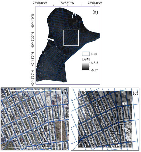
Figure 1 shows the study area, which is located in the northern part of Brooklyn, New York City, USA and includes large commercial and residential areas. The study area covers 6.12 km² land and contains approximately 8,000 buildings, 8,146 parcels, and 493 blocks. The elevation of the area ranges from −23 to 384 m. The land cover types in the area include buildings, vegetation, roads, bare soil, and oil tanks; the eastern and northern parts of the area are along the East River. Buildings in the area are complex in terms of size, texture, and shape.

Figure 1. Overview of the study area: (a) DSM; and (b) and (c) enlargements of the building areas in (a)

2.2 Data

The LiDAR point cloud data from the New York City Department of Information Technology and Telecommunications (NYCDITT 2019) covering the study area in 2017 were used to extract the building label information, 2D and 3D building morphological parameters, and landscape metrics. The data were collected using a Cessna 402 C or Cessna Caravan 208B aircraft equipped with Leica ALS80 and Riegl VQ-880-G laser systems from May 3 to 26 May 2017. The density of the point clouds is 8.0 points/m², and vegetated and non-vegetated vertical accuracy values are 15.8 and 6.4 cm, respectively, at the 95% confidence level (NYCDITT 2019). High-resolution orthophotos of red, green, blue, and near-infrared bands with a 0.3 m (1.0 ft) spatial resolution were collected from the New York City Office of Information Technology Services (NYITS 2019) as a reference to verify the extraction results.

3 Methodology

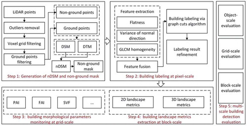
Figure 2 shows the workflow of the MS3DB method, which entails five key steps: (1) generation of normalized Digital Surface Model (nDSM) and non-ground mask; (2) building labeling at the pixel scale; (3) monitoring of 2D and 3D building morphological parameters; (4) extraction of 2D and 3D building landscape metrics; and (5) evaluation of multi-scale 3D building information.

Figure 2. Workflow of the proposed multi-scale 3D building information extraction method (MS3DB)

3.1 Generation of nDSM and non-ground points

The “StatisticalOutlierRemove” filter operation of PCL 1.6 was used for the point clouds to eliminate the noise in the data (Rusu et al. 2008). Then, the modified voxel grid filtering program (Du et al. 2017) was executed to reduce the excess points, where the size of the voxel was set to be slightly lower than the density of the original point clouds. The points nearest the voxel centroid were retained in each voxel to maintain the accuracy of the original point clouds.

The “lasground” filter operation of the LasTools (Rapidlasso 2020) was used to separate the noise-free point clouds into ground and non-ground points. Further, DSM and digital terrain model (DTM) data were produced using an interpolation algorithm (i.e., binning approach) with all points and ground points, respectively. The binning approach provides a cell assignment method to determine each output cell using the points that fall within its extent, along with a void fill method to determine the value of the cells that do not contain any LiDAR points (ESRI 2020). Here, the types of the cell assignment and void fill methods were set as the average and the natural neighbor, respectively (Dong and Chen 2018). Finally, nDSM was obtained by subtracting DTM data from DSM data. Besides, a non-ground mask of the point clouds with a height that was higher than zero was generated.

3.2 Building labeling at the object scale

3.2.1 Multi-feature extraction

Table 1 provides the details of the multi-feature extraction method developed in this study. Three features, flatness, variance of normal direction (Vnd), and GLCM homogeneity of nDSM, were selected for building labeling. Flatness was used because buildings often appear as plain surfaces, while vegetation can be considered to have an irregular surface. Vnd was used as another geometric feature because the normal vectors of vegetation are scattered and irregular in many directions, while those of buildings are fixed in a few directions. Lastly, in a height image, GLCM homogeneity of vegetation possesses a rich texture, while that of buildings has a simple texture.

Table 1. Multiple features used for building labeling

Feature	Calculation method	Reference
Flatness	$\{\text{ matrix{ {}{C}_{3*3}=\text{ {{{{}\sum \text{^ }^}\_}S\in N_S\left(S-\overline{S}\right){\left(S-\overline{S}\right)}^{\text{T}}\text{} over}\left|N_s\right|\text{}} cr}{F}_{fl}={\lambda }_0/\left({\lambda }_0+{\lambda }_1+{\lambda }_2\right)\text{ cr }}$where Ffl refers to the flatness of the non-ground point Si; NS is the set of nearest 15 non-ground points of point Si; C3*3 is a covariance matrix constructed from the set Ns;$\left|N_S\right|$$\left|N_S\right|$ refers to the number of points in the set NS; $\underset{-}{S}$$\underset{-}{S}$ is the central point of the set NS; ${\lambda }_0$${\lambda }_0$, ${\lambda }_1$${\lambda }_1$, and ${\lambda }_2$${\lambda }_2$ ($0\le {\lambda }_0\le {\lambda }_1\le {\lambda }_2$$0\le {\lambda }_0\le {\lambda }_1\le {\lambda }_2$) are the eigenvalues of C3*3.	Zhou and Neumann 2008; Lin et al. 2014
Variance of normal direction (Vnd)	$\left\{\begin{array}{c}{F}_{Vnd}=\frac{{\xi }^2}{u^2}\\ {\xi }^2=\frac{{\sum }_{i=1}^n\left(n_i-u\right)}{n}\\ u=\frac{\left|N_S\right|}{n}\end{array}\right.$$\left\{\begin{array}{c}{F}_{Vnd}=\frac{{\xi }^2}{u^2}\\ {\xi }^2=\frac{{\sum }_{i=1}^n\left(n_i-u\right)}{n}\\ u=\frac{\left|N_S\right|}{n}\end{array}\right.$where FVnd is the Vnd of the non-ground point Si; n is the number of direction bins, in this study, we set n = 6; ni refers to the number of points in the direction bin i; $\left|N_S\right|$$\left|N_S\right|$ is the number of points involved in the calculation; we choose the nearest 60 non-ground points of Si to participate in the calculation.	Du et al. 2017
GLCM homogeneity of nDSM	$\left\{\begin{array}{c}{F}_{th}=\sum _{i=1}^n\sum _{j=1}^n\frac{P\left(i,j,d,\theta \right)}{1+{\left(i-j\right)}^2}\\ P\left(i,j,d,\theta \right)=N_{gray\left(i,j\right)}withdand\theta \end{array}\right.$$\left\{\begin{array}{c}{F}_{th}=\sum _{i=1}^n\sum _{j=1}^n\frac{P\left(i,j,d,\theta \right)}{1+{\left(i-j\right)}^2}\\ P\left(i,j,d,\theta \right)=N_{gray\left(i,j\right)}withdand\theta \end{array}\right.$where Fth is the GLCM homogeneity of the nDSM; n refers to the gray level of the nDSM; i and j are the gray level of nDSM; d = 1 and $\theta =\left\{0^{\circ },{45}^{\circ },{90}^{\circ },and{135}^{\circ }\right\}$$\theta =\left\{0^{\circ },{45}^{\circ },{90}^{\circ },and{135}^{\circ }\right\}$ are the step size and direction of GLCM calculation, respectively; $P\left(i,j,d,\theta \right)$$P\left(i,j,d,\theta \right)$ is the joint conditional probability density; Ngray (i, j) reflects how many times the gray level pair (i, j) occur in a local slide window with given step size d, and direction θ; The sliding window size was set to 5 × 5 pixels; the final value of fth was the average value of four directions GLCM.	Haralick 1979; Liu et al. 2013

3.2.2 Feature fusion

The features have different value ranges; thus, the logistic function was used for normalization:

(1) $f\left(x\right)=\frac{1}{1+e^{-k\left(x-t_0\right)}},$$f\left(x\right)=\frac{1}{1+e^{-k\left(x-t_0\right)}},$(1)

where t₀ is the feature threshold, and its value greatly affects the labeling result (see Section 4.1 for the t₀ values for flatness, Vnd, and GLCM). k controls the steepness of the logistic function and has little effect on the labeling result. In this study, we set the values of k as −35.0, 2.0, and 0.2 for flatness, Vnd, and GLCM, respectively.

3.2.3 Graph-cut based building labeling

Because flatness, Vnd, and GLCM homogeneity describe the geometric characteristics of a pixel, they do not consider the consistency with surrounding pixels. Therefore, the extracted features were fused into a framework of minimum energy. We used the graph-cut algorithm (Boykov and Kolmogorov 2004) to perform the building labeling. The goal of the algorithm is to identify a label for each candidate pixel using the following energy function:

(2) $E\left(l\right)=\sum _{p\in P}{D}_p\left(l_p\right)+\beta \sum _{p,q\in N}{V}_{p,q}\left(l_p,l_q\right),$$E\left(l\right)=\sum _{p\in P}{D}_p\left(l_p\right)+\beta \sum _{p,q\in N}{V}_{p,q}\left(l_p,l_q\right),$(2)

where $\sum _{p\in P}{D}_p\left(l_p\right)$$\sum _{p\in P}{D}_p\left(l_p\right)$ represents the data cost, and $\sum _{p,q\in N}{V}_{p,q}\left(l_p,l_q\right)$$\sum _{p,q\in N}{V}_{p,q}\left(l_p,l_q\right)$ refers to the smoothness cost; D_p(l_p) is used to measure how well label l_p fits the node p; l_p refers to the building or non-building. D_p(l_p) can be calculated as follows:

(3) $\left\{\begin{array}{c}{D}_p\left(l_p=building\right)={\lambda }_{F\mathrm{\_}fl}\ast F_{fl}+\text{break}{\lambda }_{F\mathrm{\_}vnd}\ast F_{vnd}+{\lambda }_{F\mathrm{\_}th}\ast F_{th}\\ D_p\left(l_p=non-building\right)=1-\left({\lambda }_{F\mathrm{\_}fl}\ast F_{fl}\text{break}+{\lambda }_{F\mathrm{\_}vnd}\ast F_{vnd}+{\lambda }_{F\mathrm{\_}th}\ast F_{th}\right)\end{array},\right.$$\left\{\begin{array}{c}{D}_p\left(l_p=building\right)={\lambda }_{F\mathrm{\_}fl}\ast F_{fl}+\text{break}{\lambda }_{F\mathrm{\_}vnd}\ast F_{vnd}+{\lambda }_{F\mathrm{\_}th}\ast F_{th}\\ D_p\left(l_p=non-building\right)=1-\left({\lambda }_{F\mathrm{\_}fl}\ast F_{fl}\text{break}+{\lambda }_{F\mathrm{\_}vnd}\ast F_{vnd}+{\lambda }_{F\mathrm{\_}th}\ast F_{th}\right)\end{array},\right.$(3)

where F_fl, Fv_nd, and F_th are the normalized values of flatness, Vnd, and GLCM, respectively; ${\lambda }_{F\mathrm{\_}fl}$${\lambda }_{F\mathrm{\_}fl}$, ${\lambda }_{F\mathrm{\_}vnd}$${\lambda }_{F\mathrm{\_}vnd}$, and ${\lambda }_{F\mathrm{\_}th}$${\lambda }_{F\mathrm{\_}th}$ are the weights of flatness, Vnd, and GLCM, respectively (see Section 4.1 for more details).

The second term in Eq. (2)(2) $E\left(l\right)=\sum _{p\in P}{D}_p\left(l_p\right)+\beta \sum _{p,q\in N}{V}_{p,q}\left(l_p,l_q\right),$$E\left(l\right)=\sum _{p\in P}{D}_p\left(l_p\right)+\beta \sum _{p,q\in N}{V}_{p,q}\left(l_p,l_q\right),$(2) represents the degree of consistency between a node and its surrounding pixels. We used DSM to measure the consistency because the height difference of the building areas is small, whereas that between the areas of buildings and non-buildings is often large. The smoothness term can be calculated as follows:

(4) $V_{p,q}\left(l_p,l_q\right)=\frac{1}{{\left(h_p-h_q\right)}^2+{\epsilon }^2},$$V_{p,q}\left(l_p,l_q\right)=\frac{1}{{\left(h_p-h_q\right)}^2+{\epsilon }^2},$(4)

where h_p and h_q are the heights of pixels p and q. Constant ε was used to ensure that the denominator is greater than zero (Zarea and Mohammadzadeh 2016). Here, we set $\epsilon$$\epsilon$=0.2 m (Awrangjeb and Fraser 2014).

There is another parameter β in Eq. (2)(2) $E\left(l\right)=\sum _{p\in P}{D}_p\left(l_p\right)+\beta \sum _{p,q\in N}{V}_{p,q}\left(l_p,l_q\right),$$E\left(l\right)=\sum _{p\in P}{D}_p\left(l_p\right)+\beta \sum _{p,q\in N}{V}_{p,q}\left(l_p,l_q\right),$(2) . β is used to control the weight of the smooth term. It relates to the urban environment. If the buildings in the area are dense and tall, a high value of β is set. In this study, the study area was divided into 21 zones with a same size of 2500*2500 pixels (Figure 7). For accurate building labeling, the zones were set with various β values (see Table S1 for more details). In addition, we used zones 9 and 13 as experimental areas to determine t₀ values in Eq. (1)(1) $f\left(x\right)=\frac{1}{1+e^{-k\left(x-t_0\right)}},$$f\left(x\right)=\frac{1}{1+e^{-k\left(x-t_0\right)}},$(1) for flatness, Vnd, and GLCM because buildings in these two zones represent typical tall and small ones, respectively. The graph-cut algorithm was employed to examine the influence of t₀ on a feature.

3.2.4 Labeling refinement

Figure 3 shows the procedure for building labeling refinement. First, the height and area thresholds were used to remove irrelevant low buildings and small building patches, respectively (see Table S1 for details).

Figure 3. Procedure for labeling refinement

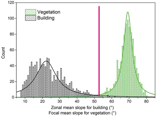
In addition, a zonal slope threshold was applied to remove small vegetation patches. The zonal mean slope threshold was determined by the difference in the slope histogram between vegetation and buildings (Figure 4). 1000 building footprints and 1000 medium/high vegetation points were randomly selected to determine their zonal mean slope values and focal mean slopes. A mask of 21 × 21 pixels (10.5 m × 10.5 m) was used to calculate the value of the focal mean slope. The maximum value of the zonal mean slope of buildings was selected as the threshold. As shown in Figure 4, the zonal mean slope threshold was set to 53° to identify and remove small vegetation patches.

Finally, because some holes existed on building surfaces after labeling, a morphological opening operation followed by a closing operation was used to refine the labeling results. The kernel for opening and closing operations was set to the 3 × 3 window size. In this way, an accurate building footprint can be obtained and subsequently used in the extraction of parameters and landscape metrics.

Figure 4. Zonal mean slope threshold for separating buildings and vegetation

3.3 Extraction of building morphological parameters at the grid scale

There is a trade-off between the accuracy and detail loss of extracted parameters (Susaki, Kajimoto, and Kishimoto 2014; Huang et al. 2017). As the size of a grid increases, the accuracy of extracted parameters gradually increases but the details are lost. However, when the size of a grid is sufficiently large, the accuracy of the extracted parameters becomes stable (Susaki, Kajimoto, and Kishimoto 2014). The Pearson coefficient between morphological parameters extracted from the labeling and ground truth building data was computed to measure the changes in accuracy at different sizes of a grid. The Kullback-Leibler (KL) value was calculated to assess the differences in the details of extracted parameters at various grid sizes:

(5) $KL(P||Q)=\sum _{i}P\left(i\right)log\frac{P\left(i\right)}{Q\left(i\right)},$$KL(P||Q)=\sum _{i}P\left(i\right)log\frac{P\left(i\right)}{Q\left(i\right)},$(5)

where KL (P||Q) denotes the KL value, and P and Q refer to the discrete probability distributions of the ground truth building density with refined spatial resolution and the extracted building density with coarse spatial resolution, respectively. Various grid sizes were considered, 7 × 7, 11 × 11, 21 × 21, 31 × 31, 41 × 41, and 51 × 51 pixels. The distributions of urban density [0%, 100%] with an interval of 1% at different grid sizes were compared to those at the 7 × 7 pixels. Table 2 shows the 2D and 3D building morphological parameters as well as the calculation method used in this study. Parameters listed in Table 2 were selected for grid-scale monitoring.

Table 2. Building 2D/3D morphological parameters used in this study

Parameter	Abbreviation	Formula or calculation method	Reference
Area	A	$\mathrm{A}=A_{building}$$\mathrm{A}=A_{building}$	Yu et al. 2010
Volume	V	$\mathrm{V}=V_{building}$$\mathrm{V}=V_{building}$	Yu et al. 2010
Planar Area Index	PAI	$\mathrm{P}\mathrm{A}\mathrm{I}=\frac{A_{building}}{A_{grid}}$$\mathrm{P}\mathrm{A}\mathrm{I}=\frac{A_{building}}{A_{grid}}$	Kanda, Kawai, and Nakagawa 2005a
Frontal Area Index	FAI	$\mathrm{F}\mathrm{A}\mathrm{I}=\frac{A_{fa}}{A_{grid}}$$\mathrm{F}\mathrm{A}\mathrm{I}=\frac{A_{fa}}{A_{grid}}$	Kanda, Kawai, and Nakagawa 2005a
Ratio of Street Height and Building Width	H/W	$\mathrm{H}/\mathrm{W}=\frac{H_{building}}{W_{building}}$$\mathrm{H}/\mathrm{W}=\frac{H_{building}}{W_{building}}$	Kanda et al. 2005b
Ratio of Street Height and Width	H/L	$\mathrm{H}/\mathrm{L}=\frac{H_{building}}{L_{road}}$$\mathrm{H}/\mathrm{L}=\frac{H_{building}}{L_{road}}$	Kanda et al. 2005b
Sky View Factor of Rooftop or Ground	RGSVF	$\mathrm{R}\mathrm{G}\mathrm{\_}\mathrm{S}\mathrm{V}\mathrm{F}=1-\frac{{\sum }_{i=1}^{n}sin{\gamma }_i}{n}$$\mathrm{R}\mathrm{G}\mathrm{\_}\mathrm{S}\mathrm{V}\mathrm{F}=1-\frac{{\sum }_{i=1}^{n}sin{\gamma }_i}{n}$	Zakšek, Oštir, and Kokalj 2011
Sky View Factor of Vertical Wall	WSVF	$\mathrm{W}\mathrm{\_}\mathrm{S}\mathrm{V}\mathrm{F}=\mathrm{F}\mathrm{\_}\mathrm{W}\mathrm{V}\mathrm{F}\ast \left(1-PAI\right)\ast FAI$$\mathrm{W}\mathrm{\_}\mathrm{S}\mathrm{V}\mathrm{F}=\mathrm{F}\mathrm{\_}\mathrm{W}\mathrm{V}\mathrm{F}\ast \left(1-PAI\right)\ast FAI$	Yang et al. 2015

A_grid is the area of a grid; A_fa is frontal area of a grid; H_building and W_building are building height and width; L_road is building length; n refers to the direction number of calculated sky view factor; and γ_i stands for the elevation angle of the relief horizon in calculated direction i.

3.4 Extraction of building landscape metrics at the city-block level

Table 3 shows the 2D and 3D landscape metrics used in this study. The 2D landscape metrics included building area coverage (BAC) and the mean building area (MBA). A set of 3D building landscape metrics for the city block, such as high building ratio (HBR), mean building height (MBH), mean building structure index (MBSI), and floor area ratio (FAR), were integrated. Note that following Craighead (2009), in the United States, high buildings are defined as those with a height ≥ 22.5 m.

Table 3. Building landscape metrics at the block-scale

Category	Landscape metric	Abbreviation	Formula	Definition
2D landscape metric	Building area coverage	BAC	$\mathrm{B}\mathrm{A}\mathrm{C}=\frac{{\sum }_{i=1}^N{A}_{buildingi}}{A_{block}}$$\mathrm{B}\mathrm{A}\mathrm{C}=\frac{{\sum }_{i=1}^N{A}_{buildingi}}{A_{block}}$	Sum of building area divided by block area.
	Mean building area	MBA	$\mathrm{M}\mathrm{B}\mathrm{A}=\frac{{\sum }_{i=1}^N{A}_{buildingi}}{N}$$\mathrm{M}\mathrm{B}\mathrm{A}=\frac{{\sum }_{i=1}^N{A}_{buildingi}}{N}$	Average building area in a block.
	Standard deviation of building area	SDBA	$\mathrm{S}\mathrm{D}\mathrm{B}\mathrm{A}=\sqrt{\frac{{\sum }_{i=1}^N{\left(A_{buildingi}-MBA\right)}^2}{N}}$$\mathrm{S}\mathrm{D}\mathrm{B}\mathrm{A}=\sqrt{\frac{{\sum }_{i=1}^N{\left(A_{buildingi}-MBA\right)}^2}{N}}$	Standard deviation of building area in a block.
	Largest patch index	LPI	$\mathrm{L}\mathrm{P}\mathrm{I}=\frac{A_{max}}{{\sum }_{i=1}^N{A}_{buildingi}}$$\mathrm{L}\mathrm{P}\mathrm{I}=\frac{A_{max}}{{\sum }_{i=1}^N{A}_{buildingi}}$	Largest building area divided by sum of building area.
	Mean nearest neighbor distance	MNN	$\mathrm{M}\mathrm{N}\mathrm{N}=\frac{{\sum }_{i=1}^N{d}_{ni}}{N}$$\mathrm{M}\mathrm{N}\mathrm{N}=\frac{{\sum }_{i=1}^N{d}_{ni}}{N}$	Average nearest distance to a neighbor for building patches in a block.
3D landscape metric	High building ratio	HBR	$\mathrm{H}\mathrm{B}\mathrm{R}=\frac{N_h}{N}$$\mathrm{H}\mathrm{B}\mathrm{R}=\frac{N_h}{N}$	Number of buildings higher than 22.5 m divided by total building number in a block.
	Mean building height	MBH	$\mathrm{M}\mathrm{B}\mathrm{H}=\frac{{\sum }_{i=1}^N{h}_{buildingi}}{N}$$\mathrm{M}\mathrm{B}\mathrm{H}=\frac{{\sum }_{i=1}^N{h}_{buildingi}}{N}$	Average building height in a block.
	Area-weighted mean building height	AMBH	$\mathrm{A}\mathrm{M}\mathrm{B}\mathrm{H}=\sum _{i=1}^N{f}_i\ast h_{buildingi}$$\mathrm{A}\mathrm{M}\mathrm{B}\mathrm{H}=\sum _{i=1}^N{f}_i\ast h_{buildingi}$	Average building height balanced by area in a block.
	Height deviation among buildings	HDB	$\mathrm{H}\mathrm{D}\mathrm{B}=\sqrt{\frac{{\sum }_{i=1}^N{\left(h_{buildingi}-MBH\right)}^2}{N}}$$\mathrm{H}\mathrm{D}\mathrm{B}=\sqrt{\frac{{\sum }_{i=1}^N{\left(h_{buildingi}-MBH\right)}^2}{N}}$	Height variation of buildings in a block.
	Mean building structure index	MBSI	$\mathrm{M}\mathrm{B}\mathrm{S}\mathrm{I}=\frac{1}{N}\ast \sum _{i=1}^N\frac{A_{buildingi}}{h_{buildingi}}$$\mathrm{M}\mathrm{B}\mathrm{S}\mathrm{I}=\frac{1}{N}\ast \sum _{i=1}^N\frac{A_{buildingi}}{h_{buildingi}}$	Average value of ratio of building area and height in a block.
	Floor area ratio	FAR	$\mathrm{F}\mathrm{A}\mathrm{R}=\frac{{\sum }_{i=1}^N{c}_i\ast F_i}{A_{block}}$$\mathrm{F}\mathrm{A}\mathrm{R}=\frac{{\sum }_{i=1}^N{c}_i\ast F_i}{A_{block}}$	Total building floor area divided by block area.

h_buildingi and A_buildingi are the area of building i, respectively; N represents building number in a block; A_block is the area of a city block; A_max is the area of the largest building in a block; and d_ni is the nearest distance of building i to a neighbor of a building patch; f_i is the proportion of building i area; and c_i and F_i refer to floor number and area within building i.

3.5 Evaluation of multi-scale extraction of buildings

3.5.1 Object scale evaluation

Pixel-based, object-based, and area-normalized object-based methods were used to assess the accuracy of building labeling at the object scale.

(1) Pixel-based method

A true positive (TP) pixel is a pixel labeled as “building” that corresponds to the “building” in the reference; a false negative (FN) pixel corresponds to the building that is labeled as “non-building” in the reference; a false positive (FP) pixel is labeled as “building” that corresponds to “non-building” in the reference (Rutzinger, Rottensteiner, and Pfeifer 2009). Based on these definitions, three metrics were defined to evaluate the accuracy of the results: completeness (Comp), correctness (Corr), and Quality.

(6) $\left\{\begin{array}{c}Com{p}_{area}=\frac{{\sum }_{i=1}^{N_{tpcomp}}Area\mathrm{\_}tpcom{p}_i}{{\sum }_{i=1}^{N_{tpcomp}}Area\mathrm{\_}tpcom{p}_i+{\sum }_{i=1}^{N_{fn}}Area\mathrm{\_}f{n}_i}\\ Cor{r}_{area}=\frac{{\sum }_{i=1}^{N_{tpcorr}}Area\mathrm{\_}tpcor{r}_i}{{\sum }_{i=1}^{N_{tpcorr}}Area\mathrm{\_}tpcor{r}_i+{\sum }_{i=1}^{N_{fp}}Area\mathrm{\_}f{p}_i}\\ Qualit{y}_{area}=\frac{Com{p}_{area}\ast Cor{r}_{area}}{Com{p}_{area}+Cor{r}_{area}+Com{p}_{area}\ast Cor{r}_{area}}\end{array}\right.,$$\left\{\begin{array}{c}Com{p}_{area}=\frac{{\sum }_{i=1}^{N_{tpcomp}}Area\mathrm{\_}tpcom{p}_i}{{\sum }_{i=1}^{N_{tpcomp}}Area\mathrm{\_}tpcom{p}_i+{\sum }_{i=1}^{N_{fn}}Area\mathrm{\_}f{n}_i}\\ Cor{r}_{area}=\frac{{\sum }_{i=1}^{N_{tpcorr}}Area\mathrm{\_}tpcor{r}_i}{{\sum }_{i=1}^{N_{tpcorr}}Area\mathrm{\_}tpcor{r}_i+{\sum }_{i=1}^{N_{fp}}Area\mathrm{\_}f{p}_i}\\ Qualit{y}_{area}=\frac{Com{p}_{area}\ast Cor{r}_{area}}{Com{p}_{area}+Cor{r}_{area}+Com{p}_{area}\ast Cor{r}_{area}}\end{array}\right.,$(6)

where N_TP represents the number of TP pixels; N_FN represents the number of FN pixels; and N_FP represents the number of FP pixels.

(2) Object-based method

For each detected building, the percentage of the area of the detected building that overlaps with the reference label image is evaluated. A percent threshold of 70% was selected to classify each detected building either as a TP_corr or FP (Rutzinger, Rottensteiner, and Pfeifer 2009). Similarly, for each building in the reference, the percentage of the area of the building in the reference that overlaps with the detected label image was calculated. The percent thresholds were compared to classify each building in the reference either as TP_comp or FN.

(3) Area-normalized object-based method

Besides pixel-based and object-based methods, an area-normalized object-based method was also employed for more accurate and comprehensive accuracy assessment:

(7) $\left\{\begin{array}{c}Com{p}_{area}=\frac{{\sum }_{i=1}^{N_{tpcomp}}Area\mathrm{\_}tpcom{p}_i}{{\sum }_{i=1}^{N_{tpcomp}}Area\mathrm{\_}tpcom{p}_i+{\sum }_{i=1}^{N_{fn}}Area\mathrm{\_}f{n}_i}\\ Cor{r}_{area}=\frac{{\sum }_{i=1}^{N_{tpcorr}}Area\mathrm{\_}tpcor{r}_i}{{\sum }_{i=1}^{N_{tpcorr}}Area\mathrm{\_}tpcor{r}_i+{\sum }_{i=1}^{N_{fp}}Area\mathrm{\_}f{p}_i}\\ Qualit{y}_{area}=\frac{Com{p}_{area}\ast Cor{r}_{area}}{Com{p}_{area}+Cor{r}_{area}+Com{p}_{area}\ast Cor{r}_{area}}\end{array}\right.,$$\left\{\begin{array}{c}Com{p}_{area}=\frac{{\sum }_{i=1}^{N_{tpcomp}}Area\mathrm{\_}tpcom{p}_i}{{\sum }_{i=1}^{N_{tpcomp}}Area\mathrm{\_}tpcom{p}_i+{\sum }_{i=1}^{N_{fn}}Area\mathrm{\_}f{n}_i}\\ Cor{r}_{area}=\frac{{\sum }_{i=1}^{N_{tpcorr}}Area\mathrm{\_}tpcor{r}_i}{{\sum }_{i=1}^{N_{tpcorr}}Area\mathrm{\_}tpcor{r}_i+{\sum }_{i=1}^{N_{fp}}Area\mathrm{\_}f{p}_i}\\ Qualit{y}_{area}=\frac{Com{p}_{area}\ast Cor{r}_{area}}{Com{p}_{area}+Cor{r}_{area}+Com{p}_{area}\ast Cor{r}_{area}}\end{array}\right.,$(7)

where Comp_area, Corr_area, and Quality_area are the completeness, correctness, and quality metrics calculated via the object-based method normalized by area; N_tpcomp and N_fn are the number of TP_comp and FN buildings; Area_tpcomp_i is the area of TP_comp building i; Area_fn_i is the area of FN building i; N_tpcorr and N_fp are the number of TP_corr and FP buildings; Area_tpcorr_i is the area of TP_corr building i; and Area_fp_i is the area of FP building i.

3.5.2 Grid- and block-scale evaluation

Grid- and block-scale results were compared with the visualization results. The Pearson correlation coefficient and parameters of the regression equation in Eq. (8)(8) $y=ax+b,$$y=ax+b,$(8) were used to evaluate the grid- and block-scale results.

(8) $y=ax+b,$$y=ax+b,$(8)

where x and y refer to the parameters/landscape metrics extracted from the MS3DB method and those extracted from the visualization results; a and b are the regression coefficients. Higher correlation coefficients (R²) associated with a values closer to one and b values closer to zero in the regression equation indicate greater similarity between parameters/landscape metrics extracted from the MS3DB method and those extracted from visualization results.

4. Results

4.1 Determination of parameters

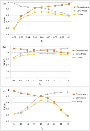
Several key parameters in this study can affect the accuracy of the MS3DB method. For example, parameter t₀ in Eq. (1)(1) $f\left(x\right)=\frac{1}{1+e^{-k\left(x-t_0\right)}},$$f\left(x\right)=\frac{1}{1+e^{-k\left(x-t_0\right)}},$(1) greatly affects the labeling results. Figure 5 shows the effect of t₀ on flatness, Vnd, and GLCM of the labeling results. Comp, Corr, and Quality of the labeling results using the pixel-based evaluation method for different t₀ values were acquired. We selected the highest Quality to determine the optimal t₀ value. The highest values of Quality for flatness, Vnd, and GLCM were determined when t₀ was 0.06, 0.80, and 18.00, respectively.

Figure 5. Parameter t₀ analysis: (a) t₀ on flatness; (b) t₀ on Vnd; and (c) t₀ on GLCM

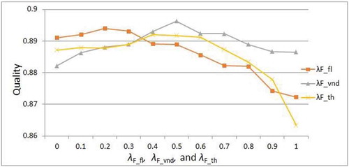
In addition to t₀, other parameters, λ_{F_fl}, λ_{F_vnd}, and λ_{F_th} in Eq. (3)(3) $\left\{\begin{array}{c}{D}_p\left(l_p=building\right)={\lambda }_{F\mathrm{\_}fl}\ast F_{fl}+\text{break}{\lambda }_{F\mathrm{\_}vnd}\ast F_{vnd}+{\lambda }_{F\mathrm{\_}th}\ast F_{th}\\ D_p\left(l_p=non-building\right)=1-\left({\lambda }_{F\mathrm{\_}fl}\ast F_{fl}\text{break}+{\lambda }_{F\mathrm{\_}vnd}\ast F_{vnd}+{\lambda }_{F\mathrm{\_}th}\ast F_{th}\right)\end{array},\right.$$\left\{\begin{array}{c}{D}_p\left(l_p=building\right)={\lambda }_{F\mathrm{\_}fl}\ast F_{fl}+\text{break}{\lambda }_{F\mathrm{\_}vnd}\ast F_{vnd}+{\lambda }_{F\mathrm{\_}th}\ast F_{th}\\ D_p\left(l_p=non-building\right)=1-\left({\lambda }_{F\mathrm{\_}fl}\ast F_{fl}\text{break}+{\lambda }_{F\mathrm{\_}vnd}\ast F_{vnd}+{\lambda }_{F\mathrm{\_}th}\ast F_{th}\right)\end{array},\right.$(3) also affect the labeling results. λ_{F_fl}, λ_{F_vnd}, and λ_{F_th} refer to the weight of F_fl, F_vnd, and F_th, respectively. Since zones 9 and 13 were selected as the experimental areas, we calculated Quality values of the pixel-based evaluation method to analyze the effect of these weighting parameters on the labeling results. The values of λ_{F_fl}, λ_{F_vnd}, and λ_{F_th} were normalized from 0.1 to 1.0 at the interval of 0.1. When one weight value was a, the other two values were calculated as (1-a)/2 to ensure that their sum is equal to 1. Figure 6 shows the parameter analysis of λ_{F_fl}, λ_{F_vnd}, and λ_{F_th}. The highest Quality value was obtained when λ_{F_vnd} = 0.5. Therefore, we set λ_{F_fl}, λ_{F_vnd}, and λ_{F_th} as 0.25, 0.50, and 0.25, respectively.

Figure 6. Parameter analysis of λ_{F_fl}, λ_{F_vnd}, and λ_{F_th.}

4.2 Building labeling at the object scale

Table 4 shows the evaluation of the building labeling methods. Results of the pixel-based, object-based, and area-normalized object-based evaluation methods for 21 zones were consistent. Comp, Corr, and Quality in the entire area were 94.49%, 95.54%, and 90.51%; 94.21%, 97.99%, and 92.42%; and 98.38%, 99.41%, and 97.81% using pixel-based evaluation, object-based evaluation, and area-normalized object-based, respectively. These results suggest that the MS3DB method achieved a reasonable accuracy for large-area buildings. All the experiments confirm the feasibility of the methods.

Table 4. Accuracy of building labeling

ID	Pixel-based evaluation (%)			Object-based evaluation (%)			Area-normalized object-based evaluation (%)
	Comp	Corr	Quality	Comp	Corr	Quality	Comp	Corr	Quality
1	95.19	97.06	95.52	92.51	92.91	86.41	98.99	98.84	97.85
2	96.93	97.56	94.63	88.00	86.95	77.73	99.97	99.21	99.18
3	95.04	93.67	89.31	100.00	100.00	100.00	100.00	100.00	100.00
4	92.71	97.00	90.13	94.83	98.89	93.83	97.43	99.37	96.83
5	95.05	96.44	91.83	87.59	92.66	81.91	98.41	98.97	97.41
6	91.67	97.59	89.65	76.67	91.00	71.27	96.32	98.30	94.47
7	99.60	95.92	95.55	100.00	100.00	100.00	100.00	100.00	100.00
8	93.98	97.51	91.78	93.01	98.75	91.93	98.41	99.62	98.04
9	93.11	97.26	90.73	94.11	99.62	93.77	97.80	99.87	97.68
10	94.93	98.18	93.30	96.96	98.25	95.31	99.41	99.41	98.83
11	96.49	98.29	94.40	90.47	82.61	76.00	99.51	99.41	98.93
12	93.99	96.38	90.79	86.34	97.83	84.72	98.94	99.42	98.37
13	96.41	92.04	88.99	94.93	96.09	91.40	98.58	98.76	97.38
14	93.45	96.17	90.10	95.36	99.18	94.61	98.95	99.43	98.39
15	97.40	92.70	90.46	92.53	96.82	90.46	97.41	98.47	95.96
16	92.67	95.12	88.46	92.80	97.71	90.82	97.03	99.54	96.60
17	97.93	90.20	88.51	96.43	98.23	94.78	99.30	99.64	98.95
18	96.00	94.06	90.51	95.05	98.93	94.08	99.37	99.92	99.29
19	94.71	94.42	89.56	96.30	96.85	93.38	99.64	99.55	99.19
20	92.24	94.10	87.19	94.21	98.68	93.04	96.28	99.32	95.65
21	92.30	95.81	88.72	98.43	100.00	98.43	99.20	100.00	99.20
Average	94.49	95.54	90.51	94.21	97.99	92.42	98.38	99.41	97.81

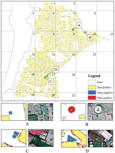
Figure 7 shows the refined labeling results extracted from the MS3DB method at the pixel scale. Wrong labeling was detected in three situations: (1) some small buildings were missing, (2) some oil tanks were wrongly labeled as buildings, and (3) some buildings were wrongly labeled as non-buildings due to the influence of vegetation on some rooftops. These errors are expected because a single LiDAR data source can only obtain the height information of urban features. It can be challenge to distinguish oil tanks from buildings and to identify vegetations on rooftops.

Figure 7. Extracted buildings using the pixel-based evaluation method and classification errors (missing small buildings, confusing buildings with oil tanks)

4.3 Extraction of morphological parameters at the grid scale

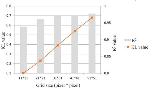
The spatial resolution of the building labeling results was set as 0.5 m × 0.5 m. For 2D and 3D building morphological parameters at the grid scale, the grid size should be determined by fully considering the accuracy and loss of detail. Figure 8 shows the effect of different grid sizes on the extracted results. The R² value became stable at the grid size of 31 × 31 pixels, while the KL value still increased at that size. A smaller KL value indicates that the urban density distribution of the size is more similar to that of 7 × 7 pixels. Therefore, considering the trade-off between accuracy and loss of detail, we selected 31 × 31 pixels as the final grid size.

Figure 8. Comparison between the extraction accuracy (R²) and loss of detail (KL value) at different grid sizes

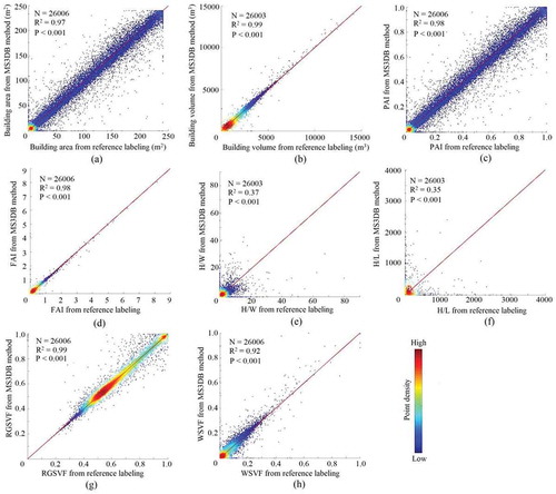
Figure 9 shows the extraction of the grid-scale parameters using the MS3DB method, e.g., area, volume, PAI, and FAI (see Table 2 for definitions). Figure 10 shows the scatter plots of the 2D and 3D building morphological parameters against those from the visual interpretation, which include building area, volume, PAI, FAI, RGSVF, and WSVF (see Table 2 for definitions). Most parameters yielded R² values greater than 0.92, except for H/W and H/L, which had R² values of 0.37 and 0.35, respectively. These results imply that the MS3DB method extracted the building edges with limited accuracy because of the “salt and pepper” noise in the grid-scale results.

Figure 9. Extraction results of grid-scale building parameters: (a)–(g) refer to the area, volume, Planer area index (PAI), Frontal Area Index (FAI), ratio of street height and building width (H/W), ratio of street height and width (H/L), sky view factor of rooftop or ground (RGSVF), and sky view factor of vertical wall (WSVF), respectively

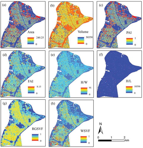
Figure 10. Scatter plots of building morphological parameters against those from reference labeling: (a)–(g) refer to area, volume, PAI, FAI, H/W, H/L, RGSVF, and WSVF, respectively; red line means 1:1 (i.e. slope = 1 and intercept = 0) line

4.4 Extraction of building landscape metrics at the block scale

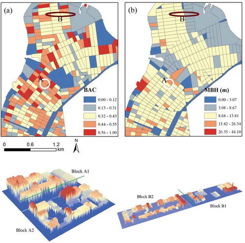
Figure 11 shows the block-scale results of BAC and MBH. BAC refers to the ratio of the total building area and the block area, whereas MBH refers to the average height of the block. The natural breakpoint method was used to divide the landscape metrics into five categories (Smith 1986). Blocks at locations A and B shared the same BAC; however, large differences in their MBH were observed. Such differences in the vertical landscape at the block-scale were detected using the MS3DB method. This shows the benefits of integrating 2D and 3D landscapes for a better understanding of the structure of urban buildings.

Figure 11. Block-scale building landscape metrics: (a) building area coverage (BAC); and (b) mean building height (MBH)

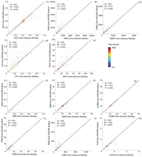
Figure 12 demonstrates the comparison of the results of the landscape metrics extracted using the MS3DB method and those extracted by visual interpretation. The results in Figure 12 imply that overall, refined extraction accuracy was achieved for most metrics. AMBH showed the highest accuracy with R² of 0.97. The accuracy for MBSI and LPI was lower than for the other metrics with R² values of 0.62 and 0.67.

Figure 12. Scatter plots of 2D and 3D landscape metrics from the MS3DB method against those from the reference labeling: (a)–(k) refer to BAC, MBA, SDBA, LPI, MNN, HBR, MBH, AMBH, HDB, MBSI, and FAR, respectively; red line means 1:1 (i.e. slope = 1 and intercept = 0) line

5 Discussion

In this study, a new 3D building detection method (MS3DB) was developed at the pixel, grid, and block scales using both morphological parameters and landscape metrics. The new method is a useful tool for city managers to solve urban problems because it ensures GIS data accuracy and reliability for urban analysis at different spatial scales and thus optimizes urban planning costs. This method can also provide support for urban climate and energy studies because 2D/3D building morphological parameters and landscape patterns are important variables in urban climate and energy budget models (Kanda, Kawai, and Nakagawa 2005a; Yang et al. 2015; Zheng and Weng 2019).

We further evaluated the performance of the proposed method by using the point clouds data from Areas 1–3 of the ISPRS Test Project on Urban Classification and 3D Building Reconstruction (Rottensteiner et al. 2014). In this way, our method can be compared with existing methods by using the same data from the ISPRS benchmark dataset. Table 5 presents the comparison of the MS3DB method with the existing methods in terms of accuracy, data sources, verification method, and spatial scale. The advantages of the MS3DB method can be summarized as follows. First, the MS3DB method produces more accurate results than most existing methods using a single LiDAR data source. Larger-area buildings (area >50 m²) yield high accuracy in the MS3DB method. The Comp, Corr, and Quality values of the object-based method were 100%, indicating no false extraction of the building objects.

Table 5. Comparison between existing methods and the MS3DB method

Method	Data source	Verify method	Outputs	Object-based evaluation (%)			Object-based>50 m^2 evaluation (%)
				Comp	Corr	Quality	Comp	Corr	Quality
Threshold-based segmentation (Yu et al. 2010)	Airborne LiDAR and color near-infrared image	Only building object	Building object and 2D/3D morphological parameter	-	-	-	-	-	-
Urban analysis approach (Diego et al., 2013)	Airborne LiDAR	Only building object	Building geometric information and density attributes	-	-	-	-	-	-
WHUY1 (Yang, Xu, and Dong 2013)	Airborne LiDAR	Pixel and object	Building footprint	77.6	98.1	76.5	97.4	97.9	95.4
UMTA (Feng 2020)	Airborne LiDAR	Pixel and object	Building footprint	80.0	98.6	79.1	99.1	100.0	99.1
MON (Awrangjeb and Fraser 2014)	Airborne LiDAR	Pixel and object	Building footprint	80.0	98.6	79.1	99.1	100.0	99.1
WHU_QC (Chen and Sun 2020)	Airborne LiDAR	Pixel and object	Building footprint	80.9	99.0	80.3	96.8	100.0	96.8
MON4 (Siddiqui et al. 2020)	Airborne LiDAR	Pixel and object	Building footprint	83.9	93.8	79.3	99.1	100.0	99.1
WHU_YD (Yang 2020)	Airborne LiDAR	Pixel and object	Building footprint	87.8	99.3	87.3	99.1	100.0	99.1
MS3DB	Airborne LiDAR	Pixel, object, grid, and block	Building footprint, 2D/3D morphological parameter, and landscape metrics	84	100	84	100	100	100

Second, the accuracy of the extraction of the 3D building information was evaluated at the pixel, object, grid, and block-scales. This information is essential for urban managers, planners, and urban data users because urban building analysis is often conducted at different spatial scales.

Third, several 3D building landscape metrics were integrated into MS3DB for block-scale detection. By adding height information extracted from the LiDAR data, 2D landscape metrics can be further improved (Figure 11). It is of practical importance for urban planners to perform urban analysis at the city-block level because city blocks are often the basic urban management units.

This study has several limitations. First, this study focuses on 3D building information detection; however, more urban elements are required to perform multi-scale urban analysis, e.g., tree object identification and canopy height evaluation. Second, the use of a single LiDAR data source generated some errors in the labeling results (Figure 7), e.g., missing small buildings and confusing buildings with oil tanks. Thus, future research should focus on the detection of additional urban features and synthesizing multi-source remote sensing data (e.g., VHR data) to take advantage of multi-modal data for more accurate building labeling.

6 Conclusions

In this study, a method of multi-scale 3D building information extraction (MS3DB) was developed for urban areas using a single LiDAR point cloud and tested in the northern part of Brooklyn, New York City, USA. The method effectively extracted accurate building labeling information at the object scale, building 2D and 3D morphological parameters at the grid scale, and 3D building landscape metrics at the city-block scale. Several accuracy evaluation methods were integrated into the MS3DB method at the object, grid, and block scales. The findings of this study contribute to the existing knowledge on the extraction of multi-scale 3D building information. The major results of the study can be summarized as follows:

The extraction accuracy of building labeling over the entire study area was highly consistent. The Comp, Corr, and Quality metrics of the object-based evaluation method were 94.21%, 97.99%, and 92.42%, respectively. Most of the grid-scale parameters, i.e., building area, volume, PAI, FAI, RGSVF, and WSVF, achieved high extraction accuracy with R² > 0.92, except for H/W and H/L, with R² of 0.37 and 0.35, respectively. This indicates that the MS3DB method did not extract building edges successfully. For the block-scale extraction of the landscape metrics, AMBH achieved the highest accuracy (R² = 0.97), while the accuracy of MBSI and LPI was lower than the other metrics (R² = 0.62 and 0.67, respectively).

The main contributions of this study can be summarized as follows. First, it successfully combines the building objects, 2D/3D morphological parameters, and landscape metrics in a holistic detection method, which is rarely reported in the literature. Second, various evaluation methods of building extraction at the object, grid, and block scale were designed in the MS3DB. This is useful for determining the reliability of the results at different spatial scales. Finally, the proposed MS3DB method can extract both 2D and 3D landscape metrics, instead of the traditional methods that extract only 2D landscape metrics.

Highlights

• Multi-scale 3D building information extraction (MS3DB) method was proposed.

• MS3DB extracts building labels, 2D/3D morphological parameters, & landscape metrics.

• 3D building landscape metrics was integrated into MS3DB for block-scale detection.

• Accuracy of MS3DB at object-, grid-, and block-scale was evaluated.

Acknowledgements

The authors would like to thank the editors and anonymous reviewers for their valuable time and efforts in reviewing this manuscript and the New York City Department of Information Technology and Telecommunications for their efforts to make the ALS data free to download.

Data availability statement

Data in this study can be available within the article or its supplementary materials. 2017 ALS data used in this study can be download from http://gis.ny.gov/elevation/lidar-coverage.htm.

Disclosure statement

No potential conflict of interest was reported by the authors.

Additional information

Funding

This research was supported by the National Natural Science Foundation (NSFC) of China [Key Project #41930650], and funded by Beijing Key Laboratory of Urban Spatial Information Engineering [No. 2020210].

References

- Adolphe, L. 2001. “A Simplified Model of Urban Morphology: Application to an Analysis of the Environmental Performance of Cities.” Environment and Planning B: 28 (2): 183–200. doi:10.1068/b2631.
- Awrangjeb, M., and C. S. Fraser. 2014. “Automatic Segmentation of Raw LiDAR Data for Extraction of Building Roofs.” Remote Sensing 6 (5): 3716–3751. doi:10.3390/rs6053716.
- Baltsavias, E. P. 1999. “A Comparison between Photogrammetry and Laser Scanning.” ISPRS Journal of Photogrammetry and Remote Sensing 54: 83–94. doi:10.1016/s0924-2716(99)00014-3.
- Bouziani, M., K. GoTa, and D. C. He. 2010. “Automatic Change Detection of Buildings in Urban Environment from Very High Spatial Resolution Images Using Existing Geodatabase and Prior Knowledge.” ISPRS Journal of Photogrammetry and Remote Sensing 65 (1): 143–153. doi:10.1016/j.isprsjprs.2009.10.002.
- Boykov, Y., and V. Kolmogorov. 2004. “An Experimental Comparison of Min-cut/maxflow Algorithms for Energy Minimization in Vision.” IEEE Transactions on Pattern Analysis and Machine Intelligence 26 (9): 1124–1137. doi:10.1109/tpami.2004.60.
- Cao, S., M. Du, W. Zhao, Y. Hu, Y. Mo, S. Chen, Y. Cai, Z. Peng, and C. Zhang. 2020. “Multi-level Monitoring of Three-dimensional Building Changes for Megacities: Trajectory, Morphology, and Landscape.” ISPRS Journal of Photogrammetry and Remote Sensing 167 (2020): 54–70. doi:10.1016/j.isprsjprs.2020.06.020.
- Chen, Q., and M. Sun 2020. “Brief Description of Building Detection from Airborne LiDAR Data Based on Extraction of Planar Structure.” Accessed 1 March 2020. http://ftp.ipi.uni-hannover.de/ISPRS_WGIII_website/ISPRSIII_4_Test_results/papers/Brief_description_Qi_Chen_WHU.pdf
- Chen, Z., B. Xu, and B. Devereux. 2019. “Urban Landscape Pattern Analysis Based on 3d Landscape Models.” Applied Geography 55: 82–91. doi:10.1016/j.apgeog.2014.09.006.
- Craighead, G. 2009. Chapter 1 – High-Rise Building Definition, Development, and Use in Book High-Rise Security and Fire Life Safety. Oxford, UK: Elsevier’s Science & Technology Rights Department.
- Deng, L., Y. N. Yan, Y. He, Z. H. Mao, and J. Yu. 2019. “An Improved Building Detection Approach Using L-band Polsar Two-dimensional Time-frequency Decomposition over Oriented Built-up Areas.” GIScience & Remote Sensing 56 (1–2): 1–21. doi:10.1080/15481603.2018.1484409.
- Diego González-Aguilera, Eugenia Crespo-Matellán, David Hernández-López, and Pablo Rodríguez-Gonzálvez. 2013. Automated Urban Analysis Based on LiDAR-Derived Building Models. IEEE Transactions on Geoscience and Remote Sensing, 51(3): 1844–1851.
- Dong, P., and Q. Chen. 2018. LiDAR Remote Sensing and Applications. Boca Raton: CRC Press.
- Du, S., Y. Zhang, Z. Zou, S. Xu, X. He, and S. Chen. 2017. “Automatic Building Extraction from Lidar Data Fusion of Point and Grid-based Features.” ISPRS Journal of Photogrammetry and Remote Sensing 130: 294–307. doi:10.1016/j.isprsjprs.2017.06.005.
- Duarte, D., F. Nex, N. Kerle, and G. Vosselman. 2018. “Multi-Resolution Feature Fusion for Image Classification of Building Damages with Convolutional Neural Networks.” Remote Sensing 10: 1636. doi:10.3390/rs10101636.
- ESRI. 2020. “Las Dataset to Raster.” Accessed 1 March 2020. https://pro.arcgis.com/zh-cn/pro-app/tool-reference/conversion/las-dataset-to-raster.htm
- Feng, L., 2020. “Detection Building Point Clouds from Airborne LiDAR Data Using Roof Points’ Attributes.” Accessed 1 March 2020. http://ftp.ipi.uni-hannover.de/ISPRS_WGIII_website/ISPRSIII_4_Test_results/papers/DetectionBuildingfromAirborneLiDARDataUsingRoofpointsAttributes.pdf
- Forman, R. T. T., and M. Godron. 1986. Landscape Ecology. New York: Wiley.
- Gerke, M., and J. Xiao. 2014. “Fusion of Airborne Laser Scanning Point Clouds and Images for Supervised and Unsupervised Scene Classification.” ISPRS Journal of Photogrammetry and Remote Sensing 87: 78–92. doi:10.1016/j.isprsjprs.2013.10.011.
- Griffiths, D., and B. Jan. 2019. “Improving Public Data for Building Segmentation from Convolutional Neural Networks (Cnns) for Fused Airborne Lidar and Image Data Using Active Contours.” ISPRS Journal of Photogrammetry and Remote Sensing 154: 70–83. doi:10.1016/j.isprsjprs.2019.05.013.
- Hao, X., C. Liang, L. Manchun, C. Yanming, and Z. Lishan. 2015. “Using Octrees to Detect Changes to Buildings and Trees in the Urban Environment from Airborne LiDAR Data.” Remote Sensing 7 (8): 9682–9704. doi:10.3390/rs70809682.
- Haralick, R. M. 1979. “Statistical and Structural Approaches to Texture.” Proceedings of the IEEE 67 (5): 786–804. doi:10.1109/proc.1979.11328.
- Huang, X., D. Wen, J. Li, and R. Qin. 2017. “Multi-level Monitoring of Subtle Urban Changes for the Megacities of China Using High-resolution Multi-view Satellite Imagery.” Remote Sensing of Environment 196: 56–75. doi:10.1016/j.rse.2017.05.001.
- Hung, C., L. James, and M. Hodgson. 2018. “An Automated Algorithm for Mapping Building Impervious Areas from Airborne LiDAR Point-cloud Data for Flood Hydrology.” GIScience & Remote Sensing 55 (6): 793–816. doi:10.1080/15481603.2018.1452588.
- Kanda, M., T. Kawai, M. Kanega, R. Moriwaki, K. Narita, and A. Hagishima. 2005b. “A Simple Energy Balance Model for Regular Building Arrays.” Boundary-Layer Meteorology 116 (3): 423–443. doi:10.1007/s10546-004-7956-x.
- Kanda, M., T. Kawai, and K. Nakagawa. 2005a. “A Simple Theoretical Radiation Scheme for Regular Building Arrays.” Boundary-Layer Meteorology 114 (1): 71–90. doi:10.1007/s10546-004-8662-4.
- Kubota, T., M. Miura, Y. Tominaga, and A. Mochida. 2008. “Wind Tunnel Tests on the Relationship between Building Density and Pedestrian-level Wind Velocity: Development of Guidelines for Realizing Acceptable Wind Environment in Residential Neighborhoods.” Building and Environment 43 (10): 1699–1708. doi:10.1016/j.buildenv.2007.10.015.
- Lam, J. C. 2000. “Shading Effects Due to Nearby Buildings and Energy Implications.” Energy Conversion and Management 41 (7): 647–659. doi:10.1016/s0196-8904(99)00138-7.
- Lausch, A., T. Blaschke, D. Haase, F. Herzog, R.-U. Syrbe, L. Tischendorf, et al. 2015. “Understanding and Quantifying Landscape Structure E a Review on Relevant Process Characteristics, Data Models and Landscape Metrics.” Ecological Modelling 295:31–41. doi:10.1016/j.ecolmodel.2014.08.018.
- Lin, C. H., J. Y. Chen, P. L. Su, and C. H. Chen. 2014. “Eigen-feature Analysis of Weighted Covariance Matrices for LiDAR Point Cloud Classification.” ISPRS Journal of Photogrammetry and Remote Sensing 94: 70–79. doi:10.1016/j.isprsjprs.2014.04.016.
- Liu, C., B. Shi, X. Yang, N. Li, and H. Wu. 2013. “Automatic Buildings Extraction from LiDAR Data in Urban Area by Neural Oscillator Network of Visual Cortex.” IEEE Journal of Selected Topics in Applied Earth Observations and Remote Sensing 6 (4): 2008–2019. doi:10.1109/jstars.2012.2234726.
- Liu, M., Y. M. Hu, and C. L. Li. 2017. “Landscape Metrics for Three-dimensional Urban Building Pattern Recognition.” Applied Geography 87: 66–72. doi:10.1016/j.apgeog.2017.07.011.
- McGarigal, K., and B. J. Marks, 1995. “Spatial Pattern Analysis Program for Quantifying Landscape Structure.” Gen. Tech. Rep. PNW-GTR-351. US Department of Agriculture, Forest Service, Pacific Northwest Research Station. doi: 10.2737/pnw-gtr-351.
- Meng, X., L. Wang, and N. Currit. 2009. “Morphology-based Building Detection from Airborne LiDAR Data.” Photogrammetric Engineering & Remote Sensing 75 (4): 437–442. doi:10.14358/pers.75.4.437.
- Mills, G. 1997. “Building Density and Interior Building Temperatures: A Physical Modelling Experiment.” Physical Geography 18 (3): 195–214. doi:10.1080/02723646.1997.10642616.
- Murakami, H., K. Nakagawa, H. Hasegawa, T. Shibata, and E. Iwanami. 1999. “Change Detection of Buildings Using an Airborne Laser Scanner.” ISPRS Journal of Photogrammetry and Remote Sensing 54 (2): 148–152. doi:10.1016/s0924-2716(99)00006-4.
- Niemeyer, J., F. Rottensteiner, and U. Soergel. 2014. “Contextual Classification of LiDAR Data and Building Object Detection in Urban Areas.” ISPRS Journal of Photogrammetry and Remote Sensing 87: 152–165. doi:10.1016/j.isprsjprs.2013.11.001.
- NYCDITT. 2019. “2017 ALS data.” Accessed February 1. http://gis.ny.gov/elevation/lidar-coverage.htm
- NYITS. 2019. “High-resolution Orthophotos of Red, Green, Blue, and Near-infrared Bands.” Accessed 1 February 2020. http://gis.ny.gov/gateway/mg/metadata.cfm
- Pang, S., H. Xiangyun, W. Zizheng, and L. Yihui. 2014. “Object-based Analysis of Airborne Lidar Data for Building Change Detection.” Remote Sensing 6 (11): 10733–10749. doi:10.3390/rs61110733.
- Parmehr, E. G., C. S. Fraser, C. Zhang, and J. Leach. 2014. “Automatic Registration of Optical Imagery with 3D LiDAR Data Using Statistical Similarity.” ISPRS Journal of Photogrammetry and Remote Sensing 88: 28–40. doi:10.1016/j.isprsjprs.2013.11.015.
- Qi, M., L. Jiang, Y. Liu, Q. Xiong, C. Sun, X. Li, W. Zhao, and X. Yang. 2018. “Analysis of the Characteristics and Sources of Carbonaceous Aerosols in Pm2.5 In the Beijing, Tianjin, and Langfang Region, China.” International Journal of Environmental Research and Public Health 15 (7): 1483. doi:10.3390/ijerph15071483.
- Qin, R., J. Tian, and P. Reinartz. 2016. “3D Change Detection: Approaches and Applications.” ISPRS Journal of Photogrammetry and Remote Sensing 122: 41–56. doi:10.5220/0007260607600767.
- Rapidlasso. 2020. “Lastools Introduction.” Accessed 1 March 2020. https://rapidlasso.com/lastools/lasground/
- Robinson, D. 2006. “Urban Morphology and Indicators of Radiation Availability.” Solar Energy 80 (12): 1643–1648. doi:10.1016/j.solener.2006.01.007.
- Rottensteiner, F., G. Sohn, M. Gerke, J. D. Wegner, U. Breitkopf, and J. Jung. 2014. “Results of the ISPRS Benchmark on Urban Object Detection and 3D Building Reconstruction.” ISPRS Journal of Photogrammetry and Remote Sensing 93: 256–271. doi:10.1016/j.isprsjprs.2013.10.004.
- Rusu, R. B., Z. C. Marton, N. Blodow, M. Dolha, and M. Beetz. 2008. “Towards 3D Point Cloud Based Object Maps for Household Environment.” Robotics and Autonomous Systems 56 (11): 927–941. doi:10.1016/j.robot.2008.08.005.
- Rutzinger, M., F. Rottensteiner, and N. Pfeifer. 2009. “A Comparison of Evaluation Techniques for Building Extraction from Airborne Laser Scanning.” Ieee J-stars 2 (1): 11–20. doi:10.1109/JSTARS.2009.2012488.
- Siddiqui, F., S. Teng, G. Lu, and M. Awrangjeb 2020. “Extraction of Buildings below the Height Threshold from Remotely Sense Data.” Accessed 1 March 2020. http://ftp.ipi.uni-hannover.de/ISPRS_WGIII_website/ISPRSIII_4_Test_results/papers/MON4.pdf
- Smith, R. M. 1986. “Comparing Traditional Methods for Selecting Class Intervals on Choropleth Maps.” The Professional Geographer 38 (1): 62–67. doi:10.1111/j.0033-0124.1986.00062.x.
- Streutker, D. R. 2003. “Satellite-measured Growth of the Urban Heat Island of Houston, Texas.” Remote Sensing of Environment 85 (3): 282–289. doi:10.1016/S0034-4257(03)00007-5.
- Sundell-Turner, N. M., and A. D. Rodewald. 2008. “A Comparison of Landscape Metrics for Conservation Planning.” Landscape and Urban Planning 86: 219–225. doi:10.1016/j.landurbplan.2008.03.001.
- Susaki, J., M. Kajimoto, and M. Kishimoto. 2014. “Urban Density Mapping of Global Megacities from Polarimetric SAR Images.” Remote Sensing of Environment 155: 334–348. doi:10.1016/j.rse.2014.09.006.
- Tian, J., S. Cui, and P. Reinartz. 2014. “Building Change Detection Based on Satellite Stereo Imagery and Digital Surface Models.” IEEE Transactions on Geoscience and Remote Sensing 52 (1): 406–417. doi:10.1109/TGRS.2013.2240692.
- Tian, J., P. Reinartz, P. d’Angelo, and M. Ehlers. 2013. “Region-based Automatic Building and Forest Change Detection on Cartosat-1 Stereo Imagery.” ISPRS Journal of Photogrammetry and Remote Sensing 79: 226–239. doi:10.1016/j.isprsjprs.2013.02.017.
- Tomljenovic, I., B. Höfle, D. Tiede, and T. Blaschke. 2015. “Building Extraction from Airborne Laser Scanning Data: An Analysis of the State of the Art.” Remote Sensing 7 (4): 3826–3862. doi:10.3390/rs70403826.
- Yang, B. 2020. “Procedure of Building Extraction.” Accessed 1 March 2020. http://ftp.ipi.uni-hannover.de/ISPRS_WGIII_website/ISPRSIII_4_Test_results/papers/BuildingExtraction_WHU_YD.pdf
- Yang, B., W. Xu, and Z. Dong. 2013. “Automated Extraction of Building Outlines from Airborne Laser Scanning Point Clouds.” IEEE Geoscience and Remote Sensing Letters 10 (6): 1399–1403. doi:10.1109/LGRS.2013.2258887.
- Yang, J., M. S. Wong, M. Menenti, and J. Nichol. 2015. “Study of the Geometry Effect on Land Surface Temperature Retrieval in Urban Environment.” ISPRS Journal of Photogrammetry and Remote Sensing 109: 77–87. doi:10.1016/j.isprsjprs.2015.09.001.
- Yu, B., H. Liu, J. Wu, Y. Hu, and L. Zhang. 2010. “Automated Derivation of Urban Building Density Information Using Airborne Lidar Data and Object-based Method.” Landscape Urban Plan 98 (3–4): 0–219. doi:10.1016/j.landurbplan.2010.08.004.
- Zakšek, K., K. Oštir, and Ž. Kokalj. 2011. “Sky-view Factor as a Relief Visualization Technique.” Remote Sensing 3 (2): 398–415. doi:10.3390/rs3020398.
- Zarea, A., and A. Mohammadzadeh. 2016. “A Novel Building and Tree Detection Method from LiDAR Data and Aerial Images.” IEEE Journal of Selected Topics in Applied Earth Observations and Remote Sensing 9 (5): 1864–1875. doi:10.1109/JSTARS.2015.2470547.
- Zheng, Y., and Q. Weng. 2019. “Modeling the Effect of Climate Change on Building Energy Demand in Los Angeles County by Using a GIS-based High Spatial- and Temporal-resolution Approach.” Energy 176: 641–655. doi:10.1016/j.energy.2019.04.052.
- Zhou, Q. Y., and U. Neumann,2008. “Fast and Extensible Building Modeling from Airborne LiDAR Data.” In: Proceedings of the 16th ACM SIGSPATIAL International Conference on Advances in Geographic Information Systems. ACM GIS 2008 (on CD-ROM), Irvine, CA, USA.