A new type of dual-scale neighborhood based on vectorization for cellular automata models

ABSTRACT

Although the neighborhood of the cellular automata (CA) model has been studied in detail, there is a contradiction in the selection of the neighborhood size that has not been revealed and addressed. The contradiction is that small neighborhoods can constrain the shape complexity of the simulated landscape, but they cannot sufficiently characterize the local interactions, while large neighborhoods do the opposite. In this paper, we propose a new type of dual-scale neighborhood (DSN) based on vectorization to avoid this contradiction. Taking Beijing, Wuhan, and the Pearl River Delta in China as study areas, two kinds of CA models, namely, the CA model using the original neighborhood (ORN-CA) and the CA model using the proposed DSN (DSN-CA), were constructed based on the serial/scalar algorithm and the vectorized algorithm, respectively. The comparison of the simulation results and the time taken shows that the DSN enables the user to choose the appropriate neighborhood configuration to obtain high-accuracy simulation results and a landscape that is similar to the ground truth. The vectorization can also greatly improve the computational efficiency of the neighborhood effects. Overall, the findings show that integrating the DSN with vectorization can significantly improve the simulation performance and efficiency of CA models.

KEYWORDS:

• Cellular automata
• neighborhood
• dual-scale
• urban growth
• simulation

1 Introduction

With the rapid development of information networks and the increase of the global mobility of capital and labor forces, large-scale urbanization has taken place throughout the world. However, many problems have emerged in the urbanization process, such as population explosion (Skog and Steinnes 2016; Zhong, Chen, and Huang 2016), traffic congestion (Ewing, Tian, and Lyons 2018), and environmental pollution (Liang and Yang 2019). Fortunately, the availability of geographic data, together with powerful computers, has fueled a rapid development in geographic modeling, which in turn has provided many reliable technologies for use in urban planning (Tong and Feng 2019). The cellular automata (CA) model, as a general and powerful simulation model, has been widely used to reproduce and predict the urban land-use change process, and can provide great help for urban planning (Li et al. 2017).

Since the CA model was first used to simulate urban growth in the 1970s (Tobler 1970), it has received much attention and has been studied in depth in the field of land-use simulation (Barredo et al. 2003; Sante et al. 2010; Xia et al. 2020a). A standard CA model contains several components, including the cell and cell space, cell state, transition rule, neighborhood, and time (Wang et al. 2020a). The cell and cell space determine the essential attributes of a CA model, which can be either raster-based or vector-based (Barreira-Gonzalez, Gomez-Delgado, and Aguilera-Benavente 2015; Dahal and Chow 2015; Tayyebi, Perry, and Tayyebi 2014). The configuration of the cell state influences the application of the CA model in, for example, single land-use type simulations (Aburas et al. 2016; Berberoglu, Akin, and Clarke 2016; Kazemzadeh-Zow et al. 2017; Mustafa et al. 2018a; Yao, Hao, and Zhang 2016), multiple land-use type simulations (Liu et al. 2017; Pontius and Schneider 2001; van Vliet et al. 2016), or grayscale land-use type simulations (Li and Yeh 2000; Yeh and Li 2001, 2002). The transition rule is the core component of a CA model, and many methods have been developed to build better transition rules to improve the simulation capability of CA models (Feng, Liu, and Batty 2016; Omrani, Tayyebi, and Pijanowski 2017; Azari et al. 2016; Wahyudi and Liu 2016; Azari and Reveshty 2013). The neighborhood component gives the CA model the ability of local self-organizing evolution (Moreno, Wang, and Marceau 2009; Liao et al. 2016; Wu et al. 2012), and the time component makes this evolution change with iterations in the temporal domain (Abolhasani and Taleai 2020; Mustafa et al. 2018b). Many studies have been devoted to exploring the influences of the above components on CA simulations through sensitivity analyses (Kocabas and Dragicevic 2006; Li, Liu, and Yu 2014; Salap-Ayca et al. 2018; Shafizadeh-Moghadam et al. 2017), or optimizing these components to improve the simulation accuracy (Cao et al. 2015; Feng and Tong 2018; He et al. 2018; Wang et al. 2020a).

The neighborhood plays a key role in the calculation of the transition probabilities and, as such, it has been extensively studied to better characterize the local interactions for the CA model (Feng and Tong 2019; Liao et al. 2016; Moreno, Wang, and Marceau 2009; Wu et al. 2012, 2019). In general, the types of neighborhood can be divided into two categories, according to the properties of the CA model, i.e., vector-based neighborhoods and raster-based neighborhoods, but the complexity of calculating the effect of a vector-based neighborhood, together with the advantages of computers processing raster data, leads to the wide application of raster-based neighborhoods (Liao et al. 2016; Moreno, Wang, and Marceau 2009). In this paper, we attempt to make a novel contribution toward the raster-based neighborhoods. After a literature review of neighborhood research, we found that the configuration of the neighborhood can be summarized into three categories: (a) the neighborhood type, where the neighborhood types commonly used in raster-based CA models include the von Neumann neighborhood, Moore neighborhood, circular neighborhood, etc., among which the Moore neighborhood is the most widely used because of its simple configuration and sufficient local characteristics (Wang et al. 2020b; Wu et al. 2012); (b) the neighborhood size, which is an important aspect of the spatial scale sensitivity analysis of the CA model, and has been well studied in recent years (Feng and Qi 2018; Kocabas and Dragicevic 2006; Menard and Marceau 2005; Wu et al. 2019), but there is still no universal agreement on the optimal neighborhood size; and (c) the neighborhood rule, which is the result of coupling the calculation of the neighborhood effect with geography laws, and includes the distance decay rule and the spatial heterogeneity rule for neighborhood calculation (ZiaeeVafaeyan, Moattar, and Forghani 2018; Liu et al. 2018; Feng and Tong 2019).

Although the neighborhood configuration of CA models has been studied from several aspects, most of the studies ignored the contradiction existing in the selection of the neighborhood size, which comes from the conflict of the two functions of the neighborhood, i.e. receiving the influences of peripheral cells and constraining the simulated landscape patterns. The function of receiving the influences of peripheral cells derives from the definition of the neighborhood (White and Engelen 2000), i.e., the states of the cells in the neighborhood determine the state of the central cell. The function of constraining the simulated landscape patterns derives from the calculation method of the neighborhood effect (Yeh and Li 2006), which is estimating the neighborhood effect by summing or averaging the attribute values of the cells within a neighborhood. The most widely used neighborhood type in land-use simulation is the Moore neighborhood, for which the size is usually 3 × 3, 5 × 5, or 7 × 7, which are very small window sizes when applying high-resolution data. As a result, it has been reported that these neighborhood sizes have difficulty in sufficiently receiving the peripheral influence of the surrounding cells (Liao et al. 2016), thereby reducing the simulation accuracy. However, small neighborhoods can better characterize the spatial details of the simulation process (Yeh and Li 2006), and have a constraining effect on the simulated landscape patterns (Kocabas and Dragicevic 2006; Wu et al. 2012). Therefore, there is a latent contradiction in the selection of the neighborhood size, i.e., a small neighborhood can obtain better-simulated landscape patterns, but it cannot sufficiently characterize the local interactions, while a large neighborhood can better characterize the local interactions and obtain a high simulation accuracy, but it enlarges the differences between the simulation results and the real land use. Although the neighborhood of CA models has been studied widely and in depth, this contradiction has not been paid enough attention to.

In this paper, we attempt to reform the structure of the neighborhood of CA models by separating the two functions of the neighborhood, and we propose the dual-scale neighborhood (DSN) to characterize the local interactions of CA models from the two aspects of pattern and effect. The proposed DSN has two neighborhoods of different scales, i.e., a small-scale neighborhood named the pattern constraining neighborhood (PCN), which undertakes the function of constraining the simulated landscape patterns, and a large-scale neighborhood named the influence receiving neighborhood (IRN), which undertakes the function of receiving the influences of peripheral cells. By separating the two functions of the original neighborhood, the PCN can produce landscape patterns that are closer to the real land use, and the IRN, which has a high simulation accuracy, can be selected and used in the CA model to improve its simulation capability. Clearly, the new neighborhood configuration does increase the computing load of the neighborhood effects in CA models, especially when the neighborhood effects are calculated by serial/scalar algorithms, for example, summing by the for loops (Xia et al. 2018). Furthermore, the appropriate configuration of DSN needs to be selected by a sensitivity analysis of the neighborhood size, which requires a lot of computation. Therefore, in the proposed approach, vectorization is used to improve the efficiency of the neighborhood computation. Vectorization is a process of revising loop-based and scalar-oriented operations to use vector operations (Birkbeck, Levesque, and Amaral 2007; Xia et al. 2018). Differing from the serial/scalar operations which can only perform one operation at a time, the vector operation can implement the same instruction on numerous operation objects simultaneously (Abouali, Daneshvar, and Nejadhashemi 2016; Xia et al. 2018). This advantage enables vectorization to process large amounts of data. Hence, vectorization has been widely used in the fields of high-performance computing (Shabanov, Rybakov, and Shumilin 2019; Xia et al. 2020b), machine learning (Trouve et al. 2016; Stock, Pouchet, and Sadayappan 2012), and image processing (Chang and Ma 2017; Chen et al. 2018; Xu, Chen, and Yu 2017), because of its powerful computational capability and scalability. By coupling vectorization with the DSN configuration, land-use simulation based on a CA model can be improved from the aspects of both the simulation performance and computational efficiency.

In this study, we took the urban growth of Beijing, Wuhan, and the Pearl River Delta (PRD) in China as examples, and constructed CA models based on the particle swarm optimization (PSO) algorithm with different neighborhood configurations, i.e., a CA model using the original neighborhood (ORN-CA) and a CA model using the DSN (DSN-CA). Specifically, we first conducted a sensitivity analysis of the neighborhood size of ORN-CA to verify the existence of the contradiction mentioned previously by comparing the figure of merit (FoM) and the landscape shape index (LSI) of the simulation results. We then selected the best DSN configuration to simulate the urban growth of Beijing, Wuhan, and the PRD using both a serial/scalar algorithm and a vectorized algorithm. Finally, we compared the simulation results and the time required for the ORN-CA and DSN-CA models using the different algorithms to show the advantages of the DSN and the vectorization.

2 Study area and data

Two cities and one urban agglomeration were selected to examine the spatial transferability of the proposed approach. The city of Beijing in China is located in the north of the North China Plain, adjacent to the city of Tianjin in the east and Hebei province in the west. By the end of 2019, Beijing had jurisdiction over 16 districts with a total area of 16,411 km², with a permanent resident population of 22 million, of which 19 million were urban residents, representing an urbanization rate of 86%. As the capital city of China, Beijing has experienced rapid urbanization in recent decades. Wuhan is the core city in central China and the capital city of Hubei province, and is both an important industrial base and an integrated transport hub. By the end of 2019, Wuhan had jurisdiction over 13 districts with a total area of 8569 km², with a permanent resident population of 11 million, of which 9 million were urban residents, representing an urbanization rate of 80%. The PRD is a famous urban agglomeration in the south of Guangdong province in China. The PRD is made up of the nine cities of Guangzhou, Foshan, Zhaoqing, Shenzhen, Donguan, Huizhou, Zhuhai, Zhongshan, and Jiangmen. The PRD has a total area of 55,369 km². It accounts for less than one-third of the area of Guangdong province, but holds 53% of the population and 80% of the total economic volume. Since the reform and opening up of China, the PRD has attracted a large volume of both capital and labor, and has experienced a rapid urbanization process.

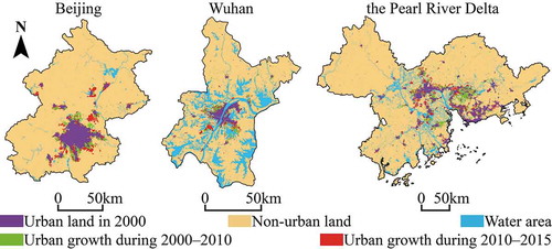
The land-use grid datasets used in this study were provided by the Resource and Environmental Science and Data Center (RESDC) of the Chinese Academy of Sciences (http://www.resdc.cn), and were produced based on Landsat Thematic Mapper (TM) and Enhanced Thematic Mapper Plus (ETM+) remote sensing images. The remote sensing images were first processed through image fusion, geometric correction, image enhancement and mosaicing, and were then classified into six first-class categories and 25 second-class categories through a man-machine interactive visual interpretation technique, with a resolution of 30 m. The six first-class land-use categories were cultivated land, forest land, grassland, water area, construction land (including urban land, rural settlements, and other construction land), and unused land. Among the six first-class categories, the average classification accuracy for the cultivated land and construction land was more than 85%, and the average classification accuracy of the other land-use categories was more than 75%. The specific classification methods for remote sensing data can be found in the studies of Liu et al. (2002), (2010a), (2014a). In this study, the land-use data were reclassified into three categories, i.e. urban land, non-urban land, and water area, with a resolution of 30 m. Figure 1 shows the urban growth of Beijing, Wuhan, and the PRD during 2000–2010 and 2010–2015.

Figure 1. Urban growth for Beijing, Wuhan, and the Pearl River Delta during 2000–2010 and 2010–2015

A series of potential factors influencing urban growth were selected through a literature review (Table 1, Figures S1, S2, and S3). Topographic and environmental factors, proximity factors, socioeconomic factors, and land-use policy and planning have been widely recognized as having significant effects on urban growth (Tan et al. 2014). Topographic and environmental factors, i.e., slope, elevation, the normalized difference vegetation index (NDVI), etc., are usually regarded as the important driving factors that affect urban growth (Müller, Steinmeier, and Küchler 2010; Zhang et al. 2020b). Proximity factors, such as distance to a certain type of land (Wang et al. 2020a), distance to roads (Luo and Wei 2009; Müller, Steinmeier, and Küchler 2010; Poelmans and Van Rompaey 2009), distance to city centers (Vermeiren et al. 2012), and distance to rivers (Luo and Wei 2009), as well as socioeconomic factors, such as the spatial distribution of GDP and population (Wang et al. 2020a), are also crucial driving factors that play a great role in the urbanization process (Tan et al. 2014). For many of the land-use policies and plans in China, such as the eco-environment protection planning, the basic farmland protection regulations, and the “increasing vs. decreasing balance” strategy, they also have a great influence on urban growth. The spatial driving factor data were also provided by the Resource and Environmental Science and Data Center (RESDC) of the Chinese Academy of Sciences (http://www.resdc.cn).

Table 1. Details and generalization of each spatial variable

Datasets	Year	File type	Spatial variables	Meaning of the spatial variables
Urban land	2000	GRID	DIS2UL	Distance to the urban land in 2000
County centers	2010	Shpfile	DIS2CC	Distance to the county centers
National Highways	2010	Shpfile	DIS2NH	Distance to the National highways
Provincial Highways	2010	Shpfile	DIS2PH	Distance to the Provincial Highways
County Highways	2010	Shpfile	DIS2CH	Distance to the County Highways
Super Highways	2010	Shpfile	DIS2SH	Distance to the Super Highways
Railways	2010	Shpfile	DIS2RW	Distance to the Railways
Metros & Light Rails	2010	Shpfile	DIS2MLR	Distance to the Metros & Light Rails
Rivers	–	Shpfile	DIS2RV	Distance to the rivers
NDVI	2010	GRID	NDVI	Distribution of NDVI
GDP	2010	GRID	GDP	Distribution of spatialized GDP
Population	2010	GRID	POP	Distribution of spatialized population
Elevation data	–	GRID	DEM	The elevation of the terrain
Slope data	–	GRID	Slope	The slope of the terrain

Data source: Resource and Environment Science and Data Center (http://www.resdc.cn)

3 Methodology

3.1 Dual-scale neighborhood based on vectorization

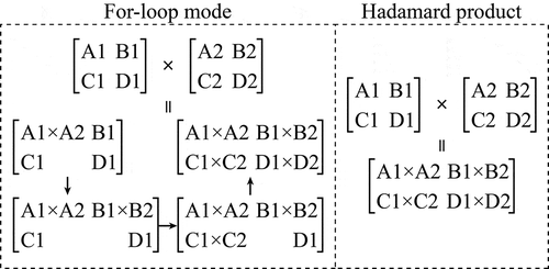
As described previously, the neighborhoods currently used in CA models have a contradiction when characterizing the local interactions. In this paper, a new type of neighborhood is proposed to avoid this contradiction, namely, the DSN, which separates the two functions (peripheral influence receiving and pattern constraining) of the original neighborhood (ORN). The calculation of the DSN effect includes the calculation of the PCN effect, the IRN effect, and their combination, which significantly increases the computation when compared to the calculation of the ORN. Therefore, it is necessary to use vectorization to improve the computational efficiency of the neighborhood calculation. In this study, we adopted a 2-D convolution method to calculate the neighborhood effect, and then used the Hadamard product to couple the effects of the PCN and IRN. These two methods are commonly used in the field of image processing, and can save a lot of computation time (Wu et al. 2011; Xia et al. 2018, 2020b).

The calculation principle of 2-D convolution is shown in Figure 2, where the convolution operations in Location 1 and Location 2 can be computed at the same time by the computer, which greatly improves the computational efficiency. In this study, the CA models were constructed on the MATLAB R2015b platform, and the 2-D convolution process was performed by the conv2(·) function in the function library of MATLAB. The calculation principle for the Hadamard product is shown in Figure 3, where it can be seen that using the Hadamard product method to multiply the two matrices needs only one operation, whereas matrix multiplication in for-loop mode needs four operations, which makes the computation of the Hadamard product method more efficient. The pseudo-code of the algorithm for calculating the effect of the DSN based on vectorization is shown in Algorithm 2, and the serial/scalar algorithm is shown in Algorithm 1.

Table

Algorithm 1. The pseudo-code of the serial scalar algorithm for calculating the effect of DSN

Input dataset;//the matrix of land-use data is input. for i ← 1 to ncols do for j ← 1 to nrows do if cell(i,j) is a cell of target category or Nodata cells then//exclude NoData cells and the existing cells of target category DSN(i,j) ← 0; else for i ← max(1,i-PCNRadius) to min(i+ PCNRadius,ncols) do//PCN columns. for j ← max(1,j-PCNRadius) to min(j+ PCNRadius,nrows) do//PCN rows. Counter1(i,j) ← Counter1(i,j) + 1;//count the cells of target category in the PCN PCN(i,j) ← Counter1(i,j)/PCNNum;//the calculation of PCN effect for i ← max(1,i–IRNRadius) to min(i+ IRNRadius,ncols) do//IRN columns. for j ← max(1,j-IRNRadius) to min(j+ IRNRadius,nrows) do//IRN rows. Counter2(i,j) ← Counter2(i,j) + 1;//count the cells of target category in the IRN IRN(i,j) ← Counter2(i,j)/IRNNum;//the calculation of IRN effect DSN(i,j) ← PCN(i,j)×IRN(i,j);//the combination of PCN and IRN effects Output dataset;//the DSN effect matrix for target land-use category is output.

Table

Algorithm 2. The pseudo-code of the algorithm for calculating the effect of DSN based on vectorization

Input dataset;//the matrix of land-use data is input. dataset(if dataset ≠ target land-use category code) ← 0;//reclassify the dataset with value 0 meaning other land-use categories. dataset(if dataset = target land-use category code) ← 1;//reclassify the dataset with value 1 meaning target land-use category. PCN_kernel ← a PCNsize-by-PCNsize matrix of ones;//create the PCN in the form of kernel matrix. PCN_kernel((PCNsize+1)/2, (PCNsize+1)/2) ← 0;//exclude the influence of the central cell itself. PCNNum ← PCNsize*PCNsize-1;//the number of cells in the PCN. IRN_kernel ← an IRNsize-by-IRNsize matrix of ones;//create the IRN in the form of kernel matrix. IRN_kernel((IRNsize+1)/2, (IRNsize+1)/2) ← 0;//exclude the influence of the central cell itself. IRNNum ← IRNsize*IRNsize-1;//the number of cells in the IRN. PCN ← conv2(dataset, PCN_kernel)/PCNNum;//PCN effect calculation, and conv2(•) means the 2-D convolution process. IRN ← conv2(dataset, IRN_kernel)/IRNNum;//IRN effect calculation, and conv2(•) means the 2-D convolution process. DSN ← PCN.×IRN;//the combination of PCN and IRN effects, and .× means the Hadamard product. Output dataset;//the DSN effect matrix for target land-use category is output.

Figure 2. Schematic diagram of the 2-D convolution process

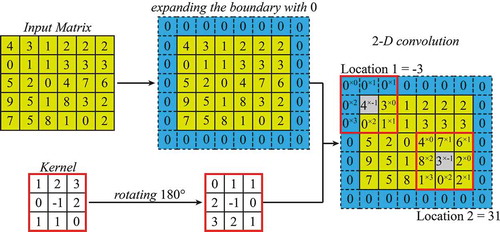
Figure 3. Schematic diagrams of matrix multiplication in for-loop mode and the Hadamard product

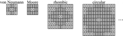
When the 2-D convolution method is applied to the calculation of the neighborhood effect, the input matrix should be a land-use map, with a value of 1 meaning cells of the target land-use category and a value of 0 meaning other cells. The size of the kernel should also be equal to the neighborhood size, and the value of the central cell in the kernel matrix should be 0, in order to exclude the influence of the central cell itself. When the simulated results produced by different neighborhoods need to be compared, the user only needs to change the kernel matrix, so the 2-D convolution method is very suitable for the calculation of neighborhood effects. Figure 4 shows the different neighborhood structures in the form of the kernel matrix. The distribution of positions with a value of 1 represents the range of the neighborhood. Several types of neighborhood can be designed according to this principle, such as the von Neumann neighborhood, the Moore neighborhood, the rhombic neighborhood, and the circular neighborhood. As the Moore neighborhood is the most widely used neighborhood, the ORN, PCN, and IRN in this study were all neighborhoods of Moore type. For the target land-use category m, the neighborhood effects calculated by the ORN and DSN can be represented as:

(1) $\left\{\begin{array}{c}OR{N}_{(u,v),m}=\frac{Count(C_{(u_0,v_0)}=m)}{ORNsize\times ORNsize-1}m=(1,2,3,\dots ,l)\\ DS{N}_{(u,v),m}=\frac{Count(C_{(u_1,v_1)}=m)}{PCNsize\times PCNsize-1}\times \frac{Count(C_{(u_2,v_2)}=m)}{IRNsize\times IRNsize-1}m=(1,2,3,\dots ,l)\end{array}\right.$(1)

Figure 4. The von Neumann neighborhood, Moore neighborhood, rhombic neighborhood, and circular neighborhood in the form of a kernel matrix

where ORN_(u,v),m and DSN_(u,v),m are the neighborhood effects for land-use category m at cell(u,v) calculated by the ORN and DSN, respectively; Count(·) is a counter to calculate the number of cells that belong to land-use category m in the neighborhood; l represents the number of land-use categories; C(u₀,v₀), C(u₁,v₁), and C(u₂,v₂) represent the cell states of the cells in the ORN, PCN, and IRN, respectively; and ORNsize, PCNsize, and IRNsize are the neighborhood sizes of the ORN, PCN, and IRN, respectively.

3.2 DSN-CA model based on the PSO algorithm

CA models can be made up of different components for different purposes, but the transition rule is always the core component (Wang et al. 2013). The transition rules of CA models are constructed by integrating the effects of the land development suitability (LDS), dual-scale neighborhood (DSN), ecological restrictive constraint (ERC) (such as the restrictions of ecological reserves and water areas), and stochastic perturbation (SP) (Wang et al. 2020a). Specifically, the effect of the DSN was coupled with the PCN effect and IRN effect (as described in Equation (1)(1) $\left\{\begin{array}{c}OR{N}_{(u,v),m}=\frac{Count(C_{(u_0,v_0)}=m)}{ORNsize\times ORNsize-1}m=(1,2,3,\dots ,l)\\ DS{N}_{(u,v),m}=\frac{Count(C_{(u_1,v_1)}=m)}{PCNsize\times PCNsize-1}\times \frac{Count(C_{(u_2,v_2)}=m)}{IRNsize\times IRNsize-1}m=(1,2,3,\dots ,l)\end{array}\right.$(1) ) in this study. For the specific descriptions and explanations of the other effects, we refer the reader to White and Engelen (1994), Wu (2002), and Zhang et al. (2020a). The transition rules can be represented as:

(2) $\left\{\begin{array}{c}{P}_{(u,v)}^T=LD{S}_{(u,v)}\times DS{N}_{(u,v)}^T\times ER{C}_{(u,v)}\times S{P}_{(u,v)}^T\\ C_{(u,v)}^{T+1}=\left\{\begin{array}{c}\mathrm{u}\mathrm{r}\mathrm{b}\mathrm{a}\mathrm{n},P_{(u,v)}^T>P_{thred}\\ \mathrm{n}\mathrm{o}\mathrm{n}-\mathrm{u}\mathrm{r}\mathrm{b}\mathrm{a}\mathrm{n},P_{(u,v)}^T\le P_{thred}\end{array}\right.\end{array}\right.$(2)

where $P_{(u,v)}^T$ is the land conversion probability of cell(u,v) at time T; LDS_(u,v) and ERC_(u,v) are the effects of the land development suitability and ecological restrictive constraint at cell(u,v), respectively, which remain constant during the CA iterations; $DS{N}_{(u,v)}^T$and$S{P}_{(u,v)}^T$are the effects of the DSN and SP at cell(u,v) and time T, respectively, which update with the CA iterations; $C_{(u,v)}^{T+1}$is the cell state of cell(u,v) at time T + 1; and P_thred is the probability threshold for the land type conversion. The LDS can be calculated by many methods, such as logistic regression (Wang et al. 2020a), artificial neural networks (Silva et al. 2020), and heuristic optimization algorithms (ZiaeeVafaeyan, Moattar, and Forghani 2018). Based on logistic regression, the LDS can be represented as:

(3) $LDS=\frac{1}{1+exp(-(a+{\sum }_k{b}_k{x}_k))}$(3)

where x_k is the k-th spatial driving factor, b_k is its weight coefficient, and a is a constant. In other words, a and b_k are the parameters of a CA model that define the effects of the spatial driving factors on the land-use change. In this study, near-optimal CA parameters of a and b_k were automatically searched using the PSO algorithm.

The PSO algorithm is a type of evolutionary algorithm which is derived from social behavior simulation. It has a powerful ability to capture the complex processes of urban dynamics, and is commonly used to build the transition rules for CA models (Feng et al. 2011; Liao et al. 2014). The explanation of how we obtained near-optimal CA parameters with the PSO algorithm is as follows. Firstly, assume that there are n particles in a high-dimensional search space R, where the number of dimensions of R is equal to the number of near-optimal CA parameters to be obtained. Each particle in R corresponds to a combination of the target parameters, and can be characterized by a set of attribute values, which are the position of the particle, the velocity of the particle changing its position at the current iteration, and the fitness value defined by the fitness function representing the optimization objective (Kennedy and Eberhart 1995). Therefore, the particle of the PSO algorithm can be represented as:

(4) $X_i\left(po{s_i}_0,po{s_i}_1,\dots ,po{s}_{iD};ve{l_i}_0,ve{l_i}_1,\dots ,ve{l}_{iD};F\left(pos\right)\right),X_i\in R$(4)

where X_i represents the i-th particle (i = 1,2, …, n); D represents the number of dimensions of the search space R; pos = (pos_i0,pos_i1, …, pos_iD) is the position of X_i; vel_i0,vel_i1, …, vel_iD is the velocity of X_i changing its position; and F(pos) is the fitness function whose value guides the optimization process.

At each iteration, there are two kinds of best positions that can be achieved in R. The best position of X_i can be written as BP_iD = (BP_i1, BP_i2, …, BP_iD), and the best position of all X can be written as BP_gD = (BP_g1, BP_g2, …, BP_gD). BP_iD represents the local best fitness value, and BP_gD represents the global best fitness value. Based on the two fitness values, X_i updates its position and velocity as follows (Shi and Eberhart 1998):

(5) $\left\{\begin{array}{c}ve{l}_{iD}(t+1)=w\times ve{l}_{iD}(t)+\text{break}{c}_1\times rand()\times (B{P}_{iD}(t)-po{s}_{iD}(t))+c_2\times rand()\\ \times (B{P}_{gD}(t)-po{s}_{gD}(t))\\ po{s}_{iD}(t+1)=po{s}_{iD}(t)+ve{l}_{iD}(t)\end{array}\right.$(5)

where pos_iD(t), pos_iD(t + 1), vel_iD(t), and vel_iD(t + 1) are the positions and velocities of X_i at time t and t + 1, respectively; w is the inertia coefficient, which represents the effect of vel_iD(t) on vel_iD(t + 1); c₁ and c₂ are constant coefficients adjusting the maximum step lengths of the global and local best particles, respectively; and rand() is a function producing a random number in the range [0, 1]. With the new position and velocity of X_i calculated, the local and global best fitness values at time t + 1 can be defined according to the following (Shi and Eberhart 1998):

(6) $\left\{\begin{array}{c}B{P}_{iD}(t+1)=\left\{\begin{array}{c}po{s}_{iD}(t+1)F(po{s}_{iD}(t+1))\ge F(B{P}_{iD}(t))\\ B{P}_{iD}(t)F(po{s}_{iD}(t+1))<F(B{P}_{iD}(t))\end{array}\right.\\ B{P}_{gD}(t+1)=max(B{P}_{iD}(t+1)),i=1,2,\dots ,n\end{array}\right.$(6)

where BP_iD(t + 1) and BP_gD(t + 1) are the local and global best fitness values at time t + 1, respectively. F(·) is the function calculating the fitness value. In terms of obtaining the near-optimal CA parameters, the fitness function can be constructed as:

(7) $F(b_k)=\sum _j^{ns}{(P_j(b_k)-S_j)}^2$(7)

where ns is the number of samples participating in the PSO algorithm training; b_k is a coefficient vector containing the constant and the weight coefficients of the k spatial driving factors; P_j(b_k) is the LDS calculated in the logistic regression manner (see Equation (3)(3) $LDS=\frac{1}{1+exp(-(a+{\sum }_k{b}_k{x}_k))}$(3) ); S_j is the class label of sample j, with a value of 1 meaning that sample j is a positive sample, i.e., a newly growing cell during the observation, whereas a value of 0 means that sample j is a negative sample, i.e., one of other cells. After using the weight coefficients of the spatial driving factors to encode the particle space, the best configuration of these coefficients can be found in the local and global best positions of the particle space under the guidance of minimizing the fitness function value (Feng et al. 2011; Liao et al. 2014; Rabbani, Aghababaee, and Rajabi 2012).

3.3 Assessment methods

The FoM and LSI were used to evaluate the simulation results with regard to accuracy and landscape, respectively. The FoM indicates the model performance, focusing on the change, and is defined as the ratio of the intersection and union of the actual result and the predicted result (Pontius et al. 2008; Zhang et al. 2020a). The FoM is widely used in the comparison of the actual and simulation results of CA models. The LSI was used to evaluate the shape complexity of the simulated landscape in this study (McGarigal, Cushman, and Ene 2012). It represents the shape deviation between the simulated patch and a square of the same acreage. The calculation of the FoM and LSI can be represented as:

(8) $\left\{\begin{array}{c}FoM=\frac{B}{A+B+C+D}\\ LSI=\frac{0.25\times Edge}{\sqrt{Area}}\end{array}\right.$(8)

where A is the area of error due to observed change predicted as persistence, B is the area of correctness due to observed change predicted as change, C is the area of error due to observed change predicted as change to the wrong category (here C should be set to 0 because this study only considered urban land as the target land-use category, to simulate the process of non-urban cells changing to urban cells), and D is the area of error due to observed persistence predicted as change (He et al. 2018). LSI is the landscape shape index, Edge is the total length of edge of the simulated landscape patches, and Area is the total acreage of the simulated landscape patches.

4 Results

4.1 CA parameter training and model configuration

In this study, the CA models were configured as follows. The land-use data were first reclassified into three categories, i.e. urban, non-urban, and water area, and the urban land was selected as the target land-use category to simulate its change and examine the advantages of the DSN. The cells of the CA models constructed in this study were the grid cells of the raster data, the cell states were their land-use categories (i.e. urban, non-urban, and water area), and the cell space was the geographic space of the study area (i.e. Beijing, Wuhan, and the PRD). The neighborhood was constructed by the ORN or DSN with different sizes. The time change in the CA models was characterized by the iteration and its time step, and the time step of the iteration was set as half a year, i.e., 20 iterations and 10 iterations were conducted for the calibration (2000–2010) and validation (2010–2015), respectively. The water area was used as the ERC in this study, i.e., if a cell was located in a water area, its cell state could not be changed during the simulation process. The SP was introduced into the CA models in the form of the stochastic variable proposed by White and Engelen (1994), and the parameter controlling the intensity of the SP was set to 2.

The urban growth of Beijing, Wuhan, and the PRD during 2000–2010 and 2010–2015 was established by overlaying the land-use maps of the three periods (Figure 1). The urban growth during 2000–2010 was used to calibrate the transition rules of the CA models, and then the obtained transition rules were validated by simulating the urban growth for 2010–2015. The PSO algorithm is a kind of machine learning algorithm, which shows a better classification performance for balanced training samples (He and Garcia 2009), so 5000 positive samples (urban growth cells, class label = 1) and 5000 negative samples (other cells, class label = 0) were selected from the urban dynamics during 2000–2010 using the random sampling method.

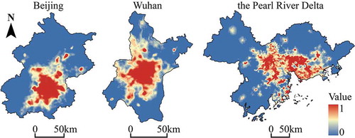
Before PSO algorithm training, the correlations between the spatial variables and urban growth were detected by Spearman’s rank correlation coefficients in SPSS 19.0. The correlations between urban growth and all the selected spatial variables were significant at the 0.01 confidence level (Table S1), indicating that the selection of spatial driving factors was reasonable. The PSO algorithm was run 10 times for each sample set to obtain a result with high reliability. Figure 5 shows the 10 convergence curves of the PSO algorithm training for Beijing, Wuhan, and the PRD, which are relatively stable and yield the best fitness function values at the early and middle states of the optimization process. Figure 6(a) shows the box-plots of the CA parameters obtained from the 10 runs of PSO algorithm training. The variation range of each parameter is small, and there are only a few outliers, indicating that the results of the PSO algorithm training are reliable and the final outcomes are not sensitive to changing weight coefficients. The result with the minimum fitness function value after 1000 generations was used as the final result. Table 2 shows the best trained CA parameters and the corresponding mean squared error (MSE) values of the PSO algorithm training for Beijing, Wuhan, and the PRD. Figure 6(b) shows the receiver operating characteristic (ROC) curves and the area under the curve (AUC) values of the final result. The small MSE together with the large AUC confirms the good performance of the PSO algorithm training. The LDS was calculated according to Equation (3)(3) $LDS=\frac{1}{1+exp(-(a+{\sum }_k{b}_k{x}_k))}$(3) , and is shown in Figure 7 after linear normalization, which can be described as y’ = (y-min(y))/(max(y)-min(y)), where y is the original value and y’ is the normalized value. The spatial variables were also normalized in the same way (see Figures S1, S2, and S3).

Table 2. The best trained CA parameters and the corresponding mean squared error (MSE) values of the PSO algorithm training for Beijing, Wuhan, and the Pearl River Delta

Spatial variables	Beijing	Wuhan	The PRD
Constant	12.624	18.826	8.186
DIS2UL	−14.159	−10.138	−20.240
DIS2CC	2.462	−1.475	−0.476
DIS2NH	4.194	13.090	2.501
DIS2PH	4.682	−11.676	−0.601
DIS2CH	−0.174	−4.936	−9.631
DIS2SH	−8.088	7.918	−5.533
DIS2RW	−9.686	−15.412	−7.427
DIS2MLR	−7.508	−9.174	−1.635
DIS2RV	3.488	0.451	3.033
NDVI	−23.052	−19.981	−12.999
GDP	−0.798	6.460	17.745
POP	20.130	18.649	−14.705
DEM	−1.269	7.341	2.983
Slope	6.570	−17.912	2.176
MSE	0.087	0.118	0.090

Figure 5. The convergence curves of PSO algorithm training for Beijing, Wuhan, and the Pearl River Delta

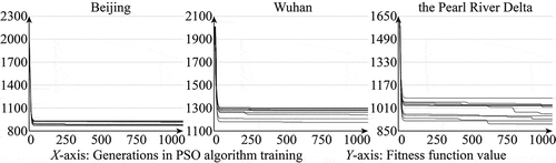
Figure 6. Evaluation of the performance of the PSO training: (a) is the box plot of the CA parameters obtained in the 10 runs of PSO algorithm training; and (b) is the ROC curve of the best result in the 10 runs of PSO algorithm training

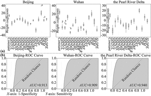
Figure 7. The land development suitability (LDS) of the land cells for Beijing, Wuhan, and the Pearl River Delta

4.2 Dual-scale neighborhood configuration

A series of neighborhood sizes (5, 7, 9, 11, 21, 31 … 201, from 11 to 201 with an increment of 10) were used to simulate the urban growth of Beijing, Wuhan, and the PRD. Each CA model was run 10 times to avoid noise. The FoM and LSI values in Figure 8 are the average values of 10 repetitions. As the neighborhood size changes, the variation of the calibrated FoM and LSI is similar to that of the validated FoM and LSI. With the increase of the neighborhood size, the calibrated and validated FoM values of ORN-CA both first increase and then decrease, while the calibrated and validated LSI values of ORN-CA both keep growing and become far from the values of the actual land-use data. These associated changes of the FoM and LSI with the neighborhood size indicate that increasing the neighborhood size can improve the simulation accuracy, but too large a neighborhood will be counterproductive, which is because a large neighborhood weakens the ability of the CA model to characterize the local interactions and aggravates the shape complexity of the simulated urban landscape. If the modeler desires a high simulation accuracy, they would need to choose a large neighborhood size, but this choice would make the simulation results quite different from the actual urban landscape. Therefore, the DSN is proposed to address this problem, and the DSNsize was recorded by an array [PCNsize, IRNsize] in this study. The primary task of building the DSN is to select a neighborhood size which can produce a simulated urban landscape that is similar to the actual land use (as the PCNsize) through a sensitivity analysis of the neighborhood sizes. As can be seen in Figure 8, the validated urban landscape that is the most similar to the actual one can be obtained with a neighborhood size of 21 for Beijing, a neighborhood size of 5 for Wuhan, and a neighborhood size of 9 for the PRD. Therefore, these values were selected as the PCNsize in DSN-CA for the corresponding study area.

Figure 8. The FoM and LSI values of the simulation results of ORN-CA and DSN-CA with different neighborhood sizes

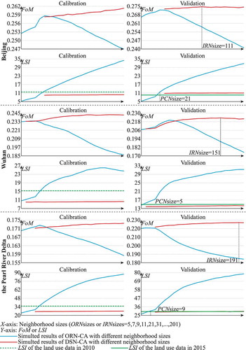
Based on the selected PCNsize values, a series of DSN-CA models with different IRNsize values were constructed to simulate the urban growth of Beijing, Wuhan, and the PRD. With the increase of the IRNsize, the calibrated and validated LSI values for the DSN-CA model remain stable and similar to the actual values, indicating the validity of the pattern constraining function of the DSN. The calibrated and validated FoM values of the DSN-CA model are both larger than those of the ORN-CA model at most neighborhood sizes, and they increase slightly with the IRNsize, which confirms the superiority of the influence receiving function of the DSN. Comparing the calibrated and validated FoM and LSI of the ORN-CA and DSN-CA models, the simulated urban landscape of the DSN-CA model is more similar to the actual urban landscape and the simulation accuracy is higher, which indicates that the contradiction mentioned previously can be addressed by incorporating the DSN into CA models. With the PCNsize determined, the appropriate IRNsize, i.e., the IRNsize with the highest validation accuracy among the tested neighborhood sizes, was chosen by the sensitivity analysis of the IRNsize values. The best DSN for the simulation of the urban growth is the DSN with DSNsize = [21, 111] for Beijing, the DSN with DSNsize = [5, 151] for Wuhan, and the DSN with DSNsize = [5, 151] for the PRD.

4.3 Simulation results and assessment

Three kinds of CA models were constructed to show the advantages of the DSN and the vectorization, namely, the ORN-CA model with the ORNsize equal to the PCNsize, the ORN-CA model with the ORNsize equal to the IRNsize, and the DSN-CA model with the DSNsize equal to [PCNsize, IRNsize]. Comparing the simulation results of the three kinds of CA models for Beijing, Wuhan, and the PRD, the ability of the DSN to capture urban landscapes that are more similar to the actual is apparent, which can be seen in Figure 9 in the zoomed regions of different parts of Beijing, Wuhan, and the PRD.

Figure 9. The simulation results for Beijing, Wuhan, and the Pearl River Delta obtained using the ORN-CA and DSN-CA models

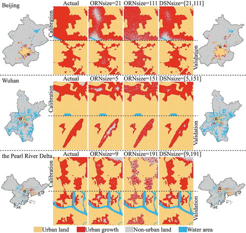
As Liu et al. (2010b), (2014b) described, there are three main types of landscape expansion, namely, infilling, edge-expansion, and outlying. According to this definition, the advantages of the DSN can be considered as its superiority in characterizing the landscape expansion of infilling and edge-expansion, and in avoiding a fragmented landscape. As can be seen in Figure 9, the ORN-CA model with the ORNsize equal to the PCNsize simulates fewer urban growth cells in the regions of infilling and edge-expansion. The ORN-CA model with the ORNsize equal to the IRNsize simulates a larger spatial distribution range for the urban landscape, but its pattern is too fragmented. This comparison indicates that increasing the neighborhood size has the potential to improve the simulation accuracy, but the simultaneously growing shape complexity of the simulated urban landscape seriously reduces the simulation accuracy and the similarity of the landscape to the actual. The simulation results of the DSN-CA model with the DSNsize equal to [PCNsize, IRNsize] simulates more urban growth cells in the regions of infilling and edge-expansion, and produces a more compact urban landscape with more regular edges, which are closer to the actual landscape. These superiorities of the DSN can also be confirmed by comparing the calibrated and validated FoM and LSI values of the DSN-CA models with those of the ORN-CA models (Figure 8 and Table 3), i.e., the FoM values of the simulation results of the DSN-CA models are higher than those of the ORN-CA models, while the LSI values of the DSN-CA model results are approximately equal to those of the ORN-CA models with the ORNsize equal to the PCNsize. Therefore, overall, the simulation performance of the DSN-CA model is better than that of the ORN-CA model, due to the advantages of the DSN in improving the simulation accuracy and ensuring the shape regularity.

Table 3. The calibrated and validated FoM and LSI values of the simulation results of the ORN-CA and DSN-CA models for Beijing, Wuhan, and the Pearl River Delta

Beijing		ORN-CA(ORNsize = 21)	ORN-CA(ORNsize = 111)	DSN-CA(DSNsize = [21,111])
Calibration	FoM	0.258	0.254	0.259
	LSI	10.261	23.542	9.675
Validation	FoM	0.272	0.258	0.275
	LSI	11.744	23.872	10.983
Wuhan		ORN-CA(ORNsize = 5)	ORN-CA(ORNsize = 151)	DSN-CA(DSNsize = [5,151])
Calibration	FoM	0.233	0.196	0.242
	LSI	10.591	26.043	10.158
Validation	FoM	0.207	0.190	0.223
	LSI	14.538	30.227	14.297
The PRD		ORN-CA(ORNsize = 9)	ORN-CA(ORNsize = 191)	DSN-CA(DSNsize = [9,191])
Calibration	FoM	0.171	0.159	0.173
	LSI	23.853	86.090	26.870
Validation	FoM	0.221	0.185	0.227
	LSI	30.704	77.692	30.126

Table 4 shows the time required for the urban growth simulation of Beijing, Wuhan, and the PRD, as conducted by the ORN-CA model and DSN-CA model using the different algorithms (see Section 3.1). The ORN-CA and DSN-CA models were implemented in MATLAB R2015b, on a laptop with an AMD Ryzen 5 4600 H 3.0 GHz CPU, 16 GB memory, and Windows 10. Regardless of the neighborhood size, it takes much less time for the CA models based on the vectorized algorithm to simulate the urban growth of Beijing, Wuhan, and the PRD, compared to the CA models based on the serial/scalar algorithm. Furthermore, the simulation time increases with the neighborhood size, especially when using the serial/scalar algorithm. Although the configuration of the DSN increases the computation and simulation time, the negative impact is almost negligible when using the vectorized algorithm, while the negative impact is significant when using the serial/scalar algorithm. Therefore, the vectorization can greatly improve the simulation efficiency of CA models, and is very suitable for the calculation of the DSN effects in CA models.

Table 4. Time (s) required for the ORN-CA and DSN-CA models to simulate the urban growth of Beijing, Wuhan, and the Pearl River Delta

Beijing	ORN-CA(ORNsize = 21)	ORN-CA(ORNsize = 111)	DSN-CA(DSNsize = [21,111])
Algorithm 1	1337.026	37,060.891	41,103.602
Algorithm 2	35.612	68.598	74.574
Wuhan	ORN-CA(ORNsize = 5)	ORN-CA(ORNsize = 151)	DSN-CA(DSNsize = [5,151])
Algorithm 1	87.584	31,514.460	32,128.646
Algorithm 2	20.476	37.917	39.577
The PRD	ORN-CA(ORNsize = 9)	ORN-CA(ORNsize = 191)	DSN-CA(DSNsize = [9,191])
Algorithm 1	1779.006	296,880.632	320,631.083
Algorithm 2	152.772	392.296	404.487

5 Discussion

Various studies reported that large neighborhood effects existed in the land-use change process, and the simulation accuracy increased with the neighborhood size (Liao et al. 2016; Wu et al. 2012). However, the results of this study showed that too large a neighborhood size is counterproductive. This is because the oversize neighborhood leads the neighborhood effects of the CA model to be more similar to the global effects than the local effects, which weakens the ability of the CA model to characterize the local interactions and increases the shape complexity of the simulated landscape, while reducing the simulation accuracy and the similarity of the simulated landscape to the actual. Comparing the calibrated and validated FoM and LSI values of the simulation results of ORN-CA models at different neighborhood sizes, the contradiction in the selection of neighborhood size has been confirmed, which is that small neighborhoods have the ability to constrain the shape complexity of the simulated landscape, but they cannot sufficiently characterize the effects of the surrounding cells on the central cell, while large neighborhoods do the opposite.

A new type of dual-scale neighborhood (DSN) was proposed to solve the above contradiction under this study. The function of DSN representing the neighborhood effects is divided into two sub-functions, i.e., a pattern constraining function and an influence receiving function, which are implemented by a small neighborhood (PCN) and a large neighborhood (IRN), respectively. When the DSN was used to build CA models, the simulated landscape was more similar to the actual and remained stable, while the simulation accuracy of the DSN-CA model was higher than that of the ORN-CA model. According to the types of landscape expansion classified by Liu et al. (2010b), (2014b), the DSN shows superiority in capturing the landscape expansion of infilling and edge-expansion and in avoiding a fragmented landscape. Furthermore, a vectorized algorithm was adopted to replace the serial/scalar algorithm to calculate the DSN effects, which saves a lot of computation and greatly improves the simulation efficiency of the DSN-CA model.

The proposed DSN based on vectorization was applied to simulate the urban growth of two cities and one urban agglomeration, and the similar results of these study areas showed that the superiority of the proposed approach was spatially transferable and independent of the scale of study areas. It is challenging to determine whether the performance of the approach is still superior when applying it to the simulation involving multiple land-use types. However, the efficiency advantage of the approach can be reasonably inferred to be significant, because the neighborhood effects of CA models involving multiple land-use types are calculated separately according to land-use types, and the neighborhood calculation of each land-use type is the same as that of urban CA models (Lin et al. 2020; Zhang et al. 2019; Liu et al. 2017). There are still several problems to be addressed in future research, for example, it needs further exploration about how the performance of the approach will change while dealing with the simulation over a long span of time. And only the most widely used neighborhood type was considered in this study, namely, the Moore neighborhood. Whether other types of neighborhood such as a von Neumann neighborhood or a circular neighborhood would obtain better effects remains to be studied. Besides, since imposing equal weights on the influences of neighborhood cells on the central cell is imperfect, it is challenging to accurately characterize the influences of peripheral cells, especially for large IRNs.

6 Conclusions

In this paper, we have proposed a new type of dual-scale neighborhood (DSN) based on vectorization to improve the simulation performance and computational efficiency of CA models. The DSN-CA model was successfully applied to simulate the urban growth of Beijing, Wuhan, and the PRD. The datasets used in this research included land-use data of Beijing, Wuhan, and the PRD for 2000, 2010, and 2015, and a series of spatial driving factors. Two CA models, namely, the ORN-CA model (the CA model using the original neighborhood) and the DSN-CA model (the CA model using the DSN), were constructed and compared to show the advantages of the DSN. The two CA models were calibrated by comparing the simulation results for 2010 with the actual data for 2010, and validated by comparing the simulation results for 2015 with the actual data for 2015. Based on the simulation results of the ORN-CA model and DSN-CA model with different neighborhood configurations, the contradiction in the selection of neighborhood size was confirmed, and it was proved that the proposed DSN has the capability to solve this contradiction. We also applied two algorithms, a serial/scalar algorithm and a vectorized algorithm, to calculate the effects of the ORN and DSN, respectively. The simulation times of the two algorithms were also recorded and compared to confirm the efficiency improvement of the vectorization. The results show that incorporating the DSN into a CA model will enable the user to choose the appropriate configuration of neighborhood, so that simulation results can be obtained with a high accuracy, with a landscape that is similar to the actual, improving the simulation performance of the CA model. Furthermore, the time needed for calculating the neighborhood effects increases with the neighborhood size, especially when using the serial/scalar algorithm. The vectorized algorithm can greatly improve the simulation efficiency of the DSN-CA model, which means that integrating vectorization into the DSN configuration is an excellent way to improve the simulation performance and efficiency of CA models.

Data and codes availability statement

The data and codes that support the findings of this study are openly available in [figshare] at [https://doi.org/10.6084/m9.figshare.12987530.v3].

Highlights

A dual-scale neighborhood (DSN) based on vectorization was proposed for CA models.

The contradiction in the selection of neighborhood size can be avoided by using DSN.

Vectorization greatly improves the computational efficiency of neighborhood effects.

The DSN significantly improves simulation performance and efficiency of CA models.

Acknowledgements

This work was supported by the National Natural Science Foundation of China (41571384).

Disclosure statement

No potential conflict of interest was reported by the authors.

Supplementary Material

Supplemental data for this article can be accessed here.

Additional information

Funding

This work was supported by the National Natural Science Foundation of China [41571384].

References

- Abolhasani, S., and M. Taleai. 2020. “Assessing the Effect of Temporal Dynamics on Urban Growth Simulation: Towards an Asynchronous Cellular Automata.” Transactions in GIS 24 (2): 332–354. doi:10.1111/tgis.12601.
- Abouali, M., F. Daneshvar, and A. P. Nejadhashemi. 2016. “MATLAB Hydrological Index Tool (MHIT): A High Performance Library to Calculate 171 Ecologically Relevant Hydrological Indices.” Ecological Informatics 33: 17–23. doi:10.1016/j.ecoinf.2016.03.004.
- Aburas, M. M., Y. M. Ho, M. F. Ramli, and Z. H. Ash’aari. 2016. “The Simulation and Prediction of Spatio-temporal Urban Growth Trends Using Cellular Automata Models: A Review.” International Journal of Applied Earth Observation and Geoinformation 52: 380–389. doi:10.1016/j.jag.2016.07.007.
- Azari, M., A. Tayyebi, M. Helbich, and M. A. Reveshty. 2016. “Integrating Cellular Automata, Artificial Neural Network, and Fuzzy Set Theory to Simulate Threatened Orchards: Application to Maragheh, Iran.” Giscience & Remote Sensing 53 (2): 183–205. doi:10.1080/15481603.2015.1137111.
- Azari, M., and M. A. Reveshty. 2013. “Interference of Human Impacts in Urban Growth Modelling with Transition Rules of Cellular Automata, GIS and Multi-Temporal Satellite Imagery: A Case Study of Maraghe, Iran.” Journal of the Indian Society of Remote Sensing 41 (4): 993–1008. doi:10.1007/s12524-013-0275-2.
- Barredo, J. I., M. Kasanko, N. McCormick, and C. Lavalle. 2003. “Modelling Dynamic Spatial Processes: Simulation of Urban Future Scenarios through Cellular Automata.” Landscape and Urban Planning 64 (3): 145–160. doi:10.1016/S0169-2046(02)00218-9.
- Barreira-Gonzalez, P., M. Gomez-Delgado, and F. Aguilera-Benavente. 2015. “From Raster to Vector Cellular Automata Models: A New Approach to Simulate Urban Growth with the Help of Graph Theory.” Computers Environment and Urban Systems 54: 119–131. doi:10.1016/j.compenvurbsys.2015.07.004.
- Berberoglu, S., A. Akin, and K. C. Clarke. 2016. “Cellular Automata Modeling Approaches to Forecast Urban Growth for Adana, Turkey: A Comparative Approach.” Landscape and Urban Planning 153: 11–27. doi:10.1016/j.landurbplan.2016.04.017.
- Birkbeck, N., J. Levesque, and J. N. Amaral. 2007. A Dimension Abstraction Approach to Vectorization in Matlab. International Symposium on Code Generation and Optimization (CGO'07), San Jose, CA, USA, pp. 115–130. doi:10.1109/CGO.2007.1.
- Cao, M., G. A. Tang, Q. F. Shen, and Y. X. Wang. 2015. “A New Discovery of Transition Rules for Cellular Automata by Using Cuckoo Search Algorithm.” International Journal of Geographical Information Science 29 (5): 806–824. doi:10.1080/13658816.2014.999245.
- Chang, C. Y., and C. C. Ma. 2017. “Increasing the Computational Efficient of Digital Cross Correlation by a Vectorization Method.” Mechanical Systems and Signal Processing 92: 293–314. doi:10.1016/j.ymssp.2017.01.027.
- Chen, J. Z., M. Q. Du, X. J. Qin, and Y. W. Miao. 2018. “An Improved Topology Extraction Approach for Vectorization of Sketchy Line Drawings.” Visual Computer 34 (12): 1633–1644. doi:10.1007/s00371-018-1549-z.
- Dahal, K. R., and T. E. Chow. 2015. “Characterization of Neighborhood Sensitivity of an Irregular Cellular Automata Model of Urban Growth.” International Journal of Geographical Information Science 29 (3): 475–497. doi:10.1080/13658816.2014.987779.
- Ewing, R., G. Tian, and T. Lyons. 2018. “Does Compact Development Increase or Reduce Traffic Congestion?.” CITIES 72 (A): 94–101. doi:10.1016/j.cities.2017.08.010.
- Feng, Y. J., and X. H. Tong. 2018. “Dynamic Land Use Change Simulation Using Cellular Automata with Spatially Nonstationary Transition Rules.” Giscience & Remote Sensing 55 (5): 678–698. doi:10.1080/15481603.2018.1426262.
- Feng, Y. J., and X. H. Tong. 2019. “Incorporation of Spatial Heterogeneity-weighted Neighborhood into Cellular Automata for Dynamic Urban Growth Simulation.” Giscience & Remote Sensing 56 (7): 1024–1045. doi:10.1080/15481603.2019.1603187.
- Feng, Y. J., Y. Liu, and M. Batty. 2016. “Modeling Urban Growth with GIS Based Cellular Automata and Least Squares SVM Rules: A Case Study in Qingpu-Songjiang Area of Shanghai, China.” Stochastic Environmental Research and Risk Assessment 30 (5): 1387–1400. doi:10.1007/s00477-015-1128-z.
- Feng, Y. J., Y. Liu, X. H. Tong, M. L. Liu, and S. S. Deng. 2011. “Modeling Dynamic Urban Growth Using Cellular Automata and Particle Swarm Optimization Rules.” Landscape and Urban Planning 102 (3): 188–196. doi:10.1016/j.landurbplan.2011.04.004.
- Feng, Y. L., and Y. Qi. 2018. “Modeling Patterns of Land Use in Chinese Cities Using an Integrated Cellular Automata Model.” Isprs International Journal of Geo-information 7 (10): 403. doi:10.3390/ijgi7100403.
- He, H. B., and E. A. Garcia. 2009. “Learning from Imbalanced Data.” Ieee Transactions on Knowledge and Data Engineering 21 (9): 1263–1284. doi:10.1109/TKDE.2008.239.
- He, J., X. Li, Y. Yao, Y. Hong, and Z. Jinbao. 2018. “Mining Transition Rules of Cellular Automata for Simulating Urban Expansion by Using the Deep Learning Techniques.” International Journal of Geographical Information Science 32 (10): 2076–2097. doi:10.1080/13658816.2018.1480783.
- Kazemzadeh-Zow, A., S. Z. Shahraki, L. Salvati, and N. N. Samani. 2017. “A Spatial Zoning Approach to Calibrate and Validate Urban Growth Models.” International Journal of Geographical Information Science 31 (4): 763–782. doi:10.1080/13658816.2016.1236927.
- Kennedy, J., and R. Eberhart. 1995. “Particle Swarm Optimization.” Proceedings of ICNN'95 - International Conference on Neural Networks, Perth, WA, Australia, pp. 1942–1948 vol.4, doi:10.1109/ICNN.1995.488968.
- Kocabas, V., and S. Dragicevic. 2006. “Assessing Cellular Automata Model Behaviour Using a Sensitivity Analysis Approach.” Computers Environment and Urban Systems 30 (6): 921–953. doi:10.1016/j.compenvurbsys.2006.01.001.
- Li, X., and A. G. O. Yeh. 2000. “Modelling Sustainable Urban Development by the Integration of Constrained Cellular Automata and GIS.” International Journal of Geographical Information Science 14 (2): 131–152. doi:10.1080/136588100240886.
- Li, X., Y. Chen, X. Liu, X. Xu, and G. Chen. 2017. “Experiences and Issues of Using Cellular Automata for Assisting Urban and Regional Planning in China.” International Journal of Geographical Information Science 31 (8): 1606–1629. doi:10.1080/13658816.2017.1301457.
- Li, X. C., X. P. Liu, and L. Yu. 2014. “A Systematic Sensitivity Analysis of Constrained Cellular Automata Model for Urban Growth Simulation Based on Different Transition Rules.” International Journal of Geographical Information Science 28 (7): 1317–1335. doi:10.1080/13658816.2014.883079.
- Liang, W., and M. Yang. 2019. “Urbanization, Economic Growth and Environmental Pollution: Evidence from China.” Sustainable Computing-informatics & Systems 21: 1–9. doi:10.1016/j.suscom.2018.11.007.
- Liao, J. F., L. N. Tang, G. F. Shao, and X. D. Su. 2014. “A Neighbor Decay Cellular Automata Approach for Simulating Urban Expansion Based on Particle Swarm Intelligence.” International Journal of Geographical Information Science 28 (4): 720–738. doi:10.1080/13658816.2013.869820.
- Liao, J. F., L. N. Tang, G. F. Shao, X. D. Su, D. K. Chen, and T. Xu. 2016. “Incorporation of Extended Neighborhood Mechanisms and Its Impact on Urban Land-use Cellular Automata Simulations.” Environmental Modelling and Software 75 (SI): 163–175. doi:10.1016/j.envsoft.2015.10.014.
- Lin, J. Y., X. Li, S. Y. Li, and Y. Y. Wen. 2020. “What Is the Influence of Landscape Metric Selection on the Calibration of Land-use/cover Simulation Models?.” Environmental Modelling and Software 129: 104719. doi:10.1016/j.envsoft.2020.104719.
- Liu, D. Y., X. Q. Zheng, H. B. Wang, C. X. Zhang, J. Y. Li, and Y. Q. Lv. 2018. “Interoperable Scenario Simulation of Land-use Policy for Beijing-Tianjin-Hebei Region, China.” Land Use Policy 75: 155–165. doi:10.1016/j.landusepol.2018.03.040.
- Liu, J. Y., M. L. Liu, X. Z. Deng, and D. Luo. 2002. “The Land Use and Land Cover Change Database and Its Relative Studies in China.” Journal of Geographical Sciences 12 (3): 275–282. doi:10.1007/BF02837545.
- Liu, J. Y., W. H. Kuang, Z. X. Zhang, and W. F. Chi. 2014a. “Spatiotemporal Characteristics, Patterns, and Causes of Land-use Changes in China since the Late 1980s.” Journal of Geographical Sciences 24 (2): 195–210. doi:10.1007/s11442-014-1082-6.
- Liu, J. Y., Z. X. Zhang, X. L. Xu, and N. Jiang. 2010a. “Spatial Patterns and Driving Forces of Land Use Change in China during the Early 21st Century.” Journal of Geographical Sciences 20 (4): 483–494. doi:10.1007/s11442-010-0483-4.
- Liu, X. P., L. Ma, X. Li, and Z. J. He. 2014b. “Simulating Urban Growth by Integrating Landscape Expansion Index (LEI) and Cellular Automata.” International Journal of Geographical Information Science 28(1):148–163. doi:10.1080/13658816.2013.831097.
- Liu, X. P., X. Li, Y. M. Chen, and B. Ai. 2010b. “A New Landscape Index for Quantifying Urban Expansion Using Multi-temporal Remotely Sensed Data.” Landscape Ecology 25(5):671–682. doi:10.1007/s10980-010-9454-5.
- Liu, X. P., X. Liang, X. Li, and F. S. Pei. 2017. “A Future Land Use Simulation Model (FLUS) for Simulating Multiple Land Use Scenarios by Coupling Human and Natural Effects.” Landscape and Urban Planning 168: 94–116. doi:10.1016/j.landurbplan.2017.09.019.
- Luo, J., and Y. H. D. Wei. 2009. “Modeling Spatial Variations of Urban Growth Patterns in Chinese Cities: The Case of Nanjing.” Landscape and Urban Planning 91 (2): 51–64. doi:10.1016/j.landurbplan.2008.11.010.
- McGarigal, K., S. A. Cushman, and E. Ene. 2012. FRAGSTATS V4: Spatial Pattern Analysis Program for Categorical and Continuous Maps. Amherst: Computer software program produced by the authors at the University of Massachusetts. Available at the following web site: http://www.umass.edu/landeco/research/fragstats/fragstats.html.
- Menard, A., and D. J. Marceau. 2005. “Exploration of Spatial Scale Sensitivity in Geographic Cellular Automata.” Environment and Planning B-planning & Design 32 (5): 693–714. doi:10.1068/b31163.
- Moreno, N., F. Wang, and D. J. Marceau. 2009. “Implementation of a Dynamic Neighborhood in a Land-use Vector-based Cellular Automata.” Computers Environment and Urban Systems 33 (1): 44–54. doi:10.1016/j.compenvurbsys.2008.09.008.
- Müller, K., C. Steinmeier, and M. Küchler. 2010. “Urban Growth along Motorways in Switzerland.” Landscape and Urban Planning 98 (1): 3–12. doi:10.1016/j.landurbplan.2010.07.004.
- Mustafa, A., A. Heppenstall, H. Omrani, I. Saadi, M. Cools, and J. Teller. 2018a. “Modelling Built-up Expansion and Densification with Multinomial Logistic Regression, Cellular Automata and Genetic Algorithm.” Computers Environment and Urban Systems 67: 147–156. doi:10.1016/j.compenvurbsys.2017.09.009.
- Mustafa, A., I. Saadi, M. Cools, and J. Teller. 2018b. “A Time Monte Carlo Method for Addressing Uncertainty in Land-use Change Models.” International Journal of Geographical Information Science 32 (11): 2317–2333. doi:10.1080/13658816.2018.1503275.
- Omrani, H., A. Tayyebi, and B. Pijanowski. 2017. “Integrating the Multi-label Land-use Concept and Cellular Automata with the Artificial Neural Network-based Land Transformation Model: An Integrated ML-CA-LTM Modeling Framework.” Giscience & Remote Sensing 54 (3): 283–304. doi:10.1080/15481603.2016.1265706.
- Poelmans, L., and A. Van Rompaey. 2009. “Detecting and Modelling Spatial Patterns of Urban Sprawl in Highly Fragmented Areas: A Case Study in the Flanders-Brussels Region.” Landscape and Urban Planning 93 (1): 10–19. doi:10.1016/j.landurbplan.2009.05.018.
- Pontius, R. G., and L. C. Schneider. 2001. “Land-cover Change Model Validation by an ROC Method for the Ipswich Watershed, Massachusetts, USA.” Agriculture, Ecosystems & Environment 85 (1–3): 239–248. doi:10.1016/S0167-8809(01)00187-6.
- Pontius, R. G., W. Boersma, J.-C. Castella, and P. H. Verburg. 2008. “Comparing the Input, Output, and Validation Maps for Several Models of Land Change.” Annals of Regional Science 42 (1): 11–37. doi:10.1007/s00168-007-0138-2.
- Rabbani, A., H. Aghababaee, and M. A. Rajabi. 2012. “Modeling Dynamic Urban Growth Using Hybrid Cellular Automata and Particle Swarm Optimization.” Journal of Applied Remote Sensing 6 (1): 063582. doi:10.1117/1.JRS.6.063582.
- Salap-Ayca, S., P. Jankowski, K. C. Clarke, P. C. Kyriakidis, and A. Nara. 2018. “A Meta-modeling Approach for Spatio-temporal Uncertainty and Sensitivity Analysis: An Application for A Cellular Automata-based Urban Growth and Land-use Change Model.” International Journal of Geographical Information Science 32 (4): 637–662. doi:10.1080/13658816.2017.1406944.
- Sante, I., A. M. Garcia, D. Miranda, and R. Crecente. 2010. “Cellular Automata Models for the Simulation of Real-world Urban Processes: A Review and Analysis.” Landscape and Urban Planning 96 (2): 108–122. doi:10.1016/j.landurbplan.2010.03.001.
- Shabanov, B. M., A. A. Rybakov, and S. S. Shumilin. 2019. “Vectorization of High-performance Scientific Calculations Using AVX-512 Intruction Set.” Lobachevskii Journal of Mathematics 40 (5): 580–598. doi:10.1134/S1995080219050196.
- Shafizadeh-Moghadam, H., A. Asghari, M. Taleai, M. Helbich, and A. Tayyebi. 2017. “Sensitivity Analysis and Accuracy Assessment of the Land Transformation Model Using Cellular Automata.” Giscience & Remote Sensing 54 (5): 639–656. doi:10.1080/15481603.2017.1309125.
- Shi, Y. H., and R. Eberhart. 1998. A Modified Particle Swarm Optimizer. 1998 IEEE international conference on evolutionary computation proceedings, IEEE World Congress on Computational Intelligence (Cat. No.98TH8360), Anchorage, AK, USA, pp. 69–73. doi:10.1109/ICEC.1998.699146
- Silva, L. P. E., A. P. C. Xavier, R. M. da Silva, and C. A. G. Santos. 2020. “Modeling Land Cover Change Based on an Artificial Neural Network for a Semiarid River Basin in Northeastern Brazil.” Global Ecology and Conservation 21: e00811. doi:10.1016/j.gecco.2019.e00811.
- Skog, K. L., and M. Steinnes. 2016. “How Do Centrality, Population Growth and Urban Sprawl Impact Farmland Conversion in Norway?.” Land Use Policy 59: 185–196. doi:10.1016/j.landusepol.2016.08.035.
- Stock, K., L. N. Pouchet, and P. Sadayappan. 2012. “Using Machine Learning to Improve Automatic Vectorization.” Acm Transactions on Architecture and Code Optimization 8 (4): 50. doi:10.1145/2086696.2086729.
- Tan, R. H., Y. L. Liu, Y. F. Liu, Q. S. He, L. C. Ming, and S. H. Tang. 2014. “Urban Growth and Its Determinants across the Wuhan Urban Agglomeration, Central China.” Habitat International 44: 268–281. doi:10.1016/j.habitatint.2014.07.005.
- Tayyebi, A., P. C. Perry, and A. H. Tayyebi. 2014. “Predicting the Expansion of an Urban Boundary Using Spatial Logistic Regression and Hybrid Raster-vector Routines with Remote Sensing and GIS.” International Journal of Geographical Information Science 28 (4): 639–659. doi:10.1080/13658816.2013.845892.
- Tobler, W. R. 1970. “A Computer Movie Simulating Urban Growth in the Detroit Region.” Economic Geography 46 (2): 234–240. doi:10.2307/143141.
- Tong, X. H., and Y. J. Feng. 2019. “How Current and Future Urban Patterns Respond to Urban Planning? an Integrated Cellular Automata Modeling Approach.” CITIES 92: 247–260. doi:10.1016/j.cities.2019.04.004.
- Trouve, A., A. J. Cruz, K. J. Murakami, M. Arai, T. Nakahira, and E. Yamanaka. 2016. “Guide Automatic Vectorization by Means of Machine Learning: A Case Study of Tensor Contraction Kernels.” Ieice Transactions on Information and Systems, E 99D (6): 1585–1594. doi:10.1587/transinf.2015EDP7440.
- van Vliet, J., A. K. Bregt, D. G. Brown, and P. H. Verburg. 2016. “A Review of Current Calibration and Validation Practices in Land-change Modeling.” Environmental Modelling and Software 82: 174–182. doi:10.1016/j.envsoft.2016.04.017.
- Vermeiren, K., A. Van Rompaey, M. Loopmans, E. Serwajja, and P. Mukwaya. 2012. “Urban Growth of Kampala, Uganda: Pattern Analysis and Scenario Development.” Landscape and Urban Planning 106 (2): 199–206. doi:10.1016/j.landurbplan.2012.03.006.
- Wahyudi, A., and Y. Liu. 2016. “Cellular Automata for Urban Growth Modelling: A Review on Factors Defining Transition Rules.” International Review for Spatial Planning and Sustainable Development 4 (2): 60–75. doi:10.14246/irspsd.4.2_60.
- Wang, H. J., B. Zhang, C. Xia, S. W. He, and W. T. Zhang. 2020a. “Using a Maximum Entropy Model to Optimize the Stochastic Component of Urban Cellular Automata Models.” International Journal of Geographical Information Science 34 (5): 924–946. doi:10.1080/13658816.2019.1687898.
- Wang, H. J., S. W. He, X. J. Liu, L. Dai, P. Pan, S. Hong, and W. T. Zhang. 2013. “Simulating Urban Expansion Using A Cloud-based Cellular Automata Model: A Case Study of Jiangxia, Wuhan, China.” Landscape and Urban Planning 110: 99–112. doi:10.1016/j.landurbplan.2012.10.016.
- Wang, Y. W., Z. Y. Sha, X. C. Tan, H. Lan, X. F. Liu, and J. Rao. 2020b. “Modeling Urban Growth by Coupling Localized Spatio-temporal Association Analysis and Binary Logistic Regression.” Computers Environment and Urban Systems 81: 101482. doi:10.1016/j.compenvurbsys.2020.101482.
- White, R., and G. Engelen. 1994. “Urban Systems Dynamics and Cellular Automata: Fractal Structures between Order and Chaos.” CHAOS SOLITONS & FRACTALS 4 (4): 563–583. doi:10.1016/0960-0779(94)90066-3.
- White, R., and G. Engelen. 2000. “High-resolution Integrated Modelling of the Spatial Dynamics of Urban and Regional Systems.” Computers Environment and Urban Systems 24 (5): 383–400. doi:10.1016/S0198-9715(00)00012-0.
- Wu, F. L. 2002. “Calibration of Stochastic Cellular Automata: The Application to Rural-urban Land Conversions.” International Journal of Geographical Information Science 16 (8): 795–818. doi:10.1080/13658810210157769.
- Wu, H., L. Zhou, X. Chi, Y. Li, and Y. R. Sun. 2012. “Quantifying and Analyzing Neighborhood Configuration Characteristics to Cellular Automata for Land Use Simulation considering Data Source Error.” Earth Science Informatics 5 (2): 77–86. doi:10.1007/s12145-012-0097-8.
- Wu, H., Z. Li, K. C. Clarke, W. Z. Shi, L. C. Fang, A. Q. Lin, and J. Zhou. 2019. “Examining the Sensitivity of Spatial Scale in Cellular Automata Markov Chain Simulation of Land Use Change.” International Journal of Geographical Information Science 33 (5): 1040–1061. doi:10.1080/13658816.2019.1568441.
- Wu, J., M. F. Lu, Y. C. Dong, M. Zheng, M. Huang, and Y. N. Wu. 2011. “Zero-order Noise Suppression with Various Space-shifting Manipulations of Reconstructed Images in Digital Holography.” Applied Optics 50 (34): H56–H61. doi:10.1364/AO.50.000H56.
- Xia, C., A. Q. Zhang, H. J. Wang, and J. F. Liu. 2020a. “Delineating Early Warning Zones in Rapidly Growing Metropolitan Areas by Integrating a Multiscale Urban Growth Model with Biogeography-based Optimization.” Land Use Policy 90: 104332. doi:10.1016/j.landusepol.2019.104332.
- Xia, C., B. Zhang, H. J. Wang, S. Qiao, and A. Q. Zhang. 2020b. “A Minimum-volume Oriented Bounding Box Strategy for Improving the Performance of Urban Cellular Automata Based on Vectorization and Parallel Computing Technology.” Giscience & Remote Sensing 57 (1): 91–106. doi:10.1080/15481603.2019.1670974.
- Xia, C., H. J. Wang, A. Q. Zhang, and W. T. Zhang. 2018. “A High-performance Cellular Automata Model for Urban Simulation Based on Vectorization and Parallel Computing Technology.” International Journal of Geographical Information Science 32 (2): 399–424. doi:10.1080/13658816.2017.1390118.
- Xu, B., J. P. Chen, and P. P. Yu. 2017. “Vectorization of Classified Remote Sensing Raster Data to Establish Topological Relations among Polygons.” Earth Science Informatics 10 (1): 99–113. doi:10.1007/s12145-016-0273-3.
- Yao, F. M., C. Hao, and J. H. Zhang. 2016. “Simulating Urban Growth Processes by Integrating Cellular Automata Model and Artificial Optimization in Binhai New Area of Tianjin, China.” Geocarto International 31 (6): 612–627. doi:10.1080/10106049.2015.1073365.
- Yeh, A. G. O., and X. Li. 2001. “A Constrained CA Model for the Simulation and Planning of Sustainable Urban Forms by Using GIS.” Environment and Planning B-planning & Design 28 (5): 733–753. doi:10.1068/b2740.
- Yeh, A. G. O., and X. Li. 2002. “A Cellular Automata Model to Simulate Development Density for Urban Planning.” Environment and Planning B-planning & Design 29 (3). doi:10.1068/b1288.
- Yeh, A. G. O., and X. Li. 2006. “Errors and Uncertainties in Urban Cellular Automata.” Computers Environment and Urban Systems 30 (1): 10–28. doi:10.1016/j.compenvurbsys.2004.05.007.
- Zhang, B., H. J. Wang, S. W. He, and C. Xia. 2020a. “Analyzing the Effects of Stochastic Perturbation and Fuzzy Distance Transformation on Wuhan Urban Growth Simulation.” Transactions in GIS 12683. doi:10.1111/tgis.12683.
- Zhang, D. C., X. P. Liu, X. Y. Wu, and Y. M. Chen. 2019. “Multiple Intra-urban Land Use Simulations and Driving Factors Analysis: A Case Study in Huicheng, China.” Giscience & Remote Sensing 56 (2): 282–308. doi:10.1080/15481603.2018.1507074.
- Zhang, Y. H., X. P. Liu, G. L. Chen, and G. H. Hu. 2020b. “Simulation of Urban Expansion Based on Cellular Automata and Maximum Entropy Model.” Science China-earth Sciences 63 (5): 701–712. doi:10.1007/s11430-019-9530-8.
- Zhong, T., Y. Chen, and X. Huang. 2016. “Impact of Land Revenue on the Urban Land Growth toward Decreasing Population Density in Jiangsu Province, China.” Habitat International 58: 34–41. doi:10.1016/j.habitatint.2016.09.005.
- ZiaeeVafaeyan, H., M. H. Moattar, and Y. Forghani. 2018. “Land Use Change Model Based on Bee Colony Optimization, Markov Chain and a Neighborhood Decay Cellular Automata.” Natural Resource Modeling 31 (2): e12151. doi:10.1111/nrm.12151.