Is the protected area coverage still relevant in protecting the Southern Ground-hornbill (Bucorvus leadbeateri) biological niche in Zimbabwe? Perspectives from ecological predictions

ABSTRACT

Examining the suitability of landscape patches for endangered species enhances critical insights and indicators into the processes of population structure, community dynamics, and functioning in ecosystems particularly in protected areas (PAs). While PAs are the cornerstone in biodiversity conservation, there is debate on their efficacy to retain their conservation superiority over unprotected areas under climate change. In the present study, we examined the spatial and temporal effectiveness of PAs at maintaining suitable habitat for the “vulnerable” Southern Ground-hornbill (SGH), Bucorvus leadbeateri compared with the unprotected areas in Zimbabwe. We used a landscape-scale analysis of 182 PAs, their surrounding buffer zones, and unprotected areas coupled with three machine learning models (maximum entropy: MaxEnt, random forest, and support vector machines) to simulate SGH habitat suitability. Bioclimatic, vegetation seasonality and terrain variables were used as predictors against SGH “presence-only” observations and the models were projected for 2050 as future climatic scenarios (i.e. representative concentration pathways: RCP2.6 and RCP8.5). The true skill statistic (TSS) and area under the curve (AUC) were used to evaluate the performance of the modeling framework. Our results show that the PAs network in Zimbabwe is extremely relevant for the conservation of SGH, with 8% of the suitable habitat within PAs projected to become unsuitable by 2050. Higher levels of protection status resulted in higher levels of suitable habitat for the SGH while the suitability of eastern-based PAs showed a decrease and the western-based PAs will potentially increase in suitability. Thus, conservation strategies should take the eastern PAs range contraction and associated westward shift into account. The established potential increase in suitability outside the PAs network (23%–31%) might increase conflicts between agriculture and conservation. We, therefore, suggest an expanded cross-boundary institutional alliance and policy development with all stakeholders to implement a holistic conservation plan. Our work demonstrates the importance of combining multi-source remotely sensed data in predicting habitat suitability for endangered species such as the SGH as key indicators of biological conservation and PAs’ effectiveness.

KEYWORDS:

• Biogeography
• climate change
• ecological niche
• landscape conservation
• machine learning
• protection status
• protected area

1. Introduction

Understanding the drivers of habitat use and the suitability of landscape patches to bird species is crucial in conservation biology as it offers critical perceptions of the processes influencing population dynamics, community structure, and functioning in ecosystems (Muposhi et al. 2016). Landscape use by most avian species is assumed to be adaptive, with an inclination toward areas with conducive vegetation cover, microclimates, and abundant dietary requirements (Moreno et al. 2011). Spatial and temporal habitat suitability and preferential use may further be inclined to physical ecosystem modifications or climate variability (Mudereri et al. 2020a). Similarly, earlier studies show that habitat selection is also determined by environmental quality, competition, predation, water availability, and anthropogenic disturbances (McCarthy, Dwyer, and Mokany 2020; Muposhi et al. 2016). These spatial and temporal dynamics promote heterogeneity in ecosystems that ultimately make them suitable for most bird species in space and time (Muposhi et al. 2016).

Additionally, global climate and land-use changes are likely to trigger numerous species shifts into or outside the “safe hubs” of the boundaries of protected areas (PAs), leading to large species composition turnovers (McCune, Van Natto, and MacDougall 2017; Zhang et al. 2019). PAs are used all over the world as locations that receive legal conservation and protection because of their recognized natural, ecological or cultural values that are critical for in-situ biodiversity conservation, and habitat protection (Manish and Pandit 2019). As of 2016, a total of 202 467 terrestrial PAs were recognized globally, covering approximately 14.8% of the earth’s geographic area (UNEP-WCMC and IUCN 2016). While PAs are used as an important tool in biodiversity conservation, there is an ongoing debate on whether they will retain their ability to conserve biodiversity effectively and efficiently under climate change, as species ranges shift (Eklund et al. 2016; Poor et al. 2019; Lecina-Diaz et al. 2019; Guerra, Rosa, and Pereira 2019). Multiple studies indicate some positive effects of PAs on both terrestrial and marine species under different climate scenarios (Gong et al. 2017; Zomer et al. 2015). However, these case studies do not represent most PAs, particularly those in Africa where climate change impacts are likely to be severe (McCarthy, Dwyer, and Mokany 2020; Mudereri et al. 2020b). Also, African nations tend to have limited budgetary resources and research available to comprehensively protect all the species, particularly avian species which exhibit high sensitivity to environmental change (Lecina-Diaz et al. 2019; Wakelin et al. 2018).

Birds are diverse in taxa within the animal kingdom. However, they are easily driven to extinction by small anthropogenic or natural changes in the environment (Wakelin et al. 2018). Therefore, they can be used as key indicators of small environmental changes, and thus can act as early warning mechanisms for environmental degradation (Kylin, Bouwman, and Evans 2011). Due to the sensitivity of the avian taxa to natural and anthropogenic changes, a large proportion of bird species are in danger of extinction (Araujo et al. 2005). African bird species have already shown massive changes in their distributions in recent decades, often enlarging or contracting their ranges over several hundred kilometers (Walther and van Niekerk 2015). Thus, climate change has greatly influenced the distribution of various bird species, and future climate change will alter the landscapes that will result in the change of habitat, range, distribution, and migration patterns of many bird species (Araujo et al. 2005; Mudereri et al. 2020a). These unprecedented shifts continuously challenge and question the effectiveness of current conservation efforts through PAs (Lecina-Diaz et al. 2019; Guerra, Rosa, and Pereira 2019; McCune, Van Natto, and MacDougall 2017).

In this study, we evaluate and match the current protected area regime and its spatial coverage to the ecological niche of the Southern Ground-hornbill (SGH) Bucorvus leadbeateri, a threatened bird species, using Zimbabwe as a case study. Modeling the distribution and population of species has proved to be a valuable approach in efforts to conserve birds and other animals (Nyakarahuka et al. 2017; Zhang et al. 2019; Feng, Liu, and Tong 2018; Qi, Zhao, and Feng 2010). Niche modeling assumes that the niche of the species is constant over space and time and uses the “presence” or “absence” data with the corresponding bioclimatic and environmental variables and mathematical algorithms to determine potential habitat suitability for a species (Wang et al. 2018). Herein, we use three machine learning techniques for ecological niche modeling namely maximum entropy (Phillips, Anderson, and Schapire 2006), random forest (RF: Breiman 2001), and support vector machines (SVM: Vapnik 1979) to predict and project the niche of the SGH to a new environment i.e. under climate change.

SGH has been reported by other studies as very reliant on protected areas for their reproduction and survival (Broms et al. 2014; Combrink et al. 2017). Hence, the modeling product is matched with the current spatial extent of the designated PAs to create an empirical perspective of the effectiveness of the PAs to safeguard the habitat and niche of the SGH in Zimbabwe. These selected algorithms were used in this study because they have been widely used in conducting complex output predictions and provide relatively high modeling accuracies compared to other machine learning techniques (Abdel-Rahman, Ahmed, and Ismail 2013; Mosomtai et al. 2016; Sarvia, De Petris, and Borgogno-Mondino 2020).

The SGH inhabits savannas mostly in Africa and is presently listed as “vulnerable” under the IUCN red list because of fragmented habitats, degraded landscapes, and persecution (BirdLife International 2020). In South Africa, where most studies on the species have been carried out, it is listed as endangered, similar to the status in Lesotho, Namibia, and Eswatini. The status of the SGH in Kenya, Tanzania, Malawi, Zambia, Zimbabwe, and Mozambique, requires conservation interventions to help increase their numbers. The severe fragmentation of landscapes in and around their preferred forage of open woodlands, savannah grasslands, and woodlands increases the chances of failure in nesting and breeding (Trail 2007; Witteveen et al. 2013). The SGH is a terrestrial, carnivorous, and cooperative breeder generally occurring in groups of between 2 and 11 birds, whose sexual maturity and breeding age takes very long to attain i.e. between 4–10 years (Combrink et al. 2017). Thus, the population decrease is made worse by this slow reproduction of the bird as they reproduce in breeding groups and produce one chick in two to three years (Kemp and Begg 1996).

In Zimbabwe, the fast-rising human population, frequent droughts, and conflicting policies are degrading or modifying previously pristine habitats leading to the destruction of large trees necessary for the reproduction of the SGH (Chiweshe 2007; Witteveen et al. 2013). Further, human and bird conflicts occurring inside and outside of PAs are also a major threat to the SGH within buffer zones of protected areas and beyond. These conflicts include deforestation and agricultural expansion which lead to losses in nesting sites, and unsustainable harvesting of the SGH for traditional medicine (Chiweshe 2007). Also, due to an increase in the elephant population in PAs, the elephants have been reported to be causing significant structural changes of vegetation, with downstream impacts on bird species reliant on some of these tree species (Gandiwa et al. 2011; Valeix et al. 2011). Lately, severe droughts that have frequented southern Africa in the last decade have also caused a significant loss in the population of SGH in Zimbabwe (Witteveen et al. 2013).

In this study, we hypothesized that PAs would effectively represent and hence maintain a suitable habitat for SGH than unprotected areas under a changing climate. Through quantifying the change in modeled habitat suitability instead of the changes in abundance, we examined whether the habitat remained more suitable within PAs (with varying degrees of protection) than surrounding areas under the projected climate changes. We assumed that the structure and systems determining the effectiveness of the PAs is the degree of shield they provide to the suitable habitat. This study is relevant and timely as most studies on the SGH have been conducted in South Africa while very few studies and surveys have been conducted in Zimbabwe. There is therefore a great need for more recent work and consideration to this vulnerable species to bring to the attention of decision-makers and conservationists the need to conserve the remaining suitable habitat.

2.Methodology

2.1. Study area

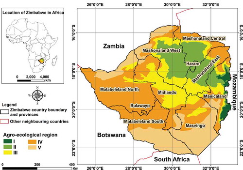
The effectiveness of the protected area approach to conserving SGH suitable habitat was examined in Zimbabwe, a southern African country encompassing ~ 390 753 km² land area. The country occurs within latitudes 15.6^° and 22.4^° S and longitude 25.2^° and 33.1^° E (Mudereri et al. 2020b). The country has five agro-ecological regions (Figure 1) classified based on mean annual rainfall, length of the agricultural growing season, and soil type (Mugandani et al. 2012). Agroecological region “V” receives the lowest mean annual rainfall (400 mm) while agroecological region “I” located on the eastern border with Mozambique receives the highest mean annual rainfall (1 200 mm). Generally, the climatic conditions of the country are subtropical, determined by latitude differences, which distinguishes the wide-ranging rainfall and temperature patterns. The mean annual temperature ranges from 16° C in regions “I” and “II” to ~ 26–35° C in the southern Lowveld. Zimbabwe experiences a short cold, dry season between May and September, while the period November to April is marked by heavy rainfall.

Figure 1. Location of Zimbabwe in Africa and the relative location and boundaries of the five agro-ecological regions of the country which characterize the study area. The map was developed using QGIS software (https://www.qgis.org/en/site/). Adapted from (Mudereri et al. 2020b)

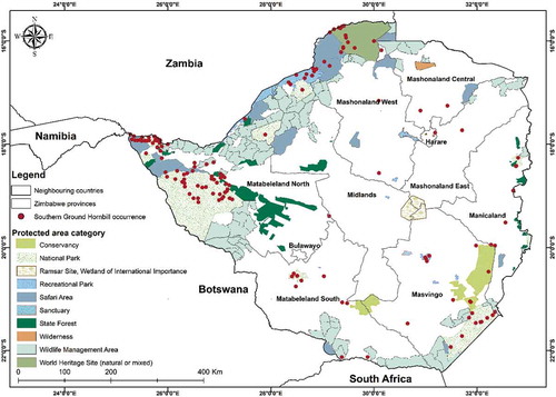
Approximately 182 pieces of land of varying size and protection status covering ~13% of this total land area in Zimbabwe, are designated as PAs (Figure 2). These areas predominantly exist in agroecological region “V” where conventional crop agriculture is limited due to unsuitable climatic conditions. The exact estimated population of the SGH is relatively unknown but is registered as decreasing across its entire African range (BirdLife International 2020)

Figure 2. Location of protected areas in Zimbabwe. The red dots show the distribution of the SGH collated over many years through the global biodiversity information facility (GBIF). The map was developed using QGIS software (https://www.qgis.org/en/site/)

2.2. SGH occurrence data collection

The baseline SGH distribution data in Zimbabwe (n = 380) were collected from the Global Biodiversity Information Facility (GBIF: GBIF 2019). The GBIF (https://www.gbif.org) is one of the major online access point databases providing species occurrence data from billions of biological specimen records obtained through field observations by institutions across the world (Zhang et al. 2019). The data were filtered to eliminate duplicate samples, samples without detailed location information, and those that were too old (year < 1990). Further, to reduce sampling bias, only one sample was kept for each 1 km x 1 km grid to match the resolution of the environmental variables as suggested by Phillips et al. (2009). The latitude and longitude of the retained samples (n = 125) with detailed location information were verified on the Google Earth platform (https://www.google.com/earth/). The retained independent occurrences of SGH were saved in the shapefile (.shp) format and used in the modeling.

2.3. Predictor variables

Predictor variables (n = 35) were grouped into two main categories, i.e. remotely sensed variables (n = 16) and bioclimatic (n = 19), (Tables S1 and S2).

2.4. Bioclimatic variables

Bioclimatic variables are a set of standardized datasets derived from precipitation and temperature values into ecologically useful variables for primary production-based species modeling. These variables, therefore, represent annual tendencies such as average annual temperature and precipitation values and their variations, seasonal characteristics such as temperature and precipitation ranges in the wettest, driest, hottest, and coldest quarters and extremes (O’Donnell and Ignizio 2012). Bioclimatic conditions particularly temperature and precipitation influence the availability of feed, nesting success, thermoregulation, foraging behavior, and reproduction regimes in many bird species including the SGH. This results in the choice or preference of suitable habitats by the SGH. However, these areas with the suitable conditions preferred by the SGH are likely to change soon because of climate change. Hence, the new climatic conditions induced by climate change will ultimately determine the potential shift in habitat for this species. The 19 bioclimatic variables (Table 1 and S1) used in this study were downloaded from the WorldClim platform (www.worldclim.org) at ~1 km x 1 km spatial resolution (Booth 2018; Fick and Hijmans 2017). Two of the four representative concentration pathways (RCPs) set by the intergovernmental panel on climate change (IPCC) using the total radioactive forcing of values 2.6, 4.5, 6, and 8.5 watt/m² (IPCC 2014) were used as future climatic scenarios. Specifically, the current bioclimatic data (1950–2000) and a fourth version of the community climate system model (CCSM4) derived from a one-time step i.e. 2050 (average of predictions for 2041–2060) of the future climate data on the minimum (based on the Paris Agreement targets) and maximum (worst case) emission i.e. RCP2.6 and RCP8.5 were used to capture the whole range of future climate possibilities. The data were clipped to the Zimbabwean country boundary while the pixel size (250 m x 250 m) was matched to the remotely sensed variables pixel size and extents.

Table 1. Bioclimatic and remotely sensed variables used in the final habitat suitability models for the SGH and their (variance inflation factor) VIF values

Variable name	Variable description	Unit	VIF value
	Bioclimatic variables
Bio3	Iso-thermality (Bio2/Bio7) (×100)		2.32
Bio4	Temperature seasonality (standard deviation ×100)		2.33
Bio5	Maximum temperature of the warmest month	^0C	7.67
Bio15	Precipitation seasonality (coefficient of variation)		8.41
Bio18	Precipitation of warmest quarter	mm	5.62
	Land surface temperature
LST	Land surface temperature	K	1.17
	Seasonality variables
Base value	Average minimum enhanced vegetation index (EVI) value	EVI value	5.20
End of season	Time at the end of season	EVI value	2.95
Length of season	Time-lapse from start to end of season	Days	5.30
Start of season	Time of season start	EVI value	2.96
	Topography variables
Aspect	Slope direction	Degrees	1.14
Elevation	Ground height above sea level	m	5.21
Hill shade	Shading the sun effect		1.15
Slope	Ground steepness	%	1.64

2.5. Remotely sensed variables

Three categories of the remotely sensed variables were used in this analysis namely: land surface temperature (LST), topography, and vegetation phenological (vegetation seasonality) variables (Table 1). These variables were selected to test the influence of various environmental determinants on the distribution of SGH. All the remotely sensed variables were standardized to the 250 m x 250 m pixel size using the nearest neighbor method. The nearest neighbor approach assigns a value to each “corrected” pixel from the nearest “uncorrected” pixel. The advantages of nearest neighbor include simplicity and the ability to preserve original values in the unaltered scene.

The “daytime” Land Surface Temperature Climate Modeling Grid (LST_Day_CMG) available from https://lpdaac.usgs.gov/products/mod11c2v006/ was used to represent the LST (Wan, Hook, and Hulley 2015). The “multi-day” MOD11C2 LST product of 5.6 km x 5.6 km spatial resolution available from the year 2000 to the present was used. It was hypothesized that the surface fluxes represented by the LST would influence the general foraging, availability of feed, reproduction, and thus, occurrence and habitat suitability of the SGH. The topography variables were generated from the Shuttle Radar Topographic Mission (SRTM) data which are available at ~ 90 m pixel size digital elevation model (DEM) with a vertical error of less than 16 m (CGIAR-CSI 2019). Aspect, hill-shade, and slope were then derived from the DEM using the “terrain analysis” plugin in QGIS (QGIS Development Team 2019). Elevation, slope, hill-shade, and aspect were expected to influence the occurrence and propagation of SGH by affecting the vegetation and the angle, direction, and intensity of the sun on the earth’s surface.

Vegetation type determines the availability of trees for nesting and foraging sites for the SGH (Kemp and Begg 1996). The specific tree species information was not available, hence the vegetation phenology was used as a proxy for the availability of trees for nesting. The TIMESAT software (Eklundh and Jönsson 2017) was used to derive the seasonal vegetation dynamics. The 250-m MODIS 16-day enhanced vegetation index (EVI) time-series composites obtained between the years 2012 and 2018 were used as inputs into the TIMESAT model. This period coincided with most “presence” points obtained from GBIF. The selection of EVI over the commonly used normalized vegetation index (NDVI) was based on the ability of EVI to enhance vegetation spectral signal and improve spectral sensitivity to high biomass, which is the major weakness of NDVI that tends to saturate in high biomass regions (Zoungrana et al. 2015). In addition, EVI reduces background and atmospheric noises and is more responsive to leaf area index, canopy type, canopy architecture, and plant physiognomy. TIMESAT computes the time-series and performs curve smoothing functions to extract the seasonality parameters from the multi-temporal data using established equations (Eklundh and Per 2017). This sequentially decreases the effects of residual signal noise that exists within the raw EVI time-series data (Hentze, Thonfeld, and Menz 2016). In this study, the Savitzky-Golay filtering equation (Eklundh and Per 2017) was used for fitting, smoothening curves and to remove outliers using a 3- and 5-point window over 2 fitting steps, 3.0 adaptation strength without a spike or amplitude cutoff, a 0.0 season cutoff, and a 20% threshold for the beginning and end of the season following a procedure described in Mudereri et al. (2020b). In total, 11 vegetation phenological variables were used in this study (Supplementary data). A detailed explanation of the TIMESAT algorithm and outputs are available from Eklundh and Jönsson (2017).

2.6. Variable selection

Collinearity amongst the predictor variables in most ecological niche models causes instability and volatility of the model parameterization and performance (Dormann et al. 2013). A two-stage variable quality evaluation criterion using a multicollinearity degree was employed through the variance inflation factor (VIF) and the Pearson correlation coefficient measure. VIF indicates the degree to which the standard errors are inflated due to the levels of multicollinearity in variables used in running a model. The VIF employs a regression analysis among predictors to detect multicollinearity (Kyalo et al. 2017). The R² value from this multiple regression analysis is substituted in the VIF calculation formula as shown in Equation 1(1) $VI{F}_i=\frac{1}{1-R_i^2}$(1) .

(1) $VI{F}_i=\frac{1}{1-R_i^2}$(1)

Where i is the predictor

In this study, the “vifcor” function inherent in the “usdm” package available in R (Naimi and Araújo 2016; R Core Team 2020) was used to eliminate correlated variables. The “vifcor” randomly selects pairs of variables with high linear correlation, then eliminates the one with the highest VIF. The threshold was set at th = 0.7, representing a Pearson’s correlation coefficient (r ≥ 0.7) following the recommendation by Kyalo et al. (2018). A VIF value greater than 10 often suggests a collinearity problem within a model (Dormann et al. 2013). The VIF values for the variables used in this study are shown in Table 1.

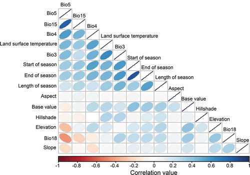
While the variables from the VIF calculation process showed low VIF values, the correlation matrix (Figure 3) revealed further mild correlations (r < 0.7) among some of the variables. The variables correlation matrix of the 14 “VIF-selected” variables using the Pearson correlation coefficient is shown in Figure 3.

Figure 3. Collinearity matrix of the predictors used in this study. Lighter tones of the blue and red colors imply low variable collinearity, while dark shades show high collinearity. The inclination of the ellipse shows a positive or negative correlation

2.7. Species distribution models implementation

The “sdm” package (Naimi and Araújo 2016) performed in R (R Core Team 2020) was used to simulate the SGH habitat suitability and ecological niche. The “sdmdata” function was used to generate 1000 “pseudo-absence” points that were combined with the 125 “presence-only” used in this analysis. These 125 occurrence points were sufficient since Stockwell and Peterson (2002) concluded that predicting the occurrence of a species at a location could be at 90% of maximum prediction accuracy using 10 sample points and could be close to 100% using 50 data points. This suggests that our 125 “presence-only” sample points were sufficient at a national scale. Pseudo-absence points have been used by several other studies since obtaining real “presence-absence data” is logistically impractical (Phillips et al. 2009; Ozdemir et al. 2018). However, like other ecological niche models, “sdm” allows for the use of “presence-only” observations, by generating background “pseudo-absence” data (Naimi and Araújo 2016).

The package “sdm” merges different parallel executions of ecological niche models in a single program using an object-oriented reproducible and extensible framework for ecological niche models in R (Naimi and Araújo 2016). Only 3 of the 15 were used in this study i.e. MaxEnt, RF, and SVM. MaxEnt calculates a conditional probability of occurrence using the density of the covariates at “presence” sites and the marginal density of the covariates in the rest of the study area (Elith et al. 2010). The RF uses a forest of random decision trees and prediction is done by selecting the class with the highest votes (Bangira et al. 2019), while SVM uses a hyperplane to estimate the divergence of class groupings for the prediction (Vapnik 1979). Comparatively, MaxEnt is widely used and reliably better in its predictive performance and usefulness as evidenced by over 1000 ecological applications published since 2006 (Merow, Smith, and Silander 2013; Booth 2018; Booth et al. 2014). Moreover, the aforementioned three machine learning algorithms are efficient in conducting complex species distribution experiments and provide relatively higher modeling accuracies compared to the other methods like boosting (Abdel-Rahman, Ahmed, and Ismail 2013; Mosomtai et al. 2016; Mudereri et al. 2020b; Sarvia, De Petris, and Borgogno-Mondino 2020). A summary of these models’ execution syntax and their corresponding packages used by “sdm” in the parallel model simulations are provided in Table 2.

Table 2. R software packages used by “sdm” in the parallel execution of the three models; namely maximum entropy (MaxEnt), random forest (RF), and support vector machines (SVM)

Algorithm	Syntax code in “sdm”	Package used	Reference
Maximum entropy	“maxent”	dismo	(Phillips, Anderson, and Schapire 2006)
Random forest	“rf”	randomForest	(Liaw, Wiener, and Weiner 2002)
Support vector machines	“svm”	Kernlab	(Karatzoglou et al. 2004)

The future was predicted by only changing the selected climatic variables, but all the other variables were assumed to remain constant in the future. An ensemble projection approach was used to harmonize the variations produced by the different model predictions. Ensemble modeling binds together the highest performance of all the models that have the most acceptable precision and accuracy (Naimi and Araújo 2016). In the current study, the “ensemble” function within the “sdm” package was used to generate the ensemble using the true skill statistic (TSS) weighted average approach (Naimi and Araújo 2016).

The predicted suitable area for the probability of SGH occurrence was calculated using threshold values i.e. ≥ 0.3 for the suitable area, while < 0.3 was regarded as unsuitable (Abdelaal et al. 2019). Using these values, a binary raster image of the suitable versus unsuitable classes for the whole study area was created. Using all the 182 PA boundary shapefile in R, the predicted binary values for each pixel were extracted. The total number of pixels for each predicted class was used to estimate the total coverage of the predicted suitable area against the unsuitable area within and outside of the PAs. For clarity, in this study, we only report on the eleven National parks in Zimbabwe as these are perceived to receive the maximum protection compared to the other PA categories. The final maps for displaying the SGH habitat suitability were developed using QGIS software version 3.10.11 (https://www.qgis.org/en/site/)

2.8. Models’ accuracy validation

A 10-fold cross-validation approach was used for subsampling the data using the inbuilt randomly split “independent test dataset” in the “sdm” package, universally to each of the three models. The 10-fold cross-validation approach was used because it validates the performance of models on multiple folds, which provides a more stable output of how the model performs. Furthermore, since every data point is tested exactly once and is used in the training set k-1 times, it reduces selection bias and flags overfitting of the model. However, if identical samples are present in the dataset it may cause “twinning” since the point will feed identical information into the model. In this study, “twinning” was not experienced because only one sample was kept for each 1 km x 1 km grid (Phillips et al. 2009). The performance of the three models was then measured using the area under the curve (AUC) and TSS (Allouche, Tsoar, and Kadmon 2006) available in the “sdm” package. Generally, an AUC or TSS value of ≥ 0.7 demonstrates high model prediction performance (Tsoar et al. 2007). The McNemar test (Mcnemar 1947) was further used to compare if there were significant differences among the predicted outputs by the three models.

3. Results

3.1. Models’ accuracy, comparison, and validation

The values of the calculated VIF of the predictor variables used in the three models are summarized in Table 1. The most independent variables as shown by the lowest values of VIF were related to terrain variables i.e. aspect (1.14) and hillshade (1.15), while bioclimatic variables had slightly higher values of VIF such as Bio3 (2.32), Bio4 (2.33), Bio18 (5.62) and Bio15 (8.41). These values suggested low collinearity among these variables hence were included in the model. On the other hand, the VIF values for other bioclimatic variables such as Bio11 and Bio8 were 31.62 and 25.04, respectively, and thus were excluded from the final modeling analysis as they were considered not independent (Tables S1 and S2).

Using the receiver operating curve (ROC), results showed that all the models i.e. MaxEnt, RF, and SVM were consistent in their prediction (Figure 4). All the models displayed relatively high accuracy (AUC > 0.87 and TSS > 0.65) in predicting SGH occurrence in Zimbabwe. RF had the highest values of AUC (0.95) and TSS (0.79) while the MaxEnt produced the lowest AUC (0.87) and TSS (0.65) scores (Figure 4). The results also show variations, where models such as the MaxEnt had a higher AUC but lower TSS, demonstrating variation in the specificity and sensitivity of the models.

Figure 4. ROC for the three models used to predict SGH occurrence in Zimbabwe viz. (a) random forest (RF), (b) support vector machines (SVM), and (c) maximum entropy (MaxEnt). The red and blue curves are the mean area under the curve (AUC) using the training and test data, respectively. The light blue curves show the 10-fold replicated model runs using the training data

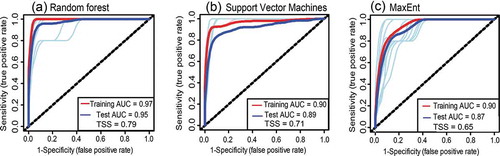
Although the AUC and TSS metrics of the three models showed differences, the McNemar test showed that there were no significant differences (p < 0.001) in the predicted outputs by the three models, indicating that all the three models performed similarly in terms of accuracy (Table 3).

Table 3. McNemar test for comparing the performance of the three machine learning models in predicting the suitable habitat for the SGH. MaxEnt, RF, and SVM are maximum entropy, random forest, and support vector machine models, respectively using the current climate scenario

Models’ comparison	Chi-square	p-value
RF vs MaxEnt	30.02	< 0.001aa
RF vs SVM	10.32	< 0.001aa
SVM vs MaxEnt	9.25	0.001a

a Significant at 95% confidence interval (CI); aa Significant at 99% CI

3.2. Variable importance using the current climate scenario

Of the 14 predictor variables, two (i.e. iso-thermality’ (Bio3) and “temperature seasonality” (Bio4)) were the top five most relevant variables across the three models. The “maximum temperature of the warmest month” (Bio5), “precipitation of warmest quarter” (Bio18), “length of the season” and elevation consistently appeared in the top ten of the most important variables for all the three models. The respective variable contributions of the 14 variables as they appear in the different models are summarized in Figure 5.

Figure 5. Variable importance for predicting SGH occurrence in Zimbabwe using (a) random forest (RF), (b) support vector machines (SVM), and (c) maximum entropy (MaxEnt)

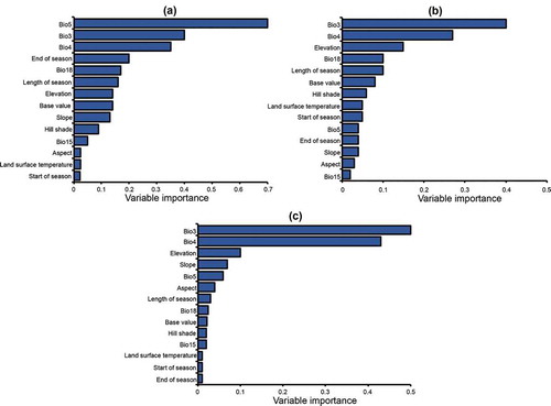
The bioclimatic and seasonality parameters dominated the most relevant variables list while the topographic and LST had low relevance across the three algorithms tested. Topography variables appeared in all the models at different contribution levels; however, elevation appeared more frequently than the other terrain variables. LST appeared once among the ten most important variables for the SVM. RF, which had the highest accuracy (AUC = 0.95) amongst the other models, selected bioclimatic variables i.e. Bio5, Bio3, and Bio4 as the most relevant variables for predicting the occurrence probability of SGH in Zimbabwe (Figure 5).

3.3. The suitable habitat of SGH using the current and future climate scenario within National parks

The three machine learning models using the selected 14 predictor variables demonstrated similar results for the prediction of SGH probability of occurrence (Figure 6). All three models predicted the suitable habitat to be within similar spatial areas although differences in the magnitudes of probabilities were observed among the modeled outputs. The highest prevalence and habitat suitability were predicted in northwestern-based National parks i.e. Hwange, Kazuma pan, Victoria Falls, and Zambezi and their surrounding areas. Furthermore, areas around the Kariba dam and along the Zambezi river were also established as key habitats for the SGH. All these areas occur in the marginal agro-ecological region “V” which is characterized by extensive farming regions suitable for extensive cattle ranching, forestry, wildlife management, and tourism. The lowest suitability was observed in some northern- and eastern-based National parks i.e. Chizarira, Chimanimani, and Nyanga.

Figure 6. SGH habitat suitability under the current and future climate scenarios. The images in a, b, and c show the RF prediction under the current, RCP2.6 (2050) and RCP8.5 (2050) respectively while d, e, and f show the SVM prediction under the current, RCP2.6 (2050) and RCP8.5 (2050), respectively. The MaxEnt prediction under the current, RCP2.6 (2050) and RCP8.5 (2050) is shown by g, h, and i, respectively. The white polygons show the location and boundaries of the main National parks in Zimbabwe

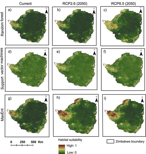
The general trend from the predicted climate changes shows increased potentially suitable habitat for the SGH in most National parks (n = 7) with the largest area being observed under the RCP8.5. However, there were decreases in the suitable habitat in four of the northern- and eastern-based National parks due to the change in climate (Figure 7).

Figure 7. Overall and individual percentage cover of predicted suitable habitat for the SGH within the 11 National parks in Zimbabwe, using the current and future climate scenarios i.e. representative concentration pathway (RCP2.6) and RCP8.5 for the year 2050

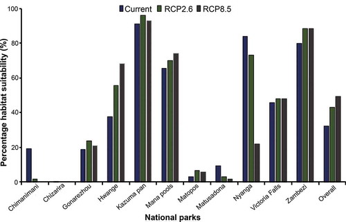
Although the percentage contributions in Figure 7 show that Kazuma pan, Zambezi, and Mana pools were among the top suitable habitat contributors, they, however, have relatively low spatial coverage compared to Hwange and Gonarezhou (Table 4). Also, Table 4 shows that Hwange National park, which is the largest among the National parks in Zimbabwe contributes the most suitable habitat (946.2 km² under current climate) of the SGH while Chimanimani (3.3 km² under current climate) and Chizarira (3.6 km² under current climate) contribute the least. Overall, there is a positive increase in the suitable habitat of between ~ 11% and 17% within the National parks’ category of PAs between the years 2000 and 2050.

Table 4. The total area coverage (km²) and the predicted suitable habitat area (km²) of the SGH within the 11 National parks in Zimbabwe, using the current and future climate scenarios i.e. representative concentration pathway (RCP2.6) and RCP8.5 for the year 2050

National Park	Total area (km^2)	Current (km^2)	RCP2.6 (km^2)	RCP8.5 (km^2)
Chimanimani	171.1	3.3	3.3	0.5
Chizarira	1910	3.6	0.0	0.2
Gonarezhou	5053	946.2	1201.2	1064.6
Hwange	14,651	5489.8	8148.5	9986.1
Kazuma Pan	313	284.6	301.2	290.5
Mana Pools	2196	1437.6	1540.0	1622.7
Matopos	424	13.2	29.3	24.7
Matusadona	1407	134.2	40.8	24.3
Nyanga	330	276.5	241.6	72.0
Victoria Falls	23.4	10.7	11.2	11.2
Zambezi	560	448.5	495.3	495.3
Overall	27,038.5	8714.0	11,681.3	13,336.2

3.4 Suitable habitat for the SGH under current and future climate scenarios in different PA categories

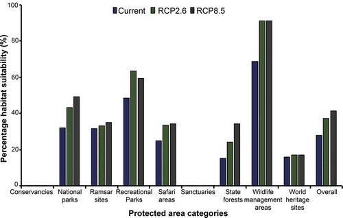
Results show that the various “Wildlife Management Areas” across the country have the highest percentage (> 90%) of the suitable habitat followed by recreational areas (± 60%) and National parks (50%). However, this does not relate to the spatial coverage across the different categories but within the boundary of the specific category (intra-category). Conservancies and sanctuaries have the least or no area suitable for the SGH probably because of their location and not necessarily on their protection status or management effectiveness. Overall, an increase (~10%) in suitability across the different categories of PAs is projected under climate change (Figure 8).

Figure 8. Overall and individual habitat suitability area percentage cover in 9 categories of protected areas in Zimbabwe, using the current and future climate scenario i.e. representative concentration pathway (RCP2.6) and RCP8.5 for the year 2050

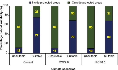
Figure 9 shows the relative proportion of the suitable areas within and outside of the PAs using the current and future climate scenario i.e. RCP2.6 and RCP8.5 for the year 2050. Results show a decline in the proportion of the suitable area within PAs toward unprotected areas. In general, there is a decline from 77% of the suitable area under the current climate to 69% under RCP8.5 (2050). Conversely, there is a gain (8%) in suitability outside of the PAs network from 23% to 31%. These results demonstrate that when the analysis is performed within the PAs network without considering the unprotected areas, PAs generally show gains in suitable habitat while when compared with the unprotected areas at the country level they show a slight decline (~8%) for both scenarios.

Figure 9. Relative proportion of suitable area within and outside PAs using the current and future climate scenarios i.e. representative concentration pathway (RCP2.6) and RCP8.5 for the year 2050

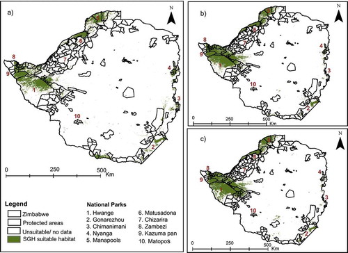
The results of the ensemble projection of the three models using the current (1970–2000) and future (2050) climate scenario combined the best predictions of all the models and estimated the overall SGH habitat suitability to be mostly within PAs with few areas outside the PAs network (Figure 10). The spatial analysis shown in Figure 10 shows, interestingly, that the three models concur that habitat suitability of SGH is high along the eastern, northern, and western borders of the country with less suitability in the inner central areas of the country. Further, the western areas have large swaths suitable for SGH in Zimbabwe compared to other areas (Figure 10).

Figure 10. Predicted SGH suitable habitat from ensemble projection and weighted average of true skill statistic (TSS) of the three models, viz. maximum entropy (MaxEnt) random forest (RF), and support vector machines (SVM) under (a) current, (b) RCP2.6, and (c) RCP8.5

4. Discussion

In this study, threemachine learning models were used to simulate the current SGH probability habitat suitability in Zimbabwe. The quality of the predictor variables, response variables, model evaluation ideals were examined while building multiple models using the same input data was applied before the actual modeling procedure following the protocols suggested by Araújo et al. (2019). The three machine learning models were employed to test the hypothesis that PAs would be more effective at preserving and maintaining the SGH habitat than unprotected areas. By quantifying the change in modeled habitat suitability over different climatic regimes, instead of the direct changes in species abundance, we examined whether suitable SGH habitat persisted within PAs than the unprotected areas (Lecina-Diaz et al. 2019). The assumption was that the mechanism central to the effectiveness of PAs is the extent to which they protect and ensure the resilience of suitable habitat (McCune, Van Natto, and MacDougall 2017).

The three predictive models showed relatively high predictive power i.e. AUC and TSS values larger than 0.8 and 0.65 respectively suggesting a plausible simulation performance (Tsoar et al. 2007). Our results identified RF as the best predictive model, confirming the robustness of the RF model in predicting simulation outcomes with multi-source covariates reported in other studies (Hallman and Robinson 2020; Kampichler et al. 2010; Mudereri et al. 2020b). Although they produce similar results, the three models show relatively different outputs, which was expected as they use different equations and approaches to perform the prediction hence the ensemble model (Naimi and Araújo 2016). Nonetheless, the bioclimatic conditions spatially demonstrated by the three models have been inferred as a proxy measure representing the general magnitude of change within the landscape occupied or potential habitat for SGH.

The finding that demonstrates the longer-term variables such as “iso-thermality” (Bio3) and “temperature seasonality” (Bio4) are more important compared to specific time window variables is explained by the fact that the breeding season for SGH can be as long as eight months with nests used for successive years (Msimanga 2004) and thus suitable conditions are required for a longer period. Also, Kemp and Begg (1996) suggested that nesting sites are more important for SGH habitats than foraging influences and therefore the identified factors are more related to the distribution of the factors associated with nesting of the SGH.

Our prior assumptions and hypothesis were confirmed as our analysis demonstrated that the major portion of the suitable habitat for the SGH is currently within PAs and shall increase and remain within PAs under climate change. Several studies reiterate this huge reliance of the SGH on the PAs for its survival (Broms et al. 2014; Combrink et al. 2017; Kemp, Benn, and Begg 1998; Witteveen et al. 2013), however, none had established environmental tolerance of the SGH using future climate scenarios. The observed current and future dependence on the PAs by the SGH could be attributed to the vast availability of feed, reduced disturbance of their preferred savanna grasslands, and availability of forest areas for breeding (Witteveen et al. 2013). There is, however, a high probability of substantial continuing impact on the ecological stability within the present protected area network in Zimbabwe, with the majority of the PAs facing extensive ecosystem and species changes or spatial shifts and novel bioclimatic conditions by 2050 (Zomer et al. 2015; Lecina-Diaz et al. 2019; Thamaga and Dube 2019). Thus, there is a great need to regularly monitor suitable habitat for the SGH particularly ensuring availability and maintenance of large trees necessary for nesting and breeding of the SGH.

Additionally, the dynamics of predicting specific vegetation cover types that influence habitat preference indicators (e.g. presence of foraging and nest building resources) of the SGH are challenging when using purely bioclimatic or ecophysiological variables such as those used in this study (Hallman and Douglas Robinson 2020; McCune, Van Natto, and MacDougall 2017). This is mainly because of other secondary factors introduced by climate-induced ecological perturbance such as food availability, deforestation, bush encroachment, natural disasters and, the response and resilience of the protected area management system (Zomer et al. 2015; McCune, Van Natto, and MacDougall 2017). However, temperature and precipitation tolerances, as evidenced in this study, define the potential range of most ecosystems and species particularly large carnivorous birds such as the SGH (Combrink et al. 2017). Moreover, in this study, the comprehensive seasonality parameters that capture the vegetation greenness using the EVI as a proxy for the vegetation type and density preferred by the SGH were used, thus vindicating the results of this study. However, further studies that establish the sufficiency and availability of nesting sites in Zimbabwe are necessary.

Although the bioclimatic conditions under the different climate scenarios tested in this study seem to favor the SGH as shown by the potential increase in habitat suitability, the ability to survive, adapt or benefit from these changes is site-specific and depends on factors such as population dynamics, frequency of drought occurrences, availability of feed, habitat fragmentation, the permeability of the landscape matrix, and physiological adaptability (Eklund et al. 2016; Poor et al. 2019; Guerra, Rosa, and Pereira 2019). If the ecophysiological conditions within PAs proceed beyond those conducive for the SGH, or if invasive and competitive species are introduced, the conservation effectiveness of these PAs will considerably decrease (Zomer et al. 2015). Therefore, although the habitat for the SGH will remain relatively stable, regular monitoring against the chances of invasive species, desertification, and loss of nesting sites is necessary and highly recommended within and outside of the PAs network.

This study established that the habitat would remain relatively suitable in the western-based areas compared to the eastern regions. This can be attributed to the differences in the altitude of these two regions (Bandopadhyay 2016). The eastern region is mainly characterized by high altitude mountains and hills while the western regions are low-lying (Mugandani et al. 2012). Studies have projected that high altitude regions are likely to warm at a faster rate than the lower elevation areas (Bandopadhyay 2016; Niang et al. 2014). This leads to the widening of the gap between the maximum and minimum temperatures compared to low-lying areas hence higher probabilities of the loss of suitable habitat for the SGH in the eastern regions.

This study also established that an increase in habitat suitability outside of the PAs network in Zimbabwe is likely with an 8% gain in suitability. These results concur with the study of Witteveen et al. (2013) who established successful nesting and breeding of the SGH in communal areas surrounding Matopos National park. The study identified positive human-SGH coexistence and availability of abundant feed under communal farming conditions as some of the major factors increasing habitat suitability outside PAs. Such hybrid conservation efforts may, therefore, become more important under projected climate conditions as habitats outside the traditional PAs will have increased suitability for SGH. However, it is not known whether the increase in the suitable habitat outside the PAs network (from 23% to 31%) may eventually cause conflicts between conservation and agricultural objectives of local communities. To resolve these potential conflicts, we suggest improved cross-boundary collaboration and policy development among involved institutional structures, combined with stakeholder participation to implement a holistic conservation plan. This is even more necessary given that the suitable habitats for SGH are in national border areas with neighboring countries. Besides, the modeled effects of climate change on SGH suitability come in addition to other threats such as mercury (Daso et al. 2015) and lead (Koeppel and Kemp 2015) poisoning in the region.

Further, the analysis established that the different categories of PAs will have different levels of suitable habitat under climate change. Higher levels of protection resulted in higher levels of suitable habitat for the SGH. It is thus paramount to enhance their security as other studies have suggested that PAs are failing to maintain the exploitation of biological components within them (Lecina-Diaz et al. 2019). The “Wildlife Management Areas” category was identified as one of the key areas to house the SGH. However, most of these areas are privately owned and property owners would require awareness on strategies of maintaining the SGH habitat and safeguarding breeding sites within individual landholdings (McCune, Van Natto, and MacDougall 2017). It was however interesting to note that the network of PAs in the western and northwestern regions provided a continuous and interwoven potential habitat for the SGH. Hwange, Kazuma Pan, Victoria Falls, and Zambezi National parks were confirmed by this study as the hubs and fundamental reservoirs of potentially suitable habitat for the SGH. Thus, these should be monitored consistently.

4.1. Limitations of the study

Our study categorized all the 182 PAs (Figure 2) in one class and all the areas outside of these legally recognized areas as unprotected. For all the PAs in Zimbabwe, the nature of activities and security varies for both inter- and intra-protection categories, as such influences the level of strictness, the animal species diversity and abundance. For instance, some areas are more protected than the National parks regarding management and security e.g. Malilangwe, Save Valley, and Bubi. Therefore, our results may be used with caution as regards such privately owned PAs. However, as the management practices differ from one PA to the other, it remains a challenge to factor the individual quality of management of all the 182 PAs in Zimbabwe within this study.

Moreover, there was no available information on specific tree species that SGH prefers for nesting, therefore vegetation phenological variables were used as indicators for nesting. On the other hand, the 10-fold cross-validation approach was used in this study instead of using an independent dataset to robustly validate the SGH habitat suitability models. One of the limitations of this validation approach is that it aggregates the validation scores across the 10 folds, which might not give reliable information on the stability of the model performance if the data are not well distributed across the folds.

Conclusions

The results of the present study suggest that the current PAs network in Zimbabwe, particularly in the western and north-western regions provide a potentially suitable habitat to conserve SGH. Furthermore, the Kariba-Zambezi river region comprising of the Hwange, Kazuma Pan, Victoria Falls, and Zambezi National parks are strategic and key priority areas for the conservation of SGH. Although the lowest-ranked conservation areas are mostly found in the eastern region of the country, the habitats in these regions must be protected to ensure safe hubs for the SGH in the face of climate change. It would also be more prudent to educate and sensitize the private owners of the wildlife management areas on the importance of maintaining pristine habitat areas for the SGH. Also, maintaining a design of a large PA network such as observed around Hwange National park with a wide geographical, grassland, and forest extents are likely to provide a better buffer to the effects of range shifts in species and community distributions as a result of climate change. We, however, note that our dataset only covers a small portion of the SGH distribution in Africa. Therefore, our conclusions on the species habitat associations and potentially suitable habitat are limited to Zimbabwe. Further analyses should be conducted to determine if the relationships hold for the rest of its range e.g. in Botswana, Mozambique, South Africa, Zambia, Namibia, Tanzania, Democratic Republic of Congo, and Kenya.

Highlights

• We developed ecological suitability models for the Southern Ground-hornbill (SGH)

• Suitable habitat was matched with protected areas (PAs) coverage.

• PAs are extremely relevant for the SGH habitat preservation

• Western PAs will increase in suitable habitat while eastern-based will decrease

Acknowledgements

We gratefully acknowledge the financial support for this research by the following organizations and agencies: UK’s Foreign, Commonwealth & Development Office (FCDO); Swedish International Development Cooperation Agency (Sida); the Swiss Agency for Development and Cooperation (SDC); Ethiopian and Kenyan Governments. ‘B.T.M’ was supported by a German Academic Exchange Service (DAAD) In-Region Postgraduate Scholarship. The views expressed herein do not necessarily reflect the official opinion of the donors.

Data availability statement

The data that support the findings of this study are available in GBIF at https://www.gbif.org, reference number 10.15468/dl.lby4qk. These data were derived from the following resources available in the public domain: doi.org/10.15468/dl.lby4qk

Disclosure statement

The authors declare no conflict of interest.

Supplementary material

Supplemental data for this article can be accessed here.

References

- Abdelaal, M., M. Fois, G. Fenu, and G. Bacchetta. 2019. “Using MaxEnt Modeling to Predict the Potential Distribution of the Endemic Plant Rosa Arabica Crép. In Egypt.” Ecological Informatics 50: 68–75. doi:10.1016/j.ecoinf.2019.01.003.
- Abdel-Rahman, E. M., F. B. Ahmed, and R. Ismail. 2013. “Random Forest Regression and Spectral Band Selection for Estimating Sugarcane Leaf Nitrogen Concentration Using EO-1 Hyperion Hyperspectral Data.” International Journal of Remote Sensing 34 (2): 712–728. doi:10.1080/01431161.2012.713142.
- Allouche, O., A. Tsoar, and R. Kadmon. 2006. “Assessing the Accuracy of Species Distribution Models: Prevalence, Kappa and the True Skill Statistic (TSS).” Journal of Applied Ecology 43 (6): 1223–1232. doi:10.1111/j.1365-2664.2006.01214.x.
- Araujo, M. B., R. G. Pearson, W. Thuiller, and M. Erhard. 2005. “Validation of Species-Climate Impact Models under Climate Change.” Global Change Biology 11 (9): 1504–1513. doi:10.1111/j.1365-2486.2005.001000.x.
- Araújo, M. B., R. P. Anderson, M. A. Barbosa, C. M. Beale, C. F. Dormann, R. Early, R. A. Garcia, et al. 2019. “Standards for Distribution Models in Biodiversity Assessments.” Science Advances 5 (1): 1–12. doi:10.1126/sciadv.aat4858.
- Bandopadhyay, S. 2016. “Does Elevation Impact Local Level Climate Change? an Analysis Based on Fifteen Years of Daily Diurnal Data and Time Series Forecasts.” Pacific Science Review A: Natural Science and Engineering 18 (3): 241–253. doi:10.1016/j.psra.2016.11.002. Elsevier Ltd.
- Bangira, T., A. Van Niekerk, M. Menenti, and S. M. Alfieri. 2019. “Comparing Thresholding with Machine Learning Classifiers for Mapping Complex Water.” Remote Sensing 1–21. doi:10.3390/rs11111351.
- BirdLife International. 2020. “Species Fact Sheet: Bucorvus Leadbeateri Downloaded from Http://Www,Birdlife.Org on 27 03 2020.”
- Booth, T. H. 2018. “Why Understanding the Pioneering and Continuing Contributions of BIOCLIM to Species Distribution Modelling Is Important.” Austral Ecology 43 (8): 852–860. doi:10.1111/aec.12628.
- Booth, T. H., H. A. Nix, J. R. Busby, and M. F. Hutchinson. 2014. “Bioclim: The First Species Distribution Modelling Package, Its Early Applications and Relevance to Most Current MaxEnt Studies.” Diversity & Distributions 20 (1): 1–9. doi:10.1111/ddi.12144.
- Breiman, L. 2001. “Random Forests.” Machine Learning 45: 5–32. doi:10.1023/A:1010933404324.
- Broms, K. M., D. S. Johnson, R. Altwegg, and L. L. Conquest. 2014. “Spatial Occupancy Models Applied to Atlas Data Show Southern Ground Hornbills Strongly Depend on Protected Areas.” Ecological Applications. doi:10.1890/12-2151.1.
- CGIAR-CSI. 2019. “SRTM.” http://srtm.csi.cgiar.org/.
- Chiweshe, N. 2007. “The Current Conservation Status of the Southern Ground Hornbill Bucorvus Leadbeateri in Zimbabwe.” Proceedings of the 4th International Hornbill Conference: The Active Management of Hornbills and Habitats for Conservation 4–9 November 2005, Bela Bela, 252–266.
- Combrink, L., H. J. Combrink, A. J. Botha, and C. T. Downs. 2017. “Nest Temperature Fluctuations in a Cavity Nester, the Southern Ground-Hornbill.” Journal of Thermal Biology. doi:10.1016/j.jtherbio.2017.03.003.
- Core Team, R. 2020. “R: A Language and Environment for Statistical Computing. R Foundation for Statistical Computing, Vienna, Austria. Https://Www.R-Project.Org/.” Vienna, Austria.
- Daso, A. P., J. O. Okonkwo, R. Jansen, J. D. D. O. Brandao, and A. Kotzé. 2015. “Mercury Concentrations in Eggshells of the Southern Ground-Hornbill (Bucorvus Leadbeateri) and Wattled Crane (Bugeranus Carunculatus) in South Africa.” Ecotoxicology and Environmental Safety 114. Elsevier: 61–66. doi:10.1016/j.ecoenv.2015.01.010.
- Development Team, Q. G. I. S. 2019. “QGIS Geographic Information System.” Open Source Geospatial Foundation Project Http://qgis.osgeo.org
- Dormann, C. F., J. Elith, S. Bacher, C. Buchmann, G. Carl, G. Carré, R. Jaime, et al. 2013. “Collinearity: A Review of Methods to Deal with It and A Simulation Study Evaluating Their Performance.” Ecography 36 (1): 027–046. doi:10.1111/j.1600-0587.2012.07348.x.
- Eklund, J. F., G. Blanchet, J. Nyman, R. Rocha, T. Virtanen, and M. Cabeza. 2016. “Contrasting Spatial and Temporal Trends of Protected Area Effectiveness in Mitigating Deforestation in Madagascar.” Biological Conservation 203. Elsevier B.V.: 290–297. doi:10.1016/j.biocon.2016.09.033.
- Eklundh, L., and J. Per. 2017. TIMESAT 3.3 With Seasonal Trend Decomposition and Parallel Processing Software Manual, 1–92. Sweden: Lund and Malmo University.
- Elith, J., T. Hastie, M. Dudík, Y. E. Chee, C. J. Yates, and S. J. Phillips. 2010. “A Statistical Explanation of MaxEnt for Ecologists.” Diversity & Distributions 17 (1): 43–57. doi:10.1111/j.1472-4642.2010.00725.x.
- Feng, Y., Y. Liu, and X. Tong. 2018. “Spatiotemporal Variation of Landscape Patterns and Their Spatial Determinants in Shanghai, China.” Ecological Indicators 87 (July 2017). Elsevier: 22–32. doi:10.1016/j.ecolind.2017.12.034.
- Fick, S. E., and R. J. Hijmans. 2017. “WorldClim 2: New 1-Km Spatial Resolution Climate Surfaces for Global Land Areas.” International Journal of Climatology 37 (12): 4302–4315. doi:10.1002/joc.5086.
- Gandiwa, E., T. Magwati, P. Zisadza, T. Chinuwo, and C. Tafangenyasha. 2011. “The Impact of African Elephants on Acacia Tortilis Woodland in Northern Gonarezhou National Park, Zimbabwe.” Journal of Arid Environments 75 (9): 809–814. doi:10.1016/j.jaridenv.2011.04.017. Elsevier Ltd.
- GBIF. 2019. “GBIF Occurrence Download.” doi:10.15468/dl.lby4qk.
- Gong, M., Z. Fan, X. Zhang, G. Liu, W. Wen, and L. Zhang. 2017. “Measuring the Effectiveness of Protected Area Management by Comparing Habitat Utilization and Threat Dynamics.” Biological Conservation 210 (April): 253–260. doi:10.1016/j.biocon.2017.04.027.
- Guerra, C. A., I. M. D. Rosa, and H. M. Pereira. 2019. “Change versus Stability: Are Protected Areas Particularly Pressured by Global Land Cover Change?” Landscape Ecology 34 (12): 2779–2790. doi:10.1007/s10980-019-00918-4.
- Hallman, T. A., and W. Douglas Robinson. 2020. “Comparing Multi- and Single-Scale Species Distribution and Abundance Models Built with the Boosted Regression Tree Algorithm.” Landscape Ecology 7. doi:10.1007/s10980-020-01007-7.
- Hentze, K., F. Thonfeld, and G. Menz. 2016. “Evaluating Crop Area Mapping from Modis Time-Series as an Assessment Tool for Zimbabwe’s ‘Fast Track Land Reform Programme’.” PLoS ONE 11 (6): 1–22. doi:10.1371/journal.pone.0156630.
- IPCC. 2014. Climate Change 2014: Synthesis Report. Contribution of Working Groups I, II and III to the Fifth Assessment Report of the Intergovernmental Panel on Climate Change. Ipcc.
- Kampichler, C., R. Wieland, S. Calmé, H. Weissenberger, and S. Arriaga-Weiss. 2010. “Classification in Conservation Biology: A Comparison of Five Machine-Learning Methods.” Ecological Informatics 5 (6): 441–450. doi:10.1016/j.ecoinf.2010.06.003.
- Karatzoglou, A., A. Smola, K. Hornik, and A. Zeileis. 2004. “Kenlab - an S4 Package for Kernel Methods in R.” Journal of Statistical Software 11 (9): 1–20. http://www/jstatsoft.org/v11/i09/.
- Kemp, A. C., G. A. Benn, and K. S. Begg. 1998. “Geographical Analysis of Vegetation Structure and Sightings for Four Large Bird Species in the Kruger National Park, South Africa.” Bird Conservation International. doi:10.1017/S0959270900003658.
- Kemp, A. C., and K. S. Begg. 1996. “Nest Sites of the Southern Ground Hornbill Bucorvus Leadbeateri in the Kruger National Park, South Africa, and Conservation Implications.” Ostrich 67 (1): 9–14. doi:10.1080/00306525.1996.9633773.
- Koeppel, K. N., and L. V. Kemp. 2015. “Lead Toxicosis in a Southern Ground Hornbill Bucorvus Leadbeateri in South Africa.” Journal of Avian Medicine and Surgery 29 (4): 340–344. doi:10.1647/2014-037.
- Kyalo, R., E. Abdel-Rahman, S. Mohamed, S. Ekesi, B. Christian, and T. Landmann. 2018. “Importance of Remotely-Sensed Vegetation Variables for Predicting the Spatial Distribution of African Citrus Triozid (Trioza Erytreae) in Kenya.” ISPRS International Journal of Geo-Information 7 (11): 429. doi:10.3390/ijgi7110429.
- Kyalo, R., E. M. Abdel-Rahman, J. O. Sevgan Subramanian, M. T. Nyasani, H. Jozani, C. Borgemeister, and T. Landmann. 2017. “Maize Cropping Systems Mapping Using RapidEye Observations in Agro-Ecological Landscapes in Kenya.” Sensors 17 (11): 2537. doi:10.3390/s17112537.
- Kylin, H., H. Bouwman, and S. W. Evans. 2011. “Evaluating Threats to an Endangered Species by Proxy: Air Pollution as Threat to the Blue Swallow (Hirundo Atrocaerulea) in South Africa.” Environmental Science and Pollution Research 18 (2): 282–290. doi:10.1007/s11356-010-0369-0.
- Lecina-Diaz, J., A. Alvarez, M. De Cáceres, S. Herrando, J. Vayreda, and J. Retana. 2019. “Are Protected Areas Preserving Ecosystem Services and Biodiversity? Insights from Mediterranean Forests and Shrublands.” Landscape Ecology 34 (10): 2307–2321. doi:10.1007/s10980-019-00887-8.
- Liaw, A., M. Wiener, and M. Weiner. 2002. “Classification and Regression by RandomForest.” R News 2 (3): 18–22. doi:10.1177/154405910408300516.
- Manish, K., and M. K. Pandit. 2019. “Identifying Conservation Priorities for Plant Species in the Himalaya in Current and Future Climates: A Case Study from Sikkim Himalaya, India.” Biological Conservation 233 (February): 176–184. doi:10.1016/j.biocon.2019.02.036. Elsevier.
- McCarthy, J. K., J. M. Dwyer, and K. Mokany. 2020. “Direct Climate Effects are More Influential than Functional Composition in Determining Future Gross Primary Productivity.” Landscape Ecology 0123456789. Springer Netherlands. doi:10.1007/s10980-020-00994-x.
- McCune, J. L., A. Van Natto, and A. S. MacDougall. 2017. “The Efficacy of Protected Areas and Private Land for Plant Conservation in a Fragmented Landscape.” Landscape Ecology 32 (4): 871–882. doi:10.1007/s10980-017-0491-1. Springer Netherlands.
- Mcnemar, Q. 1947. “Note on the Sampling Error of the Difference between Correlated Proportions or Percentages.” Psychometrika 12 (2): 153–157. doi:10.1007/BF02295996.
- Merow, C., M. J. Smith, and J. A. Silander. 2013. “A Practical Guide to MaxEnt for Modeling Species’ Distributions: What It Does, and Why Inputs and Settings Matter.” Ecography 36 (10): 1058–1069. doi:10.1111/j.1600-0587.2013.07872.x.
- Moreno, R., R. Zamora, J. R. Molina, A. Vasquez, and M. Á. Herrera. 2011. “Predictive Modeling of Microhabitats for Endemic Birds in South Chilean Temperate Forests Using Maximum Entropy (Maxent).” Ecological Informatics 6 (6): 364–370. doi:10.1016/j.ecoinf.2011.07.003.
- Mosomtai, G., M. Evander, P. Sandström, C. Ahlm, R. Sang, O. A. Hassan, H. Affognon, and T. Landmann. 2016. “Association of Ecological Factors with Rift Valley Fever Occurrence and Mapping of Risk Zones in Kenya.” International Journal of Infectious Diseases 46: 49–55. doi:10.1016/j.ijid.2016.03.013.
- Msimanga, A. 2004. “Breeding Biology of Southern Ground Hornbill Bucorvus Leadbeateri in Zimbabwe: Impacts of Human Activities.” Bird Conservation International. doi:10.1017/S0959270905000237.
- Mudereri, B. T., C. Mukanga, E. T. Mupfiga, C. Gwatirisa, E. Kimathi, and T. Chitata. 2020a. “Analysis of Potentially Suitable Habitat within Migration Connections of an Intra-African Migrant-the Blue Swallow (Hirundo Atrocaerulea).” Ecological Informatics 57: 101082. doi:10.1016/j.ecoinf.2020.101082.
- Mudereri, B. T., E. M. Abdel-Rahman, T. Dube, T. Landmann, Z. Khan, E. Kimathi, R. Owino, and S. Niassy. 2020b. “Multi-Source Spatial Data-Based Invasion Risk Modeling of Striga (Striga Asiatica) in Zimbabwe.” GIScience and Remote Sensing 57 (4): 553–571. doi:10.1080/15481603.2020.1744250.
- Mugandani, R., M. Wuta, A. Makarau, and B. Chipindu. 2012. “RE-Classification of Agro-Ecological Regions of Zimbabwe in Conformity with Climate Variability and Change.” African Crop Science Journal 20 (2): 361–369. https://pdfs.semanticscholar.org/d24a/4e02f534cf8e9f8705690c7a5ba19145becc.pdf.
- Muposhi, V. K., E. Gandiwa, A. Chemura, P. Bartels, S. M. Makuza, and T. H. Madiri. 2016. “Habitat Heterogeneity Variably Influences Habitat Selection by Wild Herbivores in a Semi-Arid Tropical Savanna Ecosystem.” PLoS ONE 11: 9. doi:10.1371/journal.pone.0163084.
- Naimi, B., and M. B. Araújo. 2016. “Sdm: A Reproducible and Extensible R Platform for Species Distribution Modelling.” Ecography 39 (4): 368–375. doi:10.1111/ecog.01881.
- Niang, I., O. C. Ruppel, M. A. Abdrabo, A. Essel, C. Lennard, J. Padgham, and P. Urquhart. 2014. “Africa.”In Climate Change 2014: Impacts, Adaptation, and Vulnerability. Part B: Regional Aspects. Contribution of Working Group II to the Fifth Assessment Report of the Intergovernmental Panel on Climate Change [Barros, edited by V. R. Barros, C. B. Field, D. J. Dokken, M. D. Mastrandrea, K. J. Mach, T. E. Bilir, M. Chatterjee, et al., 1199–1265. edited by and L.L. White. Cambridge, United Kingdom and New York, NY, USA: Cambridge University Press. doi:10.1017/CBO9781107415386.002.
- Nyakarahuka, L., S. Ayebare, G. Mosomtai, C. Kankya, J. Lutwama, F. N. Mwiine, and E. Skjerve. 2017. ““Ecological Niche Modeling for Filoviruses: A Risk Map for Ebola and Marburg Virus Disease Outbreaks in Uganda.”.” PLOS Currents Outbreaks 9: 1–24. doi:10.1371/currents.outbreaks.07992a87522e1f229c7cb023270a2af1.
- O’Donnell, M. S., and D. A. Ignizio. 2012. “Bioclimatic Predictors for Supporting Ecological Applications in the Conterminous United States.” US Geological Survey Data Series 691: 10.
- Ozdemir, I., A. Mert, U. Y. Ozkan, S. Aksan, and Y. Unal. 2018. “Predicting Bird Species Richness and Micro-Habitat Diversity Using Satellite Data.” Forest Ecology and Management 424: 483–493. doi:10.1016/j.foreco.2018.05.030.
- Phillips, S. J., M. Dudík, C. H. Jane Elith, A. L. Graham, J. Leathwick, and S. Ferrier. 2009. “Sample Selection Bias and Presence-Only Distribution Models: Implications for Background and Pseudo-Absence Data.” Ecological Applications 19 (1): 181–197. doi:10.1890/07-2153.1.
- Phillips, S. J., R. P. Anderson, and R. E. Schapire. 2006. “Maximum Entropy Modeling of Species Geographic Distributions.” Ecological Modelling 190 (3–4): 231–259. doi:10.1016/j.ecolmodel.2005.03.026.
- Poor, E. E., E. Frimpong, M. A. Imron, and M. J. Kelly. 2019. “Protected Area Effectiveness in A Sea of Palm Oil: A Sumatran Case Study.” Biological Conservation 234: 123–130. doi:10.1016/j.biocon.2019.03.018.
- Qi, P., C. Zhao, and Z. Feng. 2010. “GIS- and Machine Learning-Based Modeling of the Potential Distribution of Broadleaved Deciduous Forest in the Chinese Loess Plateau.” GIScience and Remote Sensing 47 (1): 99–114. doi:10.2747/1548-1603.47.1.99.
- Sarvia, F., S. De Petris, and E. Borgogno-Mondino. 2020. “Multi-Scale Remote Sensing to Support Insurance Policies in Agriculture: From Mid-Term to Instantaneous Deductions.” GIScience and Remote Sensing. 1–15. doi:10.1080/15481603.2020.1798600.
- Stockwell, D. R. B., and A. Townsend Peterson. 2002. “Effects of Sample Size on Accuracy of Species Distribution Models.” Ecological Modelling 148 (1): 1–13. doi:10.1016/S0304-3800(01)00388-X.
- Thamaga, K. H., and T. Dube. 2019. “Understanding Seasonal Dynamics of Invasive Water Hyacinth (Eichhornia Crassipes) in the Greater Letaba River System Using Sentinel-2 Satellite Data.” GIScience and Remote Sensing 56 (8): 1355–1377. doi:10.1080/15481603.2019.1646988.
- Trail, P. W. 2007. “African Hornbills: Keystone Species Threatened by Habitat Loss, Hunting and International Trade.” Ostrich 78 (3): 609–613. doi:10.2989/OSTRICH.2007.78.3.7.318.
- Tsoar, A., O. Allouche, O. Steinitz, D. Rotem, and R. Kadmon. 2007. “A Comparative Evaluation of Presence-Only Methods for Modelling Species Distribution.” Diversity & Distributions 13 (4): 397–405. doi:10.1111/j.1472-4642.2007.00346.x.
- UNEP-WCMC, and IUCN. 2016. Protected Planet Report 2016. Cambridge, United Kingdom and Gland Switzeland. https://www.iucn.org/theme/protected-areas/our-work/quality-and-effectiveness/world-database-protected-areas-wdpa.
- Valeix, M., H. Fritz, R. Sabatier, F. Murindagomo, D. Cumming, and P. Duncan. 2011. “Elephant-Induced Structural Changes in the Vegetation and Habitat Selection by Large Herbivores in an African Savanna.” Biological Conservation 144 (2): 902–912. doi:10.1016/j.biocon.2010.10.029.
- Vapnik, V. 1979. Estimation of Dependences Based on Empirical Data. Vol. 27. 5165–5184. Nauka, Moscow Translation:Springer Verlag, New York, 1982.
- Wakelin, J., C. G. Oellermann, C. T. Amy-Leigh Wilson, and T. H. Downs. 2018. “Habitat Use by the Critically Endangered Blue Swallow in KwaZulu-Natal, South Africa.” Bothalia 48: 1. doi:10.4102/abc.v48i1.2173.
- Walther, B. A., and V. N. Adriaan. 2015. “Effects of Climate Change on Species Turnover and Body Mass Frequency Distributions of South African Bird Communities.” African Journal of Ecology 53 (1): 25–35. doi:10.1111/aje.12143.
- Wan, Z., S. Hook, and G. Hulley. 2015. “MOD11C2 MODIS/Terra Land Surface Temperature/Emissivity 8-Day L3 Global 0.05Deg CMG V006 [Data Set].” NASA EOSDIS Land Processes DAAC: doi: 10.5067/MODIS/MOD11C2.006.
- Wang, R., L. Qing, H. Shisong, Y. Liu, M. Wang, and G. Jiang. 2018. “Modeling and Mapping the Current and Future Distribution of Pseudomonas Syringae Pv. Actinidiae under Climate Change in China.” PLoS ONE 13 (2): 1–21. doi:10.1371/journal.pone.0192153.
- Witteveen, M., E. Parry, M. Norris-Rogers, and M. Brown. 2013. “Breeding Density of the Southern Ground Hornbill, Bucorvus Leadbeateri, in the Communal Areas Surrounding the Matobo National Park, Zimbabwe.” African Zoology. doi:10.3377/004.048.0226.
- Zhang, Z., X. Shengyong, C. Capinha, R. Weterings, and T. Gao. 2019. “Using Species Distribution Model to Predict the Impact of Climate Change on the Potential Distribution of Japanese Whiting Sillago Japonica.” Ecological Indicators 104: 333–340. doi:10.1016/j.ecolind.2019.05.023.
- Zomer, R. J., X. Jianchu, M. Wang, A. Trabucco, and L. Zhuoqing. 2015. “Projected Impact of Climate Change on the Effectiveness of the Existing Protected Area Network for Biodiversity Conservation within Yunnan Province, China.” Biological Conservation 184: 335–345. doi:10.1016/j.biocon.2015.01.031.
- Zoungrana, B. J. B., C. Conrad, L. K. Amekudzi, M. Thiel, and D. E. Dapola. 2015. “Land Use/cover Response to Rainfall Variability: A Comparing Analysis between NDVI and EVI in the Southwest of Burkina Faso.” Climate 3: 63–77. doi:10.3390/cli3010063.