Retrieval of daily sea ice thickness from AMSR2 passive microwave data using ensemble convolutional neural networks

ABSTRACT

Recently, measurement of sea ice thickness (SIT) has received increasing attention due to the importance of thinning ice in the context of global warming. Although altimeter sensors onboard satellite missions enable continuous SIT measurements over larger areas compared to in situ observations, these sensors are inadequate for mapping daily Arctic SIT because of their small footprints. We exploited passive microwave data from AMSR2 (Advanced Microwave Scanning Radiometer 2) by incorporating a state-of-the-art deep learning (DL) approach to address this limitation. Passive microwave data offer better temporal resolutions than those from a single altimeter sensors, but are rarely used for SIT estimations due to their limited physical relationship with SIT. In this study, we proposed an ensemble DL model with different modalities to produce daily pan-Arctic SIT retrievals. The proposed model determined the hidden and unknown relationships between the brightness temperatures of AMSR2 channels and SITs measured by CryoSat-2 (CS2) from the extended input features defined by our feature augmentation strategy. Although AMSR2-based SITs agreed well with CS2-derived gridded SIT values, they had similar uncertainties and errors in the CS2 SIT measurements, particularly for thin ice. However, based on quantitative validations using long-term unseen data and IceBridge data, the proposed retrieval model consistently generated SITs from AMSR2 at 25 km spatial resolution, regardless of time and space.

KEYWORDS:

• AMSR2
• Arctic sea ice
• convolutional neural network
• deep learning
• passive microwave
• sea ice thickness

1. Introduction

Sea ice is the largest reflector of solar radiation, is known to reduce heat exchanges between the ocean and the atmosphere and is one of the most visible components of the climate system (Smith 1998; Spreen, Kaleschke, and Heygster 2008; Vinnikov et al. 1999). Thinning ice and increases in both ice-free periods and regions reportedly accelerate global warming (Ivanova et al. 2015; Stroeve et al. 2012, 2014). Among the most important Arctic sea ice parameters, sea ice thickness (SIT) and volume are related to changes in the heat budget of the Arctic and the exchanges of fresh water between sea ice and the ocean (Han et al. 2020; Laxon et al. 2013; Liu et al. 2020).

Observations of ice thickness by research vessels and aircraft are generally made via field campaigns, such as the National Aeronautics and Space Administration (NASA) Operation IceBridge (OIB), which links the measurements of air- and space-borne laser altimeters to compare and generate a long-term ice altimetry record (Koenig et al. 2010; Kwok et al. 2011). Ice thickness data from ships and aircraft enable coverage of extended areas, compared to data from ice profiling sonar (IPS) or upward-looking sonar (ULS), and are used to fill in gaps in polar observations between satellite missions (Koenig et al. 2010; Kwok et al. 2011). A moored sonar has the advantage of being able to record ice drafts at specific locations throughout the year continuously; however, these data are often noisy and are challenging to accurately convert into their corresponding thickness values (Proshutinsky, Bourke, and McLaughlin 2002; Yoshizawa, Shimada, and Cho 2018). Alternatively, since the initiation of the ICESat (IS) and CryoSat (CS) missions, satellite-based altimeters now provide the capacity to periodically measure ice freeboard over extended areas; thus, enabling ice volume estimations (Kwok et al. 2019; Laxon et al. 2013). Sea ice thickness observations from satellite missions have been validated using airborne electromagnetic sensors, sonar moorings, and OIB aircraft lasers (Kwok et al. 2019; Laxon et al. 2013). Since overall comparisons between satellite-based thickness estimates and in situ data show good agreement, these data are readily available and are promising for estimating continuous SIT in the Arctic.

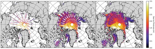
Satellite-driven SIT datasets from altimeters have larger footprints than those obtained from close-range platforms. However, due to the extremely small footprints of altimeter sensors (Figure 1), it is believed that data should be collected at intervals of at least one month in order to map the entire Arctic with a single instrument. Nevertheless, for several applications, this data collection interval is not suitable for detecting rapid changes in sea ice volume. Based on an empirical relationship between emissivity and ice thickness, SIT can also be estimated using brightness temperature (TB) data from passive microwave (PMW) sensors, such as the Advanced Microwave Scanning Radiometer 2 (AMSR2). Compared with altimeter sensors, the larger footprint of the PMW sensors enables the generation of daily thickness maps for the pan-Arctic region. Surface salinity inversely correlates with ice thickness due to the relationship between the surface brine volume fraction and the dielectric properties of sea ice at microwave frequencies (Naoki et al. 2008; Vant, Ramseier, and Makios 1978). However, microwave radiometric signals are theoretically inadequate to observe radiation emitted from the vertical features of the ice layer, which is required for SIT estimation (Lee et al. 2020; Naoki et al. 2008). The Soil Moisture and Ocean Salinity (SMOS) mission uses the 1.4 GHz (L-band) channel, characterized by significant sea ice penetration depth (Kaleschke et al. 2012). It has been used to retrieve the SIT of thin ice (up to 0.5 m) during the Arctic freezing period. However, sea ice penetration depth becomes smaller at higher frequencies in most PMW sensors. Of note, the polarization ratio (PR) of TB between horizontal and vertical polarizations has often been considered in thin ice thickness algorithms (Iwamoto et al., 2014; Martin et al. 2004; Tamura and Ohshima 2011). Yoshizawa, Shimada, and Cho (2018) used the gradient ratio (GR) of the vertical polarization of the AMSR2 18 GHz and 36 GHz channels to estimate the flat first-year ice draft (i.e. the ice thickness below the waterline). They evaluated the data using in situ ice draft from a moored IPS in the Chukchi Abyssal Plain. For these reasons, PMW-based SIT estimation studies have been limited to first-year or thin ice retrievals. As a multi-sensor data merging approach, Ricker et al. (2017) proposed an interpolation scheme using SIT data from CS2 and SMOS to generate a weekly Arctic-wide SIT product. However, this weekly product used 2–4 weekly SIT means as the background. Based on previous studies, current PMW-based SIT retrievals are limited to thin ice, and no operational daily SIT product exists for all ice types from any satellite remote sensing data. However, some weekly or monthly averaged products generated daily are available from the Alfred Wegener Institut (AWI; https://awi.de) and the National Snow & Ice Data Center (NSIDC; https://nsidc.org).

Figure 1. Examples of gridded Arctic sea ice thickness (SIT) maps derived from CryoSat-2 (CS2): 1-day (left, 1 February 2019); 14-day (middle, February 1–14); and 28-day (right, February 1–28) composites

Deep learning (DL), an emerging topic in the machine learning community, attempts to model high-level abstraction in big data (LeCun, Bengio, and Hinton 2015). Deep learning is motivated by mimicking the learning process of the human brain, which often interactively learns from past experiences. In recent studies, a variety of DL architectures, such as multi-layer perceptron (MLP) (Gardner and Dorling 1998), convolutional neural networks (CNNs) (Krizhevsky, Sutskever, and Hinton 2017), and recurrent neural networks (RNN) (Sak, Senior, and Beaufays 2014) have been proposed and applied in diverse fields of study, yielding outstanding results (Zou et al. 2015). Several studies have also been investigated using DL for retrievals of sea ice properties. Chi et al. (2019) proposed an MLP-based Arctic sea ice concentration (SIC) retrieval algorithm that used AMSR2 observations and high-resolution SIC derived from Moderate Resolution Imaging Spectroradiometer (MODIS) data as reference data. In their study, DL-based SIC values exhibited better agreements than other retrieval algorithms, especially in the 20–80% SIC zones. Wang et al. (2016) utilized CNN to estimate SIC from synthetic aperture radar (SAR) images during the melt season. This approach was robust regarding the effects of the incidence angle, noise, wind, and melt and produced high-resolution SIC estimates in regions with low ice concentrations. Chi and Kim (2017) obtained the first SIC predictions using RNN without incorporating additional ocean–atmosphere variables. Their study yielded comparable September forecasts to the results of various statistical and numerical models obtained via the Sea Ice Outlook (https://arcus.org/sipn/sea-ice-outlook).

In this study, we propose a novel SIT retrieval algorithm using a state-of-the-art CNN approach for all ice types and daily mapping from AMSR2 PMW data, which are not generally used for retrieving ice thicknesses. The retrieval model uses a CNN-based ensemble approach that concatenates multiple types of input features generated by the proposed mathematical operations to estimate SIT from the AMSR2 data. The SIT retrieval model exploits hidden and nonlinear relationships inherent in multiple AMSR2 channels, not often captured by traditional linear models. Although the reported CS2 SIT measurements have large errors and high uncertainties for observations of ice thicknesses less than 1 m, due in part to the limitation imposed by the radar’s pulse width, it is one of the most widely used SIT products (Kurtz, Galin, and Studinger 2014; Laxon et al. 2013; Tilling, Ridout, and Shepherd 2018). A goal of this study is to produce daily SIT maps over the entire Arctic from AMSR2 data at 25 km spatial resolution. Therefore, SIT data derived from CS2 that have been validated with in situ data (Laxon et al. 2013; Tilling, Ridout, and Shepherd 2018) were used as a reference to train and evaluate the model, and the estimated SIT values from AMSR2 showed good statistical agreements with CS2-based SITs. However, for thin ice measurements, which contain large errors and high uncertainties similar to CS2-based estimations, SIT retrievals from the proposed model were compared with daily SMOS-estimated SIT values. Lastly, a feature importance test using feature-denial experiments was conducted to explain which feature made the largest statistical contribution to the retrievals.

2. Datasets

2.1 AMSR2 brightness temperatures as input variables

The AMSR2 is onboard the Global Change Observation Mission-Water 1 (GCOM-W1), a sun-synchronous and near-polar orbiting platform successfully placed into orbit in May 2012. The AMSR2 records data at seven frequencies (6.9, 7.3, 10.6, 18.7, 23.8, 36.5, and 89 GHz) for horizontal (H) and vertical (V) polarization (Okuyama and Imaoka 2015). To mitigate the impacts of different antenna patterns (footprints) for the AMSR2 channels, re-sampled and gridded Level-3 TB data (25 km spatial resolution) were obtained from the Globe Portal System (https://gportal.jaxa.jp), which is operated by the Japan Aerospace Exploration Agency (JAXA). In this study, the AMSR2 Level-3 TB data were used as input variables.

2.2 Gridded CryoSat-2 sea ice thickness (SIT) as a target variable

Following the failure, CS2 was placed into a low-Earth orbit in April 2010 with an orbital inclination of 92°, enabling coverage up to 88° N. The SAR Interferometric Radar Altimeter (SIRAL) is the primary instrument aboard the CS2 that measures ice elevation using radar. It has a footprint of approximately 0.3 km × 1.5 km along-track and cross-track, respectively (Laxon et al. 2013). Once the sea ice freeboard is estimated from the CS2 radar waveforms, converting to SIT is straightforward using the hydrostatic equilibrium equation as follows (Alexandrov et al. 2010; Kurtz, Galin, and Studinger 2014; Laxon et al. 2013):

$\mathrm{S}\mathrm{I}\mathrm{T}=F\frac{{\rho }_w}{{\rho }_w-{\rho }_I}+S\frac{{\rho }_s}{{\rho }_w-{\rho }_I}$

where F is the sea ice freeboard, S is the snow depth, and ${\rho }_w,{\rho }_I,{\rho }_s$ are the densities of seawater, sea ice, and snow, respectively. Based on the assumption that ${\rho }_w,{\rho }_I,{\rho }_s$ are known parameters, the parameterization of snow depth on sea ice is the most challenging, as it is not routinely measured. Since there are many approaches to converting freeboard into thickness using different parameter assumptions (Alexandrov et al. 2010; Kwok et al. 2019; Laxon et al. 2013), we used the converted daily SIT trajectory data obtained from the AWI to minimize uncertainties in the conversion process.

The AMSR2 Level-3 TB data include multiple tracks because the ground tracks overlap at high latitudes, and the overlapping regions increase with latitude. Differences in acquisition times may be responsible for the differences between the CS2 and PMW-based SIT values due to sea ice drift from wind forcing and ice-ocean interactions (Nakayama, Ohshima, and Fukamachi 2012). However, because the daily ice drift rate in the Arctic is less than 10 km/day, which is smaller than the spatial resolution (25 km) of the AMSR2 data used in this study (Durner et al. 2017; Lund et al. 2018), time differences within a single day were not considered. Most CS2-based SIT products are often output onto a Polar Stereographic or EASE 2.0 grid due to the large variations in SIT estimates from CS2 (Laxon et al. 2013; Kurtz, Galin, and Studinger 2014; Tilling, Ridout, and Shepherd 2018). Therefore, in this study, the daily SIT trajectories from the CS2 data were mapped onto the same Polar Stereographic 25 km grid cells as those used for the AMSR2 data. Samples of gridded Arctic SIT maps derived from the CS2 data are shown in Figure 1. The weighted arithmetic mean, which is based on the individual thickness uncertainties, was used to calculate the average ice thickness within each grid cell as follows:

$\overline{\mathrm{S}\mathrm{I}\mathrm{T}}=\sum _{i=1}^N\frac{\mathrm{S}\mathrm{I}{\mathrm{T}}_i}{{\sigma }_{\mathrm{S}\mathrm{I}{\mathrm{T}}_i}^2}\cdot {\sigma }_{\overline{\mathrm{S}\mathrm{I}\mathrm{T}}}^2$

${\sigma }_{\overline{\mathrm{S}\mathrm{I}\mathrm{T}}}=\sqrt{1/\sum _{i=1}^N\frac{1}{{\sigma }_{\mathrm{S}\mathrm{I}{\mathrm{T}}_i}^2}}$

where N is the number of SIT measurements within a grid cell, ${\sigma }_{\mathrm{S}\mathrm{I}\mathrm{T}}$ is the uncertainty of the ice thickness retrieval, and ${\sigma }_{\overline{\mathrm{S}\mathrm{I}\mathrm{T}}}$ is the random uncertainty. Since the mean SIT uncertainty depends on the number of data points in a grid cell, the mean uncertainty cannot be interpolated onto a different grid. Therefore, ${\sigma }_{\overline{\mathrm{S}\mathrm{I}\mathrm{T}}}$ was calculated for each grid cell, and the SIT values with high random uncertainties (three standard deviations from the mean as a cutoff) were excluded from the SIT retrieval model (the percentage of the excluded data was approximately 3.5%). Hereafter, CS2-derived SIT values are the weighted arithmetic mean SIT corresponding to a 25 km grid cell and used as a target variable in this study.

3. Methods

Convolutional neural networks provide suitable techniques by learning contextual features and are widely used in image classification tasks (Krizhevsky, Sutskever, and Hinton 2017; Yu et al. 2017). Generally, convolutions are performed in the spatial domain but can be performed in the one-dimensional (1D) spectral domain, such as for hyperspectral or multi-variable data (Li, Zhang, and Zhang 2014; Maggiori et al. 2016). Multi-layer perceptron is a widely used type of feed-forward neural network based on back-propagation. However, MLP is unsuitable for more advanced tasks because it consists of fully connected layers in which each perceptron is connected to every other perceptron. Since the total number of learnable parameters can become extremely large, this results in redundancy when there are many dimensions. In contrast, CNN often uses fewer parameters than a fully connected network, and learns and generalizes features from the input domain.

Similar to general CNN architectures, 1D-CNN consists of two parts: 1) feature extraction and 2) regression or classification (Ince et al. 2016; Krizhevsky, Sutskever, and Hinton 2017; Peng, Liu et al., 2018a; Huang et al. 2019). Feature extraction has convolutional and pooling layers, and the regression/classification has fully-connected dense and dropout layers. The flattened layer between the first and second parts of the CNN exists to connect the two parts, with each convolutional and dense layer having an activation function. To create feature maps, the convolutional layers use a set of learnable filters connected to an input. Each filter convolves across the variables and computes the dot products. A pooling layer is inserted between successive convolutional layers, reducing the number of parameters, generalizing the feature maps, and preventing overfitting of the training data. To create final nonlinear combinations of features and make decisions, each of the fully connected layers, which are regular feed-forward neural-network layers, has full connections to all of the activations in the previous layer (LeCun, Bengio, and Hinton 2015; Krizhevsky, Sutskever, and Hinton 2017).

3.1 Feature augmentation strategy

In conventional machine learning tasks, the use of a large number of input features does not always guarantee higher accuracy, owing to the curse of dimensionality (Bellman 2015). In contrast, recent advanced DL approaches have been able to handle this limitation by combining improved optimization algorithms, big data, and advanced machines. The general form of a DL algorithm, including that of a 1D-CNN, is based on “add” operations between the input features to determine their weights or convolutional filters instead of “product” operations (Qu et al. 2018). For instance, output $\left(\mathrm{y}\right)$ of the hidden layer in DL can be calculated using $w_1{\mathrm{x}}_1+w_2{\mathrm{x}}_2+\cdots +w_n{\mathrm{x}}_n$ where $w,\mathrm{x},n$ are weights, input features, and the number of input features, respectively. Direct mathematical operations between two or more input features such as $w_1{\mathrm{x}}_1{\mathrm{x}}_2+w_2{\mathrm{x}}_1{\mathrm{x}}_3+\cdots +w_{n-1}{\mathrm{x}}_1{\mathrm{x}}_n$ will never occur.

Since we wanted to determine the theoretically unknown relationship between PMW signals and ice thickness values using DL, which has not been investigated in the current PMW-based SIT retrieval algorithms, exploiting features generated by “product” operations may be worthwhile. Therefore, we defined some inter-feature operations using the inverse, logarithm, Hadamard product, and normalized differences between TB channels (NDTB) in addition to the original 14 channels in the AMSR2 TB data, as listed in Table 1. In particular, the expression for NDTB $\left(v_{1}p,v_{2}p\right)$ was inspired by the widely used PR ($v$) and GR $\left(v_{1}p,v_{2}p\right)$ for the retrieval of sea ice properties from PMW data. The expression for PR is given by the normalized difference between the H- and V-polarized TB at a single frequency ($v$), and GR is the spectral gradient of TB between two different frequencies ($v_1,v_2$) for the polarized component ($p$) (Markus and Cavalieri 2000). Considering all of the combinations from the original 14 features, a total of 357 features were obtained for the extended model inputs instead of the original 14 AMSR2 TB features. It is uncertain whether these additional features are physically meaningful. However, finding and defining the hidden and unknown relationships between the additional features may be helpful for AMSR2-based SIT retrievals for all ice types. In particular, a few NDTBs have been used in retrieval algorithms for studies of ice concentration, type, thickness, and snow depth, as shown in Table 2. In addition, they could be used to estimate SIT directly from the PMW data without a freeboard (or draft)-thickness conversion.

Table 1. Input features for the proposed AMSR2-based sea ice thickness (SIT) retrieval model by feature augmentation

Input feature	Description	Number of features
$\mathrm{T}\mathrm{B}\left(v,p\right)$	Original $p$ polarized brightness temperature (TB) at a single frequency $\nu$	14
$1/\mathrm{T}\mathrm{B}\left(v,p\right)$	Inverse of $\mathrm{T}\mathrm{B}\left(v,p\right)$	14
$log\mathrm{T}\mathrm{B}\left(v,p\right)$	Logarithm of TB(ν,p)	14
$1/log\mathrm{T}\mathrm{B}\left(v,p\right)$	Inverse-logarithm of $\mathrm{T}\mathrm{B}\left(v,p\right)$	14
$\mathrm{T}\mathrm{B}\left(v_1,p\right)\circ \mathrm{T}\mathrm{B}\left(v_2,p\right)$	Hadamard product of two frequency channels $\left(v_1,v_2\right)$ for $p$ polarization	105
$1/\left(\mathrm{T}\mathrm{B}\left(v_1,p\right)\circ \mathrm{T}\mathrm{B}\left(v_2,p\right)\right)$	Inverse of $\mathrm{T}\mathrm{B}\left(v_1,p\right)\circ \mathrm{T}\mathrm{B}\left(v_2,p\right)$	105
$\frac{\left(\mathrm{T}\mathrm{B}\left(v_1,p\right)-\mathrm{T}\mathrm{B}\left(v_2,p\right)\right)}{\left(\mathrm{T}\mathrm{B}\left(v_1,p\right)+\mathrm{T}\mathrm{B}\left(v_2,p\right)\right)}$	Normalized difference TB (NDTB) between two different frequencies $\left(v_1,v_2\right)$ or the polarization ($p$)	91

Note: $p$ denotes horizontal or vertical polarization. $\nu$ denotes the AMSR2 channels (6.9, 7.3, 10.6, 23.8, 36.5, and 89 GHz)

Table 2. Relationship between NDTB feature and the corresponding ratio widely used in retrieval algorithms of sea ice properties

NDTB feature	Corresponding polarization ratio (PR) or gradient ratio (GR)	Applications
NDTB(18.7H, 18.7V)	PR(18.7)	∙ Ice concentration (Cavalieri, Gloersen, and Campbell 1984; Gloersen and Cavalieri 1986; Markus and Cavalieri 2000) ∙ Ice type (Aaboe et al. 2016)
NDTB(36.5H, 36.5V)	PR(36.5)	∙ Ice concentration (Comiso 1986) ∙ Thin ice thickness (Martin et al. 2004; Tamura and Ohshima 2011; Iwamoto, Ohshima, and Tamura 2014)
NDTB(89H, 89V)	PR(89)	∙ Ice concentration (Markus and Cavalieri 2000) ∙ Thin ice thickness (Tamura and Ohshima 2011; Iwamoto, Ohshima, and Tamura 2014) ∙ Ice type (Aaboe et al. 2016)
NDTB(89V, 36.5V)	GR(89V, 36.5V)	∙ Fast ice mask (Iwamoto, Ohshima, and Tamura 2014)
NDTB(36.5V, 18.7V)	GR(36.5V, 18.7V)	∙ Ice concentration (Cavalieri, Gloersen, and Campbell 1984; Gloersen and Cavalieri 1986) ∙ Snow depth (Markus and Cavalieri 1998) ∙ Flat first-year ice draft (Yoshizawa et al.) ∙ Ice type (Aaboe et al. 2016)
NDTB(89V, 18.7V)	GR(89V, 18.7V)	∙ Ice concentration (Markus and Cavalieri 2000)
NDTB(89H, 18.7H)	GR(89H, 18.7H)	∙ Ice concentration (Markus and Cavalieri 2000)

3.2 Ensemble one-dimensional convolutional neural network

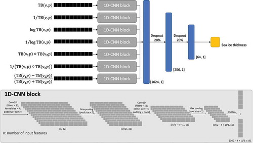
Owing to the nature of 1D-CNN, which explores neighboring features using convolutional filters, extracting meaningful information may be inefficient when the features are distant or physically uncorrelated. For example, if the number of input features is large, it is difficult to extract some information from the first and the last features unless a large kernel size or very deep network architecture is used. To overcome this limitation, this study split the input features into seven branches based on the feature augmentation rules listed in Table 1. We then developed a 1D-CNN-based ensemble model with multiple inputs and different modalities. The proposed model takes seven types of features as inputs, each having a different size. Figure 2 shows the proposed model architecture, along with the shape of each layer. Separate feature extractions of the 1D-CNN model blocks are operated on each feature type (gray blocks in Figure 2), with the results from all branches concatenated (blue blocks in Figure 2) for the final SIT retrieval (yellow block in Figure 2). The widely used rectified linear unit (ReLU) (Agarap 2018) and adaptive moment estimation (Adam) (Kingma and Ba 2014) with a 10⁻⁴ learning rate were used as the activation function for the convolutional and dense layers and as the gradient descent optimization algorithm, respectively. The mean absolute error (MAE) was used to calculate the loss due to its robustness to outliers. The dropout in the dense layers was used to learn about more robust features and prevent overfitting (Srivastava et al. 2014). Bayesian optimization was employed to optimize network configurations (hyperparameters) using small subsets of the data (Brochu, Cora, and De Freitas 2010). The Keras framework (https://keras.io) was used to build the 1D-CNN to retrieve the SIT from the AMSR2 TB data with TensorFlow (https://tensorflow.org) as a backend.

Figure 2. Network architecture of the proposed ensemble one-dimensional convolutional networks (1D-CNN) model for retrieving SIT from augmented AMSR2 brightness temperature (TB) data. Black layers denote each input feature group, as defined in Table 1, and pass through a 1D-CNN block. The results from each 1D-CNN block then concatenate and deliver to the dense layer parts (blue layers) for SIT retrieval

3.3 Model training

Due to the high uncertainties in summer SIT retrievals, we estimated the SIT for the freezing season (October to April), similar to other SIT retrieval studies/products (Iwamoto, Ohshima, and Tamura 2014; Kaleschke et al. 2012; Kurtz, Galin, and Studinger 2014; Kwok et al. 2019; Laxon et al. 2013; Lee et al. 2020; Ricker et al. 2017; Yoshizawa, Shimada, and Cho 2018; Lee et al. 2020). To develop a robust SIT retrieval model, we trained using a set of corresponding AMSR2 TB and CS2 SIT data acquired from two freezing seasons (October 2015–April 2016 and October 2016–April 2017; 662,299 samples), validated using data acquired from October 2017–April 2018 (332,049 samples), and tested using data acquired from October 2018–April 2019 (335,299 samples). Pixels near the coastlines were excluded to minimize land spillover effects that are misclassified sea ice pixels because of mixed land-ocean areas within the sensor’s field of view (Cavalieri et al. 1999). Pixels with SICs of less than 15%, a widely used threshold value to determine sea ice extent (Vinnikov et al. 1999), were also excluded as they are highly mixed pixels of ice and water signals (Chi et al. 2019). The TB data from the ascending and descending passes were averaged and used to develop the ensemble 1D-CNN model, as illustrated in Figure 2.

We performed cross-validation by shuffling the years for training/validation/test sets to avoid accidental results due to fixed datasets. For example, one randomized set used data from October 2014–April 2015 and October 2017–April 2018 for training, data from October 2016–April 2017 for validation, data from October 2012–April 2013 for testing, etc. The results confirmed that the model scores were stable in time and were insensitive to the randomness. Therefore, in this study, we conducted experiments using data from October 2015–April 2016 and October 2016–April 2017 as training sets, data from October 2017–April 2018 as validation sets, and data from October 2018–April 2019 as testing sets.

4. Results and discussion

4.1 Model comparison

We first evaluated the performance of the proposed ensemble model based on the number of input features and model architectures. Although DL approaches showed promising results in many applications, it does not always guarantee better outcomes. Therefore, we chose a random forest (RF) regression model as the baseline model because of its popularity and performance in various machine learning applications (Fernández-Delgado et al. 2014). Five experimental cases were considered: 1) RF using the original 14 features; 2) RF using the extended 357 features; 3) 1D-CNN using the original 14 features; 4) 1D-CNN using the extended 357 features; 5) the proposed ensemble 1D-CNN using the extended 357 features. For the RF models, a grid search was used to determine the best values of the hyperparameters (number of trees, maximum tree depths, and the maximum number of features). For the conventional 1D-CNN models, one of seven input CNN blocks and dense layers (gray and blue blocks, respectively, in Figure 2) were directly connected without the concatenate layer. The training process of the CNN-based models continued iterating using the entire set of training samples, which were exposed to the network until the loss function for the validation data reached a minimum. With a 16,384 training batch size, 1D-CNN (14 features) and 1D-CNN/ensemble 1D-CNN (357 features) converged to minimum loss values after approximately 100,000 and 70,000 training epochs, respectively, on an NVIDIA^TM Tesla V100 with 32 GB of memory.

Table 3 summarizes MAE, root mean square error (RMSE), bias, the Pearson correlation coefficient, and computational time according to the model architectures and the number of input features for the unseen test data (October 2018–April 2019) (Note: p-values of all models from Student’s t-tests were < 0.001). The use of extended features proposed in this study contributed to improved SIT estimations from the AMSR2 data, and the proposed ensemble model further yielded better agreements with the gridded CS2-based SIT estimates. The proposed ensemble model with the extended input features produced the most accurate outcomes. Furthermore, due to there being 10% fewer trainable parameters for the proposed ensemble model (1,557,073 versus 1,707,569), it was more computationally efficient than the conventional 1D-CNN-based models with the same number of input features. Although exploiting fewer features accelerated the model training and provided better estimations than the RF, the error of the proposed model was about half that of the 14-feature 1D-CNN model (MAE: 11.99 cm versus 25.00 cm; RMSE: 18.38 cm versus 35.33 cm).

Table 3. Statistical model comparisons (mean absolute error (MAE), root mean square error (RMSE), bias, and the Pearson correlation coefficient) with computational time using test sets according to the model architectures and number of input features

Model	Number of input features	MAE (unit: m)	RMSE (unit: m)	Bias (unit: m)	Correlation	Computational run-time
Random forest	14	0.3435	0.4601	0.1274	0.8728	~ 0.2 h (CPU)
	357	0.3216	0.4359	0.1007	0.8842	~ 0.2 h (CPU)
1D-CNN	14	0.2500	0.3533	0.0561	0.9267	~ 3 h (GPU)
	357	0.2115	0.3063	0.0767	0.9464	~ 22 h (GPU)
Ensemble 1D-CNN	357	0.1199	0.1838	0.0187	0.9800	~ 20 h (GPU)

Note: Random forest models were trained using CPU cores of Intel Xeon 6242 R (20 Cores, 3.10 GHz) with 512 GB memory. Deep learning models were trained using GPU cores of NVIDIA Tesla V100 (5,120 CUDA cores, 640 Tensor cores, 32 GB memory).

4.2 Quantitative accuracy assessment using gridded CryoSat-2 estimates

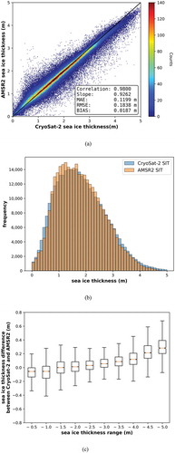
First, statistical comparisons were conducted between the AMSR2-derived daily SIT values estimated by the ensemble 1D-CNN (SIT_AMSR2) and the corresponding SIT values derived from the gridded CS2 data (SIT_CS2). The SIT_CS2 was evaluated using fine-scale in situ measurements acquired from OIB, IPS, or ULS (Laxon et al. 2013; Tilling, Ridout, and Shepherd 2018). Figure 3(a) shows the SIT_AMSR2 versus SIT_CS2 for the unseen test data (October 2018–April 2019), with the number of pixels denoted by the color intensity. In statistical terms, 11.99 cm of MAE, 18.38 cm of RMSE, and a near-zero bias for the test data were achieved. Remarkable correlations between the SIT_AMSR2 and SIT_CS2 were observed in the scatter plot. The Pearson correlation coefficient was 0.98, and the regression slope was near unity (0.93). The distribution of most sample points in the scatter plot was very close to the 1:1 line. Figure 3(b) illustrates a histogram of SIT_AMSR2 (orange) and SIT_CS2 (blue), with a 10 cm bin width. While the AMSR2-based SIT retrieval model showed a relative weakness in estimating SITs of less than 1.3 m, it exhibited a better estimation capacity for ice with thicknesses of 1.3–4 m. Figure 3(c) is a boxplot of the differences in SIT between AMSR2 and CS2 (SIT_CS2 – SIT_AMSR2) according to SIT ranges. The median thickness differences (orange lines) tended to increase slightly from the negative to positive values as the sea ice thickened yet generally formed around zero, and the whiskers were approximately equal on both sides of the box for thicknesses up to 4 m. In particular, SITs between 1.5 and 3 m exhibited better agreements than the other ranges due to the higher number of training samples in this range.

Figure 3. Statistical accuracies of the proposed SIT retrieval model using the test set: (a) Scatter plot of gridded CS2-estimated SIT (SIT_CS2; x-axis) vs. AMSR2-estimated SIT (SIT_AMSR2; y-axis) values; (b) histogram of SIT_CS2 (blue) and SIT_AMSR2 (orange) with a 10 cm bin size; (c) boxplot of SIT differences between CS2 and AMSR2 according to ice thickness ranges

Overall, errors can be attributed to two sources. First, the differences in spatial resolution and acquisition times between the AMSR2 and CS2 may have resulted in a few misestimated samples. Although our labeled matched samples used for model training and testing were selected carefully based on pre-defined criteria (Section 2.2), multiple thickness measurements from CS2 corresponding to one 25 km AMSR2 grid cell may have caused errors. Second, AMSR2 tended to underestimate SIT as the sea ice thickened, as seen in Figure 3. The number of samples in the thick ice range (> 4 m) was much smaller than in the 1–3 m range. These imbalanced samples in thick SIT ranges can cause underestimations in the thick ice estimates.

We generated daily SIT_AMSR2 maps from October 2012–April 2020 and evaluated them by making seasonal and monthly statistical accuracy (MAE, RMSE, and correlation) comparisons with corresponding gridded SIT_CS2 values as listed in Table 4. All of the p-values from Student’s t-tests for the daily data were less than 0.05, implying a statistically significant difference between the two datasets at a confidence level of 95%. Since the developed ensemble 1D-CNN model was exposed to data from October 2015–April 2018 for model training and validation, the seasonal statistics for these periods were better than those for data not exposed to the model (October 2013–April 2015; October 2018–April 2020). Overall, the seasonal averages for the unseen periods were consistent throughout the unseen periods and were not significantly different from those for the test period (MAE: 13.28 cm versus 13.43 cm; RMSE: 18.07 cm versus 18.23 cm; Correlation: 0.9800 versus 0.9816). In monthly comparisons, SIT_AMSR2 estimates in October and April exhibited weak agreements with SIT_CS2 compared to those from November–March and the seasonal means. One possible explanation for this is that October and April are the freezing and melting onsets of Arctic sea ice, respectively (Markus, Stroeve, and Miller 2009; Peng, Steele et al., 2018b). Therefore, more variations in sea ice dynamics within a 25 km grid can exist during these periods. While the accuracy from November–March was relatively stable, accuracy tended to decrease slightly as sea ice extents increased because of the increased number of sea ice pixels to be calculated in the statistical comparisons (Comiso et al. 2008). These results indicate that the retrieval model developed herein is statistically robust regarding unseen data and generalized since the proposed DL model was trained using sufficient training and validation samples from three Arctic winter seasons. Therefore, the proposed model is expected to be suitable for future operational generation of daily AMSR2-based SIT products.

Table 4. Comparisons of seasonal and monthly MAE, RMSE, and the Pearson correlation coefficient between the daily AMSR2 and CryoSat-2-derived sea ice thickness

MAE (unit: m)	Seasonal average	Oct	Nov	Dec	Jan	Feb	Mar	Apr
2012–2013*	0.1219	0.1387	0.1138	0.1157	0.1124	0.1094	0.1227	0.1407
2013–2014*	0.1334	0.1282	0.1174	0.1176	0.1244	0.1347	0.1403	0.1710
2014–2015*	0.1405	0.1569	0.1247	0.1275	0.1238	0.1296	0.1410	0.1804
2015–2016^1	0.0370	0.0474	0.0268	0.0234	0.0363	0.0283	0.0368	0.0599
2016–2017^1	0.0335	0.0462	0.0293	0.0250	0.0249	0.0221	0.0286	0.0587
2017–2018^2	0.0513	0.0604	0.0433	0.0390	0.0425	0.0565	0.0509	0.0668
2018–2019^3*	0.1343	0.1586	0.1202	0.1221	0.1178	0.1240	0.1313	0.1659
2019–2020*	0.1340	0.1447	0.1265	0.1225	0.1279	0.1289	0.1321	0.1551
Unseen average	0.1328	0.1454	0.1205	0.1211	0.1213	0.1253	0.1335	0.1626
RMSE (unit: m)	Seasonal average	Oct	Nov	Dec	Jan	Feb	Mar	Apr
2012–2013*	0.1658	0.1834	0.1566	0.1586	0.1553	0.1516	0.1676	0.1876
2013–2014*	0.1810	0.1684	0.1582	0.1635	0.1735	0.1838	0.1909	0.2286
2014–2015*	0.1927	0.2064	0.1716	0.1776	0.1721	0.1819	0.1957	0.2440
2015–2016^1	0.0859	0.0915	0.0717	0.0685	0.0848	0.0773	0.0925	0.1148
2016–2017^1	0.0828	0.0917	0.0787	0.0747	0.0758	0.0731	0.0788	0.1072
2017–2018^2	0.1066	0.1143	0.0974	0.0923	0.0935	0.1178	0.1068	0.1240
2018–2019^3*	0.1823	0.2060	0.1658	0.1709	0.1614	0.1742	0.1802	0.2173
2019–2020*	0.1818	0.1892	0.1726	0.1685	0.1747	0.1794	0.1827	0.2053
Unseen average	0.1807	0.1907	0.1650	0.1678	0.1674	0.1742	0.1834	0.2165
Correlation	Seasonal average	Oct	Nov	Dec	Jan	Feb	Mar	Apr
2012–2013*	0.9764	0.9697	0.9783	0.9764	0.9813	0.9811	0.9759	0.9718
2013–2014*	0.9838	0.9836	0.9867	0.9866	0.9824	0.9829	0.9841	0.9807
2014–2015*	0.9798	0.9714	0.9845	0.9841	0.9837	0.9804	0.9785	0.9763
2015–2016^1	0.9922	0.9784	0.9949	0.9967	0.9895	0.9969	0.9963	0.9929
2016–2017^1	0.9938	0.9899	0.9971	0.9975	0.9948	0.9936	0.9921	0.9914
2017–2018^2	0.9891	0.9849	0.9942	0.9938	0.9940	0.9866	0.9838	0.9868
2018–2019^3*	0.9816	0.9729	0.9892	0.9861	0.9845	0.9795	0.9805	0.9786
2019–2020*	0.9784	0.9711	0.9821	0.9827	0.9794	0.9790	0.9774	0.9771
Unseen average	0.9800	0.9737	0.9842	0.9832	0.9823	0.9806	0.9793	0.9769

¹Training data; ²Validation data; ³Test data; *Unseen data

4.3 Quantitative accuracy assessment using gridded operational IceBridge measurements

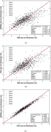
We evaluated the SIT_AMSR2 estimated using the proposed method with in situ SITs collected from OIB missions (SIT_OIB) from 2012 to 2019. However, there were significant differences in the spatiotemporal scales between the 25 km resolution AMSR2 grid and the fine-scale in situ data. Similar to SIT_CS2, multiple OIB measurements were associated with the same SIT_AMSR2 value. For this reason, the OIB data were gridded on the same 25 km grid using the same approach used in the CS2 to AMSR2 grid conversions (see Section 2.2). We selected 740 spatiotemporally matched samples from gridded AMSR2, CS2, and OIB datasets for pixel-to-pixel cross-comparisons. Figure 4 illustrates this cross-comparison, whose statistics were calculated using the same metrics as the previous comparisons. As shown in Figure 4(a), 47 cm of MAE and 68 cm of RMSE, with a correlation of 0.76, were obtained between SIT_AMSR2 and gridded SIT_OIB, which are much larger than the error between SIT_AMSR2 and SIT_CS2 (see Figure 3(a)). Two possible reasons may explain these differences. First, the spatiotemporal resolutions of the two data sources significantly differed. Although we assumed the gridded SIT_CS2 as a reference and used them to compare with SIT_AMSR2 in the previous experiments (Section 4.2), the SIT_OIB data were acquired from completely different instruments. Second, CS2-derived SIT estimates used climatological snow depth values and were multiplied over first-year ice using a factor of 0.5 due to a significantly higher fraction of first-year ice (Kurtz and Farrell 2011; Hendricks, Ricker, and Helm 2016). However, snow depths during the IceBridge campaigns were derived from the snow radar (Kurtz and Farrell 2011). Additionally, different ice density assumptions in freeboard to thickness conversions may have resulted in large differences between the datasets (Kurtz, Galin, and Studinger 2014). While the CS2 SIT product used values of 916.7 kg/m³ and 882 kg/m³ for first-year and multi-year ice, respectively (Laxon et al. 2013; Hendricks, Ricker, and Helm 2016), the OIB SIT used 915 kg/m³ (Kurtz and Farrell 2011; Kurtz et al. 2013). However, as shown in Figure 4(b), a comparison of SIT_CS2 and SIT_OIB also had a similar error level. A direct comparison of SIT_AMSR2 and SIT_CS2 for the matched samples in Figure 4(c) still had a good agreement, although the number of samples was substantially smaller than those used in Figure 3(a) (335,299 versus 740 samples). In previous studies, Laxon et al. (2013) and Tilling, Ridout, and Shepherd (2018) showed similar difference patterns between gridded SIT_CS2 and SIT_OIB measurements, although they used different samples and grid mapping scale (0.4° latitudinal by 4° longitudinal grid).

Figure 4. Statistical accuracy comparisons using 740 matched samples from gridded Operational IceBridge (SIT_OIB), SIT_AMSR2, and SIT_CS2 data: (a) Scatter plot of SIT_OIB (x-axis) vs. SIT_AMSR2 (y-axis); (b) scatter plot of SIT_OIB (x-axis) vs. SIT_CS2 (y-axis); (c) scatter plot of SIT_CS2 (x-axis) vs. SIT_AMSR2 (y-axis)

4.4 Visual inspections of AMSR2-based SIT maps

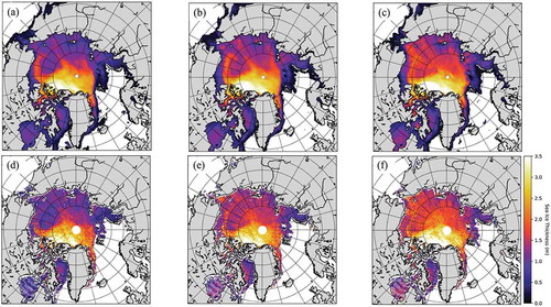
Figure 5 illustrates the AMSR2-based SIT maps over the entire Arctic Ocean for mid-October 2018 to April 2019 generated using the proposed DL method. Note that pixels with SICs of less than 15%. Due to a lack of daily SIT_CS2 data for the entire Arctic Ocean and PMW-based SIT for all ice types, direct daily visual comparisons for all AMSR2 pixels cannot be made. However, the spatial distributions of the SIT values and time-series are reasonable compared to the stage of sea ice development (Comiso et al. 2008), daily generated weekly/monthly averaged products (Ricker et al. 2017; Lee et al. 2020; Xiao et al. 2020; Artic SIT maps of Centre for Polar Observation and Modelling Data Portal (http://cpom.ucl.ac.uk)), and SIT values of adjacent pixels. Figure 6(a–c) show the monthly means of daily SIT generated from AMSR2 data, and Figure 6(d–f) show the monthly means of daily CS2 trajectories on corresponding AMSR2 grid cells for January, February, and March 2019. Overall, the distribution of the SIT_AMSR2 exhibited a fair agreement with the SIT_CS2. However, relatively high regional variations were observed in the SIT_CS2 maps, particularly in first-year ice regions. Differing spatial coverages between the two sensors may explain these variations. While the AMSR2 data yields spatially uniform measurements over the entire Arctic every day, daily CS2 measurements are sparse, especially further from the pole (i.e. first-year ice zone). This indicates that the monthly mean in a specific area contains the estimates from different days.

Figure 5. Daily generated AMSR2-derived SIT maps at 25 km spatial resolution for mid-October 2018 to April 2019

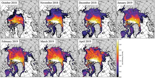
Figure 6. Monthly averaged SIT maps at 25 km spatial resolution (top row: AMSR2-derived; bottom row: CS2-derived) for January (a, d), February (b, e), and March (c, f) 2019

4.5. Comparison with the daily SMOS SIT product for thin ice

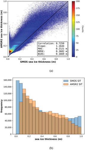
SMOS-derived SIT (SIT_SMOS) is one of the most representative daily SIT products. However, it is limited to thin ice with depths of up to approximately 0.5–1 m and depends on the ice temperature and salinity (Kaleschke et al. 2012). Kaleschke et al. (2015) and Ricker et al. (2017) found that the SIT_CS2 over thin ice (< 1 m) and in the marginal ice zone have large relative uncertainties. In this study, the SIT_AMSR2 and SIT_SMOS for corresponding thin ice pixels (< 1 m) were quantitatively and qualitatively compared. Figure 7(a) shows a plot of the SIT_AMSR2 and SIT_SMOS values with statistical comparisons for the test period (Note: p-value from Student’s t-test was < 0.001). Unlike the statistical comparison with SIT_CS2 for all ice types in the previous section (Figure 3(a)), the MAE and RMSE were calculated as approximately 21 cm and 37 cm, respectively. The estimated SIT_AMSR2 overestimated SIT compared to the SIT_SMOS (17 cm positive bias), and most of the data points in the scatter plot are above the 1:1 line. Notably, significant misestimations in sea ice pixels less than 10 cm were observed. As shown in Figure 7(b), the distribution of SIT_AMSR2 (orange) is significantly different from that of SIT_SMOS (blue). Particularly, retrievals of SIT values less than 5 cm were failed.

Figure 7. Statistical accuracy comparisons of SIT_AMSR2 and SMOS-derived SIT (SIT_SMOS) values for thin ice (< 1 m): (a) Scatter plot of SIT_SMOS (x-axis) vs. SIT_AMSR2 (y-axis) values; (b) histogram of SIT_SMOS (blue) and SIT_AMSR2 (orange) with a 5 cm bin size

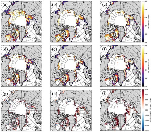
Figure 8 illustrates the SIT_AMSR2, SIT_SMOS, and their difference maps for thin ice (< 1 m) in the middle of January, February, and March 2019. The color scale in the Figure 8(g), (h), (i) is labeled SIT_AMSR2 – SIT_SMOS, with positive (SIT_AMSR2 > SIT_SMOS) and negative (SIT_AMSR2 < SIT_SMOS) differences colored red and blue, respectively. Overall, as in the scatter plot comparison, AMSR2 overestimated SIT with respect to SMOS, particularly near the coastlines of the United States, Canada, Russia, and Greenland, where first-year ice is dominant. In January images, large distributions of underestimated pixels were observed in the Beaufort, Chukchi, East Siberian, and Laptev Seas (Figure 8(a)), where SMOS masks sea ice pixels thicker than 1 m (Figure 8(d)). The Bering Strait and a small area of the Chukchi Sea were underestimated (Figure 8(g)). Overall, misestimations increased as sea ice developed. In the March images (Figure 8(c, f, i)), the AMSR2 significantly overestimated thin ice in the Baffin Bay, the western Greenland Sea, and the Barents Sea.

Figure 8. Sea ice thickness maps at 25 km spatial resolution for thin ice (< 1 m) generated from AMSR2 (top row) and SMOS (middle row), and the difference between AMSR2 and SMOS (bottom row) on January 15 (a, d, g), February 15 (b, e, h), and 15 March 2019 (c, f, i)

As addressed in previous studies that exhibited large errors over thin ice regions of CS2 (Kaleschke et al. 2015; Ricker et al. 2017), we also observed large overestimations in the SIT_AMSR2 results compared to SIT_SMOS, as shown by both statistical (Figure 7) and visual (Figure 8) analyses. The proposed retrieval model highly relies on gridded SIT_CS2 measurements with centimeter-scale differences (as shown in Section 4.2) since it assumes that gridded SIT_CS2 is a reference and even mimics the potential errors/uncertainties in the SIT_CS2 estimations over thin ice. Sparse CS2 SIT measurements in first-year ice regions and exclusion of water-contaminated pixels (SIC < 15%) resulted in insufficient samples from new or young ice for DL model training. This can be another potential reason for weak agreements with sea ice less than 10 cm.

4.6 Statistical feature importance test

Conventional SIT retrieval algorithms generally exploited the physical characteristics of ice using specific PMW channels or altimeter waveforms. However, the DL-based retrieval model developed in this study exploits all frequency/polarization channels of the AMSR2 data. Due to the unique characteristics of neural networks, which solve problems by exploiting hidden relationships inherent in multiple input features, it is difficult to physically quantify the importance of the input variables. Alternatively, we performed a feature permutation test to statistically explain which feature makes the largest contribution to the SIT retrievals. A single feature was randomly varied, while all other features were kept constant, and this process was iterated by changing the input feature. The feature significance assessment shows how the model performance decreased due to random shuffling. In this case, performance was measured using the MAE, which was used as the loss metric in model training.

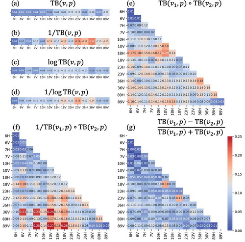
Figure 9 shows heat maps of the increased MAE values resulting from the input feature permutation tests, calculated after ten replicates. Inputs with greater increased MAE values due to random permutations were more significant for determining the SIT. Using this metric, the original TB features were not statistically significant, whereas the additional features generated by our feature augmentation strategy demonstrated greater responses. Although the logarithm TB features (Figure 9(c)) seem to be more important than the original TB features (Figure 9(a)), they were not significant. The Hadamard product of two AMSR2 channels (Figure 9(e)) had a greater effect on retrievals than that of a single feature operation (Figure 9(a–d)). Overall, the Hadamard products combining low- and high-frequency channels contributed the most to the AMSR2-based SIT retrievals. The features defined by inverse operations of the original, logarithm, and Hadamard product (Figure 9(b, d, f)) generally exhibited greater feature importance than the non-inverted features (Figure 9(a, c, e)). In particular, the five most important features were 1/(TB(89V)$\circ$TB(18V)), 1/(TB(89V)$\circ$TB(10V)), 1/(TB(89V)$\circ$TB(7V)), 1/(TB(36V)$\circ$TB(10V)), and 1/(TB(36V)$\circ$TB(7V)), which are combinations of inverse and product operations of two features. As some of the NDTB features are conventionally used to retrieve sea ice/snow properties listed in Table 2, we expected that the NDTB features would be significant. However, except for NDTB (18V, 10V) and NDTB (23V, 18V), the NDTB features were generally less critical than expected, as shown in Figure 9(g); this could be because information regarding the NDTB features may be mutually contained in the other features in the hidden layers of the neural network.

Figure 9. Increasing MAE in the AMSR2 SIT retrievals obtained from feature permutation importance tests. (a) Original $p$ polarized TB at a single AMSR2 frequency ($\nu$). (b) Inverse of $\mathrm{T}\mathrm{B}\left(\nu ,p\right)$. (c) Logarithm of $\mathrm{T}\mathrm{B}\left(\nu ,p\right)$. (d) Inverse-logarithm of $\mathrm{T}\mathrm{B}\left(\nu ,p\right)$. (e) Hadamard product of two frequency channels (v₁,v₂) for $p$ polarization. (f) Inverse of $\mathrm{T}\mathrm{B}\left({\nu }_1,p\right)\circ \mathrm{T}\mathrm{B}\left({\nu }_2,p\right)$. (g) Normalized difference TB between two different frequencies (${\nu }_1$, ${\nu }_2$) for the polarization ($p$). Note: $p$ denotes horizontal or vertical polarization. $\nu$ denotes the AMSR2 channels (6.9, 7.3, 10.6, 23.8, 36.5, and 89 GHz)

Although this statistical feature importance test may not provide a physical meaning for the relationship between the PMW signals and SIT, we derived a partial relationship between the feature importance of the proposed model and the current PMW-based SIT retrieval algorithms. Table 5 summarizes the average feature importance (according to frequency) of the features associated with a specific frequency channel from Figure 9. Features associated with frequencies higher than 10.6 GHz tended to exhibit greater significances than those associated with low-frequency channels. In particular, two of the most critical frequencies (18.7 and 36.5 GHz) are widely used in thin ice thickness retrieval algorithms (Iwamoto, Ohshima, and Tamura 2014; Yoshizawa, Shimada, and Cho 2018). The 89 GHz channel helps exclude weather-related contamination (Iwamoto, Ohshima, and Tamura 2014; Yoshizawa, Shimada, and Cho 2018). Moreover, Lee, Sohn, and Shi (2018) reported that the estimation of optical thickness associated with the scattering of ice freeboard and snow layers is possible using microwave frequencies between 10.65 and 36.5 GHz. In Lee et al. (2020), Arctic basin-scale SIT estimates from AMSR2 were demonstrated using a piecewise linear regression of optical thickness at 36.5 GHz of AMSR2 and CS2-driven ice freeboard. These studies presented new possibilities for PMW-based SIT mapping based on the assumption that the scattering optical thickness of the surface ice layer at microwave frequencies was linearly proportional to the physical thickness of the ice freeboard layer. Unfortunately, it is still difficult to clearly explain which input feature has the most physically significant effect on the retrievals. However, based on the results from the feature importance test in this study and the studies mentioned above, a partial relationship between PMW signals and SIT was explained.

Table 5. Average feature importance (according to frequency) for the features associated with a specific frequency channel. The more important frequencies have higher increased MAE values (unit: m)

	Associated frequency channel
	6.9 GHz	7.3 GHz	10.6 GHz	18.7 GHz	23.8 GHz	36.5 GHz	89 GHz
Average increased MAE	0.0819	0.0890	0.1031	0.1110	0.1048	0.1103	0.1027

Determining the significances of the input features will allow for a statistical explanation and will foreseeably help to optimize the input features of the SIT retrieval model for future operational systems. Moreover, the results demonstrate that the use of feature augmentation based on mathematical operations that cannot be exhibited in “add” operation-based general neural network architectures is more effective than only exploiting the original TB data. The absence of negative features in Figure 9 indicates that each PMW channel plays specific roles in improving the SIT retrieval model in DL hidden networks.

5. Conclusions

This study devised an ensemble 1D-CNN model and employed PMW data from the winter season to estimate daily SITs for the entire Arctic at 25 km spatial resolution, which could not be retrieved by CS2 due to ground track constraints. In general, the proposed method successfully estimated the SIT compared to the gridded SIT_CS2 and produced spatially/temporally consistent outputs in conjunction with a robust retrieval model and well-calibrated AMSR2 TB data. The following conclusions can be derived from this study.

First, most SIT retrieval studies using PMW data have been conducted to estimate thin ice thicknesses. Considering the constellation of multiple altimetry data such as Jason-3, Sentinel-3A/B, or SARAL/AltiKa may provide a better temporal resolution. However, a single altimeter sensor has been unable to map the entire Arctic Ocean on a daily scale due to small sensor footprints, and the temporal resolution of the SIT generated by merging multi-sensor data is seven days. These limitations motivated this study to use the DL approach to exploit hidden information across multiple PMW channels; thus, a DL-based retrieval model for all ice types was developed based on PMW data. Employing additional features and an ensemble approach improved the results. Second, we achieved overall MAE and RMSE accuracies of approximately 12 cm and 18 cm for unseen data, respectively, and remarkable correlations between the SIT_AMSR2 and gridded SIT_CS2. Due to the nature of machine learning, it is difficult to physically explain which AMSR2 channel made the largest contribution to the SIT estimations. Using a statistical approach, we evaluated the relative importance of the AMSR2 channels. In particular, since our approach exploited all of the AMSR2 channels, it enabled direct SIT retrievals without separate freeboard and snow depth calculations, which are hidden in the model training. Additionally, features associated with the 10.65–36.5 GHz channels exhibited more significant contributions to the AMSR2-based SIT retrievals. These frequency channels have also been incorporated into the development of a relationship between optical thickness and ice freeboard by Lee, Sohn, and Shi (2018) and Lee et al. (2020). These studies support a physical relationship between PMW signals and ice thickness for all ice types. Lastly, since the proposed retrieval model consistently generated eight-year historical data with consistent accuracy, it can be considered as a new operational SIT retrieval system for providing daily Arctic SIT data.

Although the proposed ensemble 1D-CNN model successfully estimated SITs from AMSR2 PMW data at 25 km spatial resolution and showed good agreements with gridded CS2 estimates, the uncertainties and errors in the CS2 measurements, particularly for ice less than 1 m thick, were also observed in comparisons with daily SMOS ice thickness data (Figures 7 and 8). Since the SIT retrieval model used in this study was trained using gridded SIT_CS2 as a reference for all ice thickness ranges, it may also capture uncertainties and errors in the reference data due to the characteristics of the DL models. Although 12 cm of MAE may not be trivial for new or young ice, it is worth noting that providing daily SIT maps for the entire Arctic would improve various cryosphere studies/models and support industrial applications. In addition, combining the proposed model with L-band (1.4 GHz) data from SMOS, widely used to derive thin ice thicknesses, would be worthwhile for extending this research.

Acknowledgements

Daily Level-3 gridded TB data of AMSR2, SIT trajectory data of CS2, and NASA’s OIB data are publicly available at the Globe Portal System (https://gportal.jaxa.jp) operated by JAXA, AWI (https://awi.de), and NSDIC (https://nsidc.org), respectively.

Disclosure statement

No potential conflict of interest was reported by the author(s).

Additional information

Funding

This work was supported by the Korea Polar Research Institute [PE21040].

References

- Aaboe, S., L. A. Breivik, A. Sørensen, S. Eastwood, and T. Lavergne. 2016. “Global Sea Ice Edge and Type Product User’s Manual.” OSI-403-c & EUMETSAT 250: 1–34.
- Agarap, A. F. 2018. “Deep Learning Using Rectified Linear Units (Relu).” arXiv Preprint arXiv:1803.08375.
- Alexandrov, V., S. Sandven, J. Wahlin, and O. M. Johannessen. 2010. “The Relation between Sea Ice Thickness and Freeboard in the Arctic.” Cryosphere 4 (3): 373–380. doi:https://doi.org/10.5194/tc-4-373-2010.
- Bellman, R. E. 2015. Adaptive Control Processes: A Guided Tour. Princeton, New Jersey: Princeton university press.
- Brochu, E., V. M. Cora, and N. De Freitas. 2010. “A Tutorial on Bayesian Optimization of Expensive Cost Functions, with Application to Active User Modeling and Hierarchical Reinforcement Learning.” arXiv Preprint arXiv:1012.2599.
- Cavalieri, D. J., C. L. Parkinson, P. Gloersen, J. C. Comiso, and H. H. Zwally. 1999. “Deriving Long‐term Time Series of Sea Ice Cover from Satellite Passive‐microwave Multisensor Data Sets.” Journal of Geophysical Research: Oceans 104 (C7): 15803–15814. doi:https://doi.org/10.1029/1999JC900081.
- Cavalieri, D. J., P. Gloersen, and W. J. Campbell. 1984. “Determination of Sea Ice Parameters with the Nimbus 7 SMMR.” Journal of Geophysical Research: Atmospheres 89 (D4): 5355–5369. doi:https://doi.org/10.1029/JD089iD04p05355.
- Chi, J., and H.-C. Kim. 2017. “Prediction of Arctic Sea Ice Concentration Using a Fully Data Driven Deep Neural Network.” Remote Sensing 9 (12): 1305. doi:https://doi.org/10.3390/rs9121305.
- Chi, J., H.-C. Kim, S. Lee, and M. M. Crawford. 2019. “Deep Learning Based Retrieval Algorithm for Arctic Sea Ice Concentration from AMSR2 Passive Microwave and MODIS Optical Data.” Remote Sensing of Environment 231: 111204. doi:https://doi.org/10.1016/j.rse.2019.05.023.
- Comiso, J. C. 1986. “Characteristics of Arctic Winter Sea Ice from Satellite Multispectral Microwave Observations.” Journal of Geophysical Research: Oceans 91 (C1): 975–994. doi:https://doi.org/10.1029/JC091iC01p00975.
- Comiso, J. C., C. L. Parkinson, R. Gersten, and L. Stock. 2008. “Accelerated Decline in the Arctic Sea Ice Cover.” Geophysical Research Letters 35 (1). doi:https://doi.org/10.1029/2007GL031972.
- Durner, G. M., D. C. Douglas, S. E. Albeke, J. P. Whiteman, S. C. Amstrup, E. Richardson, M. Ben‐David, and M. Ben‐David. 2017. “Increased Arctic Sea Ice Drift Alters Adult Female Polar Bear Movements and Energetics.” Global Change Biology 23 (9): 3460–3473. doi:https://doi.org/10.1111/gcb.13746.
- Fernández-Delgado, M., E. Cernadas, S. Barro, and D. Amorim. 2014. “Do We Need Hundreds of Classifiers to Solve Real World Classification Problems?” Journal of Machine Learning Research 15: 3133–3181.
- Gardner, M. W., and S. R. Dorling. 1998. “Artificial Neural Networks (The Multilayer Perceptron)—a Review of Applications in the Atmospheric Sciences.” Atmospheric Environment 32 (14–15): 2627–2636. doi:https://doi.org/10.1016/S1352-2310(97)00447-0.
- Gloersen, P., and D. J. Cavalieri. 1986. “Reduction of Weather Effects in the Calculation of Sea Ice Concentration from Microwave Radiances.” Journal of Geophysical Research: Oceans 91 (C3): 3913–3919. doi:https://doi.org/10.1029/JC091iC03p03913.
- Han, Hz., J.-I. Kim, C.-U. Hyun, S. H. Kim, J.-W. Park, Y.-J. Kwon, S. Lee, S. Lee and H.-C. Kim. 2020. “Surface roughness signatures of summer arctic snow-covered sea ice in X-band dual-polarimetric SAR.” GIScience & Remote Sensing 57(5): 650–669. doi:https://doi.org/10.1080/15481603.2020.1767857
- Hendricks, S., R. Ricker, and V. Helm. 2016. “AWI CryoSat-2 sea ice thickness data product (V1.2).” https://epic.awi.de/id/eprint/41242
- Huang, S., J. Tang, J. Dai, and Y. Wang. 2019. “Signal Status Recognition Based on 1DCNN and Its Feature Extraction Mechanism Analysis.” Sensors 19 (9): 2018. doi:https://doi.org/10.3390/s19092018.
- Hyangsun, Han, Jae-In Kim, Chang-Uk Hyun, Seung Hee Kim, Jeong-Won Park, Young-Joo Kwon, Sungjae Lee, Sanggyun Lee & Hyun-Cheol Kim. 2020. Surface roughness signatures of summer arctic snow-covered sea ice in X-band dual-polarimetric SAR, GIScience & Remote Sensing. 57: 5. 650-669, doi:https://doi.org/10.1080/15481603.2020.1767857.
- Ince, T., S. Kiranyaz, L. Eren, M. Askar, and M. Gabbouj. 2016. “Real-time Motor Fault Detection by 1-D Convolutional Neural Networks.” IEEE Transactions on Industrial Electronics 63 (11): 7067–7075. doi:https://doi.org/10.1109/TIE.2016.2582729.
- Ivanova, N., L. T. Pedersen, R. T. Tonboe, S. Kern, G. Heygster, T. Lavergne, and M. Shokr. 2015. “Inter-comparison and Evaluation of Sea Ice Algorithms: Towards Further Identification of Challenges and Optimal Approach Using Passive Microwave Observations.” The Cryosphere 9 (5): 1797–1817. doi:https://doi.org/10.5194/tc-9-1797-2015.
- Iwamoto, K., K. I. Ohshima, and T. Tamura. 2014. “Improved Mapping of Sea Ice Production in the Arctic Ocean Using AMSR-E Thin Ice Thickness Algorithm.” Journal of Geophysical Research-Oceans 119 (6): 3574–3594. doi:https://doi.org/10.1002/2013JC009749.
- Kaleschke, L., X. Tian-Kunze, N. Maas, R. Ricker, S. Hendricks, and M. Drusch. 2015. “Improved Retrieval of Sea Ice Thickness from SMOS and CryoSat-2.” Proceeding of IEEE International Geoscience and Remote Sensing Symposium (IGARSS), Milan, Italy, 5232–5235. doi: https://doi.org/10.1109/IGARSS.2015.7327014.
- Kaleschke, L., X. Tian-Kunze, N. Maass, M. Makynen, and M. Drusch. 2012. “Sea Ice Thickness Retrieval from SMOS Brightness Temperatures during the Arctic Freeze-up Period.” Geophysical Research Letters 39 (1): 39. doi:https://doi.org/10.1029/2012GL050916.
- Kingma, D. P., and J. Ba. 2014. “Adam: A Method for Stochastic Optimization.” arXiv Preprint arXiv:1412.6980.
- Koenig, L., S. Martin, M. Studinger, and J. Sonntag. 2010. “Polar Airborne Observations Fill Gap in Satellite Data.” Eos, Transactions American Geophysical Union 91 (38): 333–334. doi:https://doi.org/10.1029/2010EO380002.
- Krizhevsky, A., I. Sutskever, and G. E. Hinton. 2017. “ImageNet Classification with Deep Convolutional Neural Networks.” Communications of the Acm 60 (6): 84–90. doi:https://doi.org/10.1145/3065386.
- Kurtz, N., N. Galin, and M. Studinger. 2014. “An Improved CryoSat-2 Sea Ice Freeboard Retrieval Algorithm through the Use of Waveform Fitting.” The Cryosphere 8 (4): 1217–1237. doi:https://doi.org/10.5194/tc-8-1217-2014.
- Kurtz, N. T., and S. L. Farrell. 2011. “Large-scale Surveys of Snow Depth on Arctic Sea Ice from Operation IceBridge.” Geophysical Research Letters 38 (20): 1–5. doi:https://doi.org/10.1029/2011GL049216.
- Kurtz, N. T., S. L. Farrell, M. Studinger, N. Galin, J. P. Harbeck, R. Lindsay, V. D. Onana, B. Panzer, and J. G. Sonntag. 2013. “Sea Ice Thickness, Freeboard, and Snow Depth Products from Operation IceBridge Airborne Data.” The Cryosphere 7 (4): 1035–1056. doi:https://doi.org/10.5194/tc-7-1035-2013.
- Kwok, R., B. Panzer, C. Leuschen, S. Pang, T. Markus, B. Holt, and S. Gogineni. 2011. “Airborne Surveys of Snow Depth over Arctic Sea Ice.” Journal of Geophysical Research-Oceans 116. doi:https://doi.org/10.1029/2011JC007371.
- Kwok, R., T. Markus, N. Kurtz, A. Petty, T. Neumann, S. Farrell, and J. Wimert. 2019. “Surface Height and Sea Ice Freeboard of the Arctic Ocean from ICESat‐2: Characteristics and Early Results.” Journal of Geophysical Research: Oceans 124 (10): 6942–6959. doi:https://doi.org/10.1029/2019JC015486.
- Laxon, S. W., K. A. Giles, A. L. Ridout, D. J. Wingham, R. Willatt, R. Cullen, and M. Davidson. 2013. “CryoSat-2 Estimates of Arctic Sea Ice Thickness and Volume.” Geophysical Research Letters 40 (4): 732–737. doi:https://doi.org/10.1002/grl.50193.
- LeCun, Y., Y. Bengio, and G. Hinton. 2015. “Deep Learning.” Nature 521 (7553): 436–444. doi:https://doi.org/10.1038/nature14539.
- Lee, S.-M., B.-J. Sohn, and H. Shi. 2018. “Impact of Ice Surface and Volume Scatterings on the Microwave Sea Ice Apparent Emissivity.” Journal of Geophysical Research: Atmospheres 123 (17): 9220–9237. doi:https://doi.org/10.1029/2018JD028688.
- Lee, S.-M., W. N. Meier, B.-J. Sohn, H. Shi, and A. J. Gasiewski. 2020. “Estimation of Arctic Basin-Scale Sea Ice Thickness from Satellite Passive Microwave Measurements.” IEEE Transactions on Geoscience and Remote Sensing 1–10. doi:https://doi.org/10.1109/TGRS.2020.3026949.
- Li, T., J. Zhang, and Y. Zhang. 2014. “Classification of Hyperspectral Image Based on Deep Belief Networks.” Paper presented at the 2014 IEEE international conference on image processing (ICIP), Paris, France, October 27–30. doi: https://doi.org/10.1109/ICIP.2014.7026039.
- Liu, Y., J. R. Key, X. Wang, and M. Tschudi. 2020. “Multidecadal Arctic Sea Ice Thickness and Volume Derived from Ice Age.” The Cryosphere 14 (4): 1325–1345. doi:https://doi.org/10.5194/tc-14-1325-2020.
- Lund, B., H. C. Graber, P. O. G. Persson, M. Smith, M. Doble, J. Thomson, and P. Wadhams. 2018. “Arctic Sea Ice Drift Measured by Shipboard Marine Radar.” Journal of Geophysical Research: Oceans 123 (6): 4298–4321. doi:https://doi.org/10.1029/2018JC013769.
- Maggiori, E., Y. Tarabalka, G. Charpiat, and P. Alliez. 2016. “Fully Convolutional Neural Networks for Remote Sensing Image Classification.” Paper presented at the 2016 IEEE international geoscience and remote sensing symposium (IGARSS), Beijing, China, July 10–15. doi: https://doi.org/10.1109/IGARSS.2016.7730322.
- Markus, T., and D. J. Cavalieri. 1998. “Snow Depth Distribution over Sea Ice in the Southern Ocean from Satellite Passive Microwave Data.” Antarctic Sea Ice: Physical Processes, Interactions and Variability 74: 19–39. doi:https://doi.org/10.1029/AR074p0019.
- Markus, T., and D. J. Cavalieri. 2000. “An Enhancement of the NASA Team Sea Ice Algorithm.” IEEE Transactions on Geoscience and Remote Sensing 38 (3): 1387–1398. doi:https://doi.org/10.1109/36.843033.
- Markus, T., J. C. Stroeve, and J. Miller. 2009. “Recent Changes in Arctic Sea Ice Melt Onset, Freezeup, and Melt Season Length.” Journal of Geophysical Research: Oceans 114 (C12): C12. doi:https://doi.org/10.1029/2009JC005436.
- Martin, S., R. Drucker, R. Kwok, and B. Holt. 2004. “Estimation of the Thin Ice Thickness and Heat Flux for the Chukchi Sea Alaskan Coast Polynya from Special Sensor Microwave/Imager Data, 1990–2001.” Journal of Geophysical Research 109 (C10). doi:https://doi.org/10.1029/2004JC002428.
- Nakayama, Y., K. I. Ohshima, and Y. Fukamachi. 2012. “Enhancement of Sea Ice Drift Due to the Dynamical Interaction between Sea Ice and a Coastal Ocean.” Journal of Physical Oceanography 42 (1): 179–192. doi:https://doi.org/10.1175/JPO-D-11-018.1.
- Naoki, K., J. Ukita, F. Nishio, M. Nakayama, J. Comiso, and A. Gasiewski. 2008. “Thin Sea Ice Thickness as Inferred from Passive Microwave and in Situ Observations.” Journal of Geosphysical Research: Oceans 113 (C02S16): 1–11. doi:https://doi.org/10.1029/2007JC004270.
- Okuyama, A., and K. Imaoka. 2015. “Intercalibration of Advanced Microwave Scanning Radiometer-2 (AMSR2) Brightness Temperature.” IEEE Transactions on Geoscience and Remote Sensing 53 (8): 4568–4577. doi:https://doi.org/10.1109/TGRS.2015.2402204.
- Peng, D., Z. Liu, H. Wang, Y. Qin, and L. Jia. 2018a. “A Novel Deeper One-dimensional CNN with Residual Learning for Fault Diagnosis of Wheelset Bearings in High-speed Trains.” IEEE Access 7: 10278–10293. doi:https://doi.org/10.1109/ACCESS.2018.2888842.
- Peng, G., M. Steele, A. C. Bliss, W. N. Meier, and S. Dickinson. 2018b. “Temporal Means and Variability of Arctic Sea Ice Melt and Freeze Season Climate Indicators Using a Satellite Climate Data Record.” Remote Sensing 10 (9): 1328. doi:https://doi.org/10.3390/rs10091328.
- Proshutinsky, A., R. H. Bourke, and F. A. McLaughlin. 2002. “The Role of the Beaufort Gyre in Arctic Climate Variability: Seasonal to Decadal Climate Scales.” Geophysical Research Letters 29 (23): 23. doi:https://doi.org/10.1029/2002GL015847.
- Qu, Y., B. Fang, W. Zhang, R. Tang, M. Niu, H. Guo, X. He, and X. He. 2018. “Product-based Neural Networks for User Response Prediction over Multi-field Categorical Data.” ACM Transactions on Information Systems (TOIS) 37 (1): 1–35. doi:https://doi.org/10.1145/3233770.
- Ricker, R., S. Hendricks, L. Kaleschke, X. Tian-Kunze, J. King, and C. Haas. 2017. “A Weekly Arctic Sea-ice Thickness Data Record from Merged CryoSat-2 and SMOS Satellite Data.” Cryosphere 11 (4): 1607–1623. doi:https://doi.org/10.5194/tc-11-1607-2017.
- Sak, H., A. Senior, and F. Beaufays. 2014. “Long Short-term Memory Based Recurrent Neural Network Architectures for Large Vocabulary Speech Recognition.” arXiv Preprint arXiv:1402.1128.
- Smith, D. M. 1998. “Recent Increase in the Length of the Melt Season of Perennial Arctic Sea Ice.” Geophysical Research Letters 25 (5): 655–658. doi:https://doi.org/10.1029/98GL00251.
- Spreen, G., L. Kaleschke, and G. Heygster. 2008. “Sea Ice Remote Sensing Using AMSR-E 89-GHz Channels.” Journal of Geophysical Research-Oceans 113 (C2). doi:https://doi.org/10.1029/2005JC003384.
- Srivastava, N., G. Hinton, A. Krizhevsky, I. Sutskever, and R. Salakhutdinov. 2014. “Dropout: A Simple Way to Prevent Neural Networks from Overfitting.” The Journal of Machine Learning Research 15 (1): 1929–1958. doi:https://doi.org/10.5555/2627435.2670313.
- Stroeve, J. C., M. C. Serreze, M. M. Holland, J. E. Kay, J. Malanik, and A. P. Barrett. 2012. “The Arctic’s Rapidly Shrinking Sea Ice Cover: A Research Synthesis.” Climatic Change 110 (3–4): 1005–1027. doi:https://doi.org/10.1007/s10584-011-0101-1.
- Stroeve, J. C., T. Markus, L. Boisvert, J. Miller, and A. Barrett. 2014. “Changes in Arctic Melt Season and Implications for Sea Ice Loss.” Geophysical Research Letters 41 (4): 1216–1225. doi:https://doi.org/10.1002/2013GL058951.
- Tamura, T., and K. I. Ohshima. 2011. “Mapping of Sea Ice Production in the Arctic Coastal Polynyas.” Journal of Geophysical Research 63 (11). doi:https://doi.org/10.1109/TIE.2016.2582729.
- Tilling, R., A. Ridout, and A. Shepherd. 2018. “Estimating Arctic Sea Ice Thickness and Volume Using CryoSat-2 Radar Altimeter Data.” Advances in Space Research 62 (6): 1203–1225. doi:https://doi.org/10.1016/j.asr.2017.10.051.
- Vant, M. R., R. O. Ramseier, and V. Makios. 1978. “The Complex–dielectric Constant of Sea Ice at Frequencies in the Range 0.1–40 GHz.” Journal of Applied Physics 49 (3): 1264–1280. doi:https://doi.org/10.1063/1.325018.
- Vinnikov, K. Y., A. Robock, R. J. Stouffer, J. E. Walsh, C. L. Parkinson, D. J. Cavalieri, and V. F. Zakharov. 1999. “Global Warming and Northern Hemisphere Sea Ice Extent.” Science 286 (5446): 1934–1937. doi:https://doi.org/10.1126/science.286.5446.1934.
- Wang, L., K. A. Scott, L. L. Xu, and D. A. Clausi. 2016. “Sea Ice Concentration Estimation during Melt from Dual-pol SAR Scenes Using Deep Convolutional Neural Networks: A Case Study.” IEEE Transactions on Geoscience and Remote Sensing 54 (8): 4524–4533. doi:https://doi.org/10.1109/TGRS.2016.2543660.
- Xiao, F., F. Li, S. Zhang, J. Li, T. Geng, and Y. Xuan. 2020. “Estimating Arctic Sea Ice Thickness with CryoSat-2 Altimetry Data Using the Least Squares Adjustment Method.” Sensors 20 (24): 7011. doi:https://doi.org/10.3390/s20247011.
- Xingrui, Yu, Xiaomin Wu, Chunbo Luo & Peng Ren. 2017. Deep learning in remote sensing scene classification: a data augmentation enhanced convolutional neural network framework, GIScience & Remote Sensing. 54: 5. 741-758, doi:https://doi.org/10.1080/15481603.2017.1323377.
- Yoshizawa, E., K. Shimada, and K. H. Cho. 2018. “Algorithm for Flat First-year Ice Draft Using AMSR2 Data in the Arctic Ocean.” Journal of Atmospheric and Oceanic Technology 35 (11): 2147–2157. doi:https://doi.org/10.1175/JTECH-D-18-0034.1.
- Yu, X., X. Wu, C. Luo and P. Ren. 2017. “Deep learning in remote sensing scene classification: a data augmentation enhanced convolutional neural network framework.” GIScience & Remote Sensing 54 (5): 741–758. doi:https://doi.org/10.1080/15481603.2017.1323377
- Zou, Q., L. H. Ni, T. Zhang, and Q. Wang. 2015. “Deep Learning Based Feature Selection for Remote Sensing Scene Classification.” IEEE Geoscience and Remote Sensing Letters 12 (11): 2321–2325. doi:https://doi.org/10.1109/LGRS.2015.2475299.