Consistent, accurate, high resolution, long time-series mapping of built-up land in the North China Plain

ABSTRACT

Accurate, long time-series, high-resolution mapping of built-up land dynamics is essential for understanding urbanization and its environmental impacts. Despite advances in remote sensing and classification algorithms, built-up land mapping which only uses spectral data and derived indices remains prone to uncertainty. We mapped the extent of built-up land in the North China Plain, one of China’s most important agricultural regions, from 1990 to 2019 at three-yearly intervals and 30 m spatial resolution. We applied Discrete Fourier Transformation to dense time-stack Landsat data to create Fourier predictors to reduce mapping uncertainty. As a result, we improved the overall accuracy of built-up land mapping by 8% compared to using spectral data and derived indices. In addition, a temporal correction algorithm applied to remove misclassified pixels further improved mapping accuracy to a consistently high level (>94%) over the time periods. A cross-product comparison showed that our maps achieved the highest accuracies across all years. The built-up land area in the North China Plain increased from 37,941 km² in 1990–1992 to 131,578 km² in 2017–2019. Consistent, high-accuracy, long time-series built-up land mapping provides a reliable basis for formulating policy and planning in one of the most rapidly urbanizing regions on this planet.

KEYWORDS:

• Built-up land
• urbanization
• fourier transformation
• mapping
• remote sensing
• time-series

Introduction

Economic development and population growth have led to drastic changes in the Earth’s terrestrial surface, not least through the expansion of built-up lands (Elmore et al. 2012), with urbanization continuing to accelerate (United Nations 2019). Built-up land is defined as land-use comprising more than 50% human-made structures such as roads, buildings, and agricultural and industrial facilities (Schneider and Mertes 2014). Built-up land extent is an essential data input for the analysis of water and carbon cycling (Chen et al. 2020; Hou et al. 2020; Wang et al. 2018), pollution (Shrivastava et al. 2019; Yue et al. 2020), agricultural production (Brown 1997), biodiversity conservation (Filazzola, Shrestha, and MacIvor 2019), ecosystem services (Bryan et al. 2018; Calderón-Loor, Hadjikakou, and Bryan 2021; Ye et al. 2018), and climate (Lamb et al. 2019; Kuang et al. 2019).

Tracking built-up land over long periods is a significant challenge because random misclassifications compromise the consistency of multi-temporal mapping. For example, the soil surface of fallow cropland has similar spectral characteristics to built-up land and is commonly reported as a source of confusion in built-up land mapping in mixed urban/agrarian regions (Gong et al. 2020; Li, Gong, and Liang 2015; Li et al. 2016). In addition, random noise such as cloud and cloud shadows can also lead to inconsistencies in built-up land mapping (Foga et al. 2017). Therefore, removing these noise sources is essential to maintain consistency in long time-series built-up land mapping and enable the reliable assessment of temporal trends in urbanization and urban land-change dynamics.

Open-data policies combined with advances in computation facilities and innovative algorithms have enabled built-up land to be mapped at higher resolution across larger extents, at greater temporal frequency, and over longer time periods (Li and Gong 2016). Two strategies are typically used to increase mapping accuracy and reduce inconsistencies over time: 1) integrating multisource data and 2) using temporal consistency correction. For example, Visible Infrared Imaging Radiometer Suite (VIIRS) nighttime light (NTL) data has been used as a binary mask to exclude non-urban land (Gong et al. 2020; He et al. 2019; Liu et al. 2019; Guo et al. 2018), Sentinel-1 Synthetic Aperture Radar (SAR) data has been merged with Landsat data to increase classification accuracy (Gong et al. 2020; Zhang et al. 2020), and multisource remotely sensed data has been combined to enhance urban land mapping (Cao et al. 2019; Li et al. 2020b). The tendency of built-up land to not revert to natural or agricultural land (i.e. its irreversibility) has also been exploited to correct temporal inconsistencies (Li, Gong, and Liang 2015) and produce stable and reliable control points (Liu et al. 2019). Temporal correction has improved the overall accuracy of urban mapping by ~6% in Beijing from 1985 to 2015 (Li, Gong, and Liang 2015), ~3% in Wuhan from 1987 to 2016 (Shi et al. 2017), and ~6% in Tianjin from 1990 to 2014 (Chai and Li 2018).

Spectral features and vegetation indices have been used to map built-up land, but temporal features such as land surface phenology have typically been overlooked (Jönsson et al. 2018). Generally, temporal features are derived from indices such as the normalized difference vegetation index (NDVI) using smoothing methods (Wang et al. 2017) such as logistic models (Elmore et al. 2012), Savitzky–Golay filters (Chen et al. 2004), quadratic functions (Beurs and Henebry 2004), and Discrete Fourier Transforms (Wang, Azzari, and Lobell 2019). The Discrete Fourier Transform represents time-series signals as several periodic components suitable for extracting temporal features from remotely sensed data (Wang, Azzari, and Lobell 2019). Although temporal features have been coupled with change-detection methods to determine the timing of conversion to built-up land (Liu et al. 2019), they have not been widely used as mapping predictors (Zeng et al. 2020). Because temporal features capture relatively predictable greenness patterns following interannual plant growth cycles, we hypothesize that they could reduce the spectral confusion in built-up land mapping from fallow farmland and seasonal bare land.

This study aims to make two specific advances on the current state of knowledge on built-up land mapping: 1) to reduce the confusion of fallow cropland and seasonal bare land in mixed urban and agricultural settings by integrating temporal features from dense time-stack remotely sensed data, and 2) to increase the mapping consistency by applying a cloud-based temporal correction algorithm. The North China Plain region was chosen as the study area because of the fierce competition between urbanization and agriculture for land (Jin et al. 2019). First, we used Discrete Fourier Transformation to derive temporal features based on dense time-stack Landsat spectral indices (Odenweller and Johnson 1984; Song et al. 2016). Second, we tested the performance improvement of temporal predictor variables over traditional spectral approaches by adding them to the classification. A temporal correction algorithm was then used to remove inconsistent pixel classifications. Finally, we conducted a cross-product comparison to assess our results against other built-up land mapping datasets (Stehman and Foody 2019). We discuss the benefits of consistent, accurate, high-resolution, long time-series built-up land mapping in providing more reliable inputs to understanding regional urban development and linking social-economic change to environmental impacts.

Materials and methods

Study area

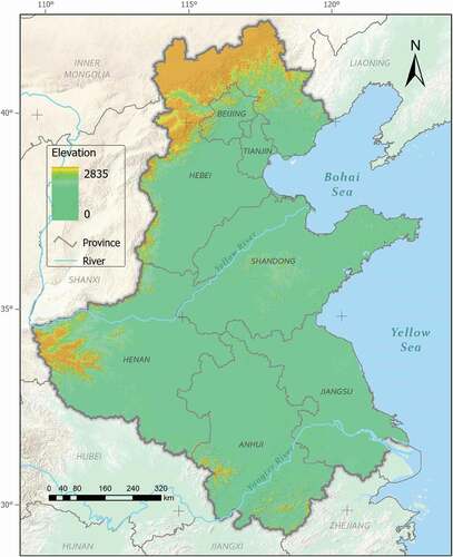
Five central and eastern provinces of China (i.e. Henan, Hebei, Shandong, Anhui, and Jiangsu) and two municipalities (i.e. Beijing and Tianjin), corresponding to the North China Plain region, were selected as the study area (Figure 1). The area spans 780,000 km² and is home to over 450 million people (National Bureau of Statistics of China 2019b). The study area is one of China’s most rapidly developing regions with the urbanization rate (excluding Beijing and Tianjin) tripling from ~20% in 1990 to ~60% in 2018 (National Bureau of Statistics of China 2019b). The North China Plain is key to China’s economic development and food security (Song and Deng 2015), generating ~37% of the gross domestic product and ~35% of China’s grain production in 2019 (National Bureau of Statistics of China 2019a). Managing the tension between rapid economic development, urbanization, and food production in the study area demands accurate quantification of built-up land dynamics to support policy formulation and decision making (Li et al. 2020a; Liu et al. 2020).

Figure 1. Map of the North China Plain

Method overview

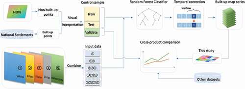
The approach taken in this study is summarized in Figure 2. Due to its high computational performance and vast historical satellite imagery archive, Google Earth Engine was used to process all remotely sensed data and map built-up land (Gorelick et al. 2017). Control points were visually checked using Landsat images from 1990–1992 and Google Earth high-definition images (from GeoEye, WorldView, SPOT, and Pleiades) from 2014 and 2019. We randomly withheld 25% of the control points as validation samples. Cloud-free Spectral images, normalized Indices (e.g. NDVI), Fourier predictors (e.g. Fourier transformation coefficients), Terrain, and Meteorological data were sequentially added to a Random Forest (RF) classifier to assess the additional benefit for classification accuracy. A temporal correction algorithm was then applied to remove inconsistent classifications. Lastly, a cross-product comparison was carried out using the withheld control points.

Figure 2. Flowchart outlining the methods used to map built-up land in the North China Plain. The National Settlements Database stores the geographic coordinates of government departments and state-owned companies in 2000 (http://www.resdc.cn/). The Spectral data refers to the cloud-free image produced from the Landsat data. Indices variables refer to the normalized difference vegetation index (NDVI), enhanced vegetation index (EVI), and normalized difference built-up index (NDBI). The Fourier predictors are coefficients derived from a discrete Fourier transformation on the Indices data (NDVI, NDBI, and EVI). Terrain data were a digital elevation model and slope derived from the Shuttle Radar Topography Mission. Meteorology data were taken from the China Meteorological Forcing Dataset (http://data.tpdc.ac.cn/)

Data and input predictors

We used five types of remotely sensed data as predictors to map built-up areas (Table 1). Spectral predictors comprised cloud-free images computed from Landsat and Sentinel 2A. Indices predictors were calculated from Landsat cloud-free data, including the NDVI, enhanced vegetation index (EVI), and normalized difference built-up index (NDBI). The Fourier predictors were derived from the Discrete Fourier Transformation of dense time-stacks of Indices data (NDVI, NDBI, and EVI). Lastly, Terrain data was taken from the Shuttle Radar Topography Mission and the Meteorology data was taken from the China Meteorological Forcing Dataset (He et al. 2020). The Landsat and Sentinel data were subject to geometric and radiometric corrections by Google Earth Engine, and all data were resampled to 30 m resolution for use in the classification.

Table 1. Input predictors for built-up land mapping. TM: Thematic Mapper, ETM+: Enhanced Thematic Mapper Plus, OLI: Operational Land Imager, MSI: Multispectral Instrument, NDVI: normalized difference vegetation index, EVI: enhanced vegetation index, and NDBI: normalized difference built-up index. All bands of the Landsat/Sentinel are used in this research. Note the panchromatic band (15 m resolution) of Landsat ETM+ and OLI, and the thermal bands (which have a resolution of 60 m for Landsat5/7 and 100 m for Landsat 8) are resampled to 30 m. All Sentinel bands are resampled to 30 m

Input type	Source	Spatial resolution	Number of bands	Years
Spectral	Landsat TM	30 m	7	1990–2010
	Landsat ETM+	30 m	9	2011–2013
	Landsat OLI	30 m	11	2014–2019
	Sentinel-2A MSI	10 m	13	2015–2019
Indices	NDVI	30 m	1	1990–2019
	EVI	30 m	1	1990–2019
	NDBI	30 m	1	1990–2019
Fourier	Coefficients of the Discrete Fourier Transformation	30 m	24	1990–2019
Meteorology	China Meteorological Forcing Data (Annual product)	0.1°	7	1990–2018
Terrain	Elevation	30 m	1	1990–2019
	Slope	30 m	1	1990–2019

The Spectral predictors were cloud-free images produced from Landsat and Sentinel-2A; the data quantity and distribution can be seen in Supplementary Material A (Figure SA 1). Spectral predictors were created using the simpleComposite module in Google Earth Engine. For each pixel in the collection of Landsat images, this module assigned a cloud score (0–100) to it and used the median value from pixels with a cloud score <10 to create a cloud-free image. For the Sentinel 2 Multi-Spectral Instrument (MSI) data, its Quality Assessment band that indicates whether the pixel is covered by cloud and cirrus was used to remove cloudy pixels, and the median value of the remaining pixels was mosaicked to create the Spectral predictors.

NDVI, EVI, and NDBI were selected as Indices predictors because NDVI and EVI are robust for delineating land covers (Li, Gong, and Liang 2015), and NDBI suits the purpose of built-up mapping (Li et al. 2018). We calculated these indices as follows:

(1) $NDVI=\left(NIR-R\right)/\left(NIR+R\right)$(1)

(2) $EVI=2.5\times \left(\left(NIR-R\right)/\left(NIR+6\times R-7.5\times B+1\right)\right)$(2)

(3) $NDBI=\left(SWIR1+NIR\right)/\left(SWIR1-NIR\right)$(3)

where NIR refers to the near-infrared band, R refers to the red band, B refers to the blue band, and SWIR1 refers to the first shortwave infrared band.

The Discrete Fourier Transformation approximates a series of discrete values by summing up a linear function and several pairs of sinuate functions. The fitting formulation was as follows:

(4) $p_t={\beta }_0+{\beta }_{1}t+\sum _{k=1}^n[{\alpha }_{\mathrm{k}}\mathrm{c}\mathrm{o}\mathrm{s}\left(2\pi \mathrm{k}\omega t\right)+{\theta }_{\mathrm{k}}\mathrm{s}\mathrm{i}\mathrm{n}\left(2\pi \mathrm{k}\omega t\right)]+e_t$(4)

where $t$ is the time difference in year fractions compared to 1970 following standard practice in data science, $p_t$ is the pixel value at time t, $n$ is the number of sinuate function pairs, ${\beta }_0$ and ${\beta }_1$ are the coefficients of the linear function, ${\alpha }_{\mathrm{k}}$ and ${\theta }_{\mathrm{k}}$ are the sinuate coefficients, $\omega$ is the frequency, and $e_t$ is the error between the actual observation and the fitted value.

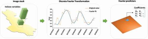
In practice, n and the temporal interval were the two variables that should be determined before the fitting. We assessed the impact of different n and temporal intervals from 1 to 5 and selected 3 for both variables because they did not unduly increase the fitting error (Figure SA 3). Meanwhile, we selected ω = 1 based on the climate and vegetation life-cycle and seasonality in the study area (Tang et al. 2020). Discrete Fourier Transformation was applied to the normalized indices to generate Fourier predictors (Figure 3). Eight coefficients were generated per index, and 24 coefficient bands were created as Fourier predictors.

Figure 3. The discrete fourier transformation of stacked indices data. coefficients of the fitting function were derived as fourier predictors

The China Meteorological Forcing Dataset (http://data.tpdc.ac.cn/) and Shuttle Radar Topography Mission data were incorporated as additional predictors to reduce interference of different climatic and topographic conditions. The China Meteorological Forcing Dataset includes seven variables: temperature (K), air pressure (Pa), specific humidity (kg kg⁻¹), wind speed (m s⁻¹), downward shortwave radiation (W m⁻²), downward longwave radiation (W m⁻²), and precipitation (mm yr⁻¹). The Shuttle Radar Topography Mission data used in this study included elevation and slope from the year 2000.

Built-up land mapping

Control point collection

Control points were collected manually via visual interpretation against high-resolution imagery and Indices images. Built-up and non-built-up control points were collected separately. Raw built-up points were taken from the National Settlements Database of China (http://www.resdc.cn/). Raw non-built-up points were generated via stratified sampling using NDVI (Figure SB 1). A total of 8,000 control points were verified, with an equal number of built-up and non-built-up points (i.e. 4,000) to reduce bias caused by uneven sample distribution (Stehman and Foody 2019). We took advantage of the irreversibility of built-up land (i.e. built-up land rarely reverts to non-built-up land) to ensure that control points were located in areas where land-use remained stable over time. We used the Indices image for the first period (1990–1992) to verify built-up control points, and the high-definition Google Earth images in the last period (2020) to verify non-built-up control points. We then merged the verified control points for use in classification throughout the analysis period (1990–2019). A sensitivity test showed that using more than 50% of control samples achieved high accuracies that were stable over time (Figure SC 1). Hence, we used 75% of control samples as the training sample for the mapping (of these, 70% were employed in classification and 30% to calculate accuracy), while the remaining ~25% were held out as validation samples for the cross-product comparison.

Classifying built-up land

Random Forest (RF) is an ensemble learning algorithm selected for classification due to its flexibility in capturing non-linear patterns between independent and dependent variables (Calderón-Loor, Hadjikakou, and Bryan 2021). The tree-based structure of RF is efficient in classifying high-dimensional data (Wang, Azzari, and Lobell 2019). To grow trees for the RF, we set the split nodes as the square root of the input predictors, the bag fraction to 50%, and the minimum leaf nodes to 1. The number of trees in the RF was set to 100 because no more improvement was possible by increasing tree numbers (Figure SC 1).

The input predictors were resampled to 30 m resolution and stacked into a single multi-band image in the classification process. The control samples were overlayed upon this image to extract values for each band. These samples were then used to train the RF model. Lastly, the trained model was used to map the spatial distribution of built-up land pixels (allocated a value of 1) versus non-built-up land pixels (allocated a value of 0) based on the input predictor bands.

All five types of predictors used in mapping were introduced in the following order: Spectral, Indices, Fourier, Terrain, Meteorology. The incorporation of predictors in this order enabled us to explore how temporal features improved built-up land mapping over the more traditional inputs. We first applied the traditional approach of using Spectral data only, then introduced the Indices data, then the Fourier predictors. Terrain and Meteorology data were added last to reduce interference from topographic and climatic conditions.

We classified built-up land using a random selection of control points and repeated this ten times to eliminate bias and capture uncertainty in accuracy metrics. In each classification, 70% of the training samples were randomly selected to train the RF classifier, and the remaining 30% were used to compute overall accuracy. Uncertainty was then calculated as the standard error of the accuracies of the ten simulations. We summed the 10 classifications and identified the built-up land pixels as the pixels with >4 value to derive the final classification of built-up land. Four was chosen as the threshold because it led to the highest classification accuracy (Figure SC 2).

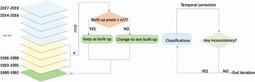
Based on the characteristic of the irreversibility of built-up land development and expansion (Gong et al. 2020; Li, Gong, and Liang 2015), we constructed temporal check rules to correct inconsistent pixel classifications over time (Figure 4). Irreversibility was implemented as a check rule such that built-up land extent in earlier years could not expand beyond the built-up land extent mapped in later years. For each built-up land pixel in the map, n subsequent pixels in the later years were used to check its consistency: if >n/2 of the subsequent pixel were classified as a built-up land, the pixel remained as built-up land; otherwise, it was corrected and specified as non-built-up land. The >n/2 threshold was based on a “majority vote” rule (Li, Gong, and Liang 2015). This study set n = 2 by balancing the amount of data used as a mask and the resulting improvements in accuracy (Figure SD 1). The temporal correction process was iterated eight times to ensure consistency (Figure SD 2).

Figure 4. Temporal correction for built-up land mapping. Left, the temporal correction process for each iteration; right, the stop condition of the iteration. Here we choose n = 2 based on a sensitivity test (Figure SD 1)

Cross-product comparison

We compared our data to other datasets available for the study area that mapped similar land cover (such as impervious surfaces and human settlements) or including urban/built-up land (Table 2). Built-up area and overall accuracy were used for the comparison. The validation sample (25% of all control samples) was used to compute overall accuracy because it was not used in the original classification of this study, thereby eliminating bias from the comparison (Stehman and Foody 2019). The other data products tended to be global in coverage. In this sense, our aim was not to critically compare our dataset explicitly which was created for the study area against global datasets (which is an unfair comparison), but rather to provide a guide for potential users (i.e. planners, policy-makers) of the accuracy of our product compared to other available products for this specific region and to provide a basis for understanding the potential implications in terms of the urban land area mapped.

Table 2. Global built-up land datasets used for comparison with the outputs of this study. GAIA: Global Artificial Impervious Area, ESA CCI: European Space Agency Climate Change Initiative, GHSL: Global Human Settlement Layer, MCD12Q1: MODIS Land Cover Type Product, MERIS: Medium-spectral Resolution Imaging Spectrometer, SPOT-VGT: Strategic Planning Online Tool Vegetation Instrument, PROBA-V: Project for On-Board Autonomy Vegetation, AVHRR: Advanced Very High-Resolution Radiometer, and MODIS: Moderate Resolution Imaging Spectroradiometer

Dataset	Sensors	Resolution	Timeframe	Source
GAIA	Landsat TM/ETM+/OLI, Sentinel-1&2, VIIRS NTL	30 m	Annual map 1985–2018	Gong et al. 2020
ESA CCI	MERIS, SPOT-VGT, PROBA-V AVHRR	300 m	Annual map 1992–2015	Buchhorn et al. 2020
GHSL	Landsat TM/ETM+/OLI	38 m	1975, 1990, 2000, 2014	Corbane et al. 2018
Global Urban Dynamics	Landsat, VIIRS NTL	30 m	1990, 1995, 2000, 2005, 2010, 2015	Liu et al. 2019
Global Urban Expansion	VIIRS NTL, MODIS	1000 m	1992, 1996, 2000, 2006, 2010, 2016	He et al. 2019
MCD12Q1	MODIS	500 m	Annual map 2001–2019	Friedl and Sulla-Menashe 2019
Global Impervious Surface	Landsat, Sentinel	30 m	2015	Zhang et al. 2020
GlobeLand30	Landsat TM/ETM+/OLI, Gaofen-1	30 m	2000, 2010, 2020	Jun, Ban, and Li 2014

Results

Built-up land mapping using different predictors

The performance of different predictors is shown in Figure 5. The mapping accuracy of 2014–2016 and 2017–2019 were significantly higher because the Sentinel-2A MSI data was incorporated in the classification, increasing classification accuracy from ~83% in 2011–2013 to ~93% in 2017–2019. Fourier and Indices were the best predictors, increasing accuracy by ~8% and ~3%, respectively. The addition of Terrain and Meteorology predictors further improved the mapping accuracy by ~1%.

Figure 5. Accuracy of different predictor combinations for built-up land mapping. Lines show the median value of 10 classifications with varying sample splits; the margins show the standard error

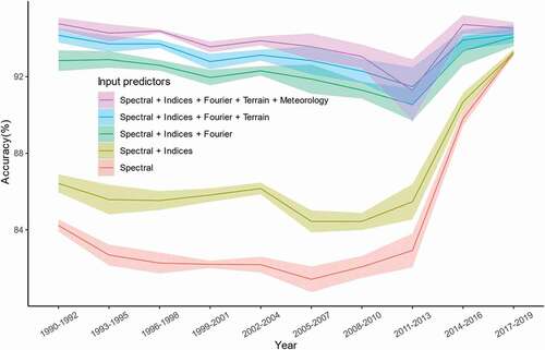
For classifications in the 1990s and 2000s, incorporating the Fourier predictors raised the overall accuracy to ~92%, similar to the overall accuracy in 2014–2019 achieved using Sentinel-2A MSI data. Hence, incorporating Fourier predictors for the earlier time periods (Landsat 5 TM or Landsat 7 ETM+) enabled the mapping of built-up land with an accuracy similar to the classification based on data sourced from more recent and more advanced sensors (i.e. Landsat 8 OLI and Sentinel-2A MSI).

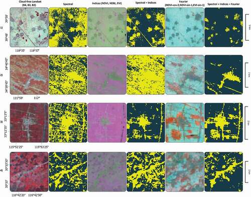
Built-up land mapping for the period 1990–1992 was selected to explore the spatial performance of Spectral, Indices, and Fourier predictors (Figure 6). Region 1 (row 1, Figure 6) shows villages surrounded by farmland, where the classification using Spectral predictors misclassified large areas of farmland near villages as built-up land. Region 2 (row 2, Figure 6) shows a town surrounded by bare lands. The classification using Spectral predictors misclassified most bare land to build-up land. Regions 3 and 4 (rows 3 and 4, Figure 6) were located in more humid areas than regions 1 and 2. Figure 6 shows that bare lands and farmland rotation confounded built-up land mapping. The addition of Indices predictors reduced misclassification in Regions 1 and 3 but worsened the classification in regions 2 and 4. However, the Fourier predictors provided skilled delineation of built-up land mapping across the four example regions.

Figure 6. Spatial improvement in built-up land mapping for four selected regions. We used a false-color composite scheme to display predictors and a two-color map to represent the classification results (with yellow indicating built-up land and the dark color non-built-up). Regions 1 and 2 were located in the northern, temperate part of the study area; regions 3 and 4 were located in the more humid southern part. NDVI-cos-2, NDVI-sin-1, and EVI-sin-1 are selected to present the Fourier predictors to give maximum visual contrast to built-up land. NDVI-cos-2 refers to the cosine coefficient with a frequency of 2 from the Fourier transformation on NDVI. NDVI-sin-1 and EVI-sin-1 are the sine coefficients with a frequency of 1

Accuracy improvements via temporal correction

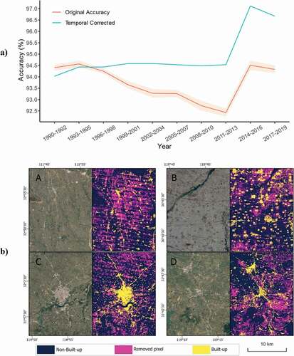
Figure 7a shows classification accuracy before and after temporal correction. Temporal correction increased built-up land classification accuracy, achieving consistently high accuracies over the entire study period. The highest accuracy increases (1.5%–2.5%) occurred in the last two periods, while the accuracy of the first two periods decreased by 0.1%–0.5%. We further inspected spatial improvements in 2011–2013 because the classification in this period had the lowest original accuracy (Figure 7b). The temporal correction process greatly reduced misclassification of the striping in the original imagery created by the Scan-Line Corrector failure of Landsat ETM+ (regions A and C), correctly removed erroneously classified greenhouses (hazy, light gray patches in region B), and improved classification quality in hilly and barren areas (region D).

Figure 7. Improvement in overall accuracy and spatial performance when using temporal correction. true-color maps in b) were obtained from high-definition Google Earth imagery from December 2013

Spatio-temporal dynamics of built-up land

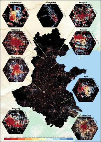
We mosaicked all temporally corrected classifications into one image and used a warm-cool color scheme to represent time from 1990 to 2019 (Figure 8). Cities in flatter regions (e.g. Baoding, Shangqiu, and Changzhou) tended to expand radially outward. Cities near rivers (e.g. Xuyi and Xinyang) grew linearly following the geographical constraints, and cities in mountainous areas (e.g. Fengning) expanded along valleys.

Figure 8. Dynamic map of built-up areas from 1990 to 2019. Warm colors indicate earlier dates, and cool colors indicate later dates. Hexagonal insets show zoomed-in views of selected cities

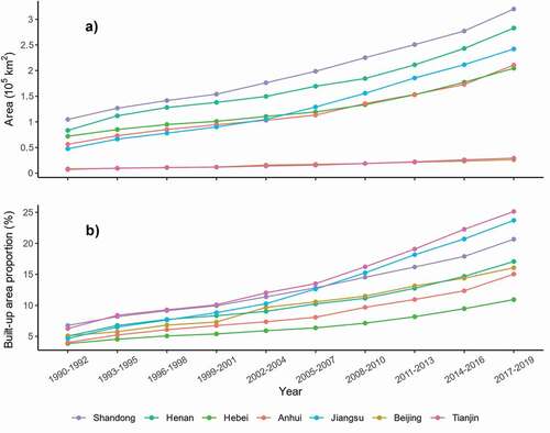
The increase in built-up area accelerated over the study period, with all provinces, except for Hebei, tripling their built-up area (Figure 9). Shandong and Henan provinces had the largest built-up area. Jiangsu province rose from the fifth-largest built-up land area to the third after 2004, while Hebei and Anhui had less built-up land area. Beijing and Tianjin showed similar amounts of built-up land area for all periods and both increased rapidly. Tianjin demonstrated the largest change in proportion of built-up land, expanding from 6.3% in 1990–1992 to 25.1% in 2017–2019. The ratio of built-up land increased from 4.7% to 23.7% in Jiangsu and from 8.2% to 20.6% in Shandong. Henan, Beijing, and Anhui shared a comparable growth level of ~5% to ~16%. Hebei demonstrated the lowest concentration of built-up land, increasing from 3.8% in 1990–1992 to 10.9% in 2017–2019.

Figure 9. Built-up land change in the North China Plain from 1990 to 2019. a) The area change. b) The built-up area proportion change; the value shows the percentage of built-up area to region total area

Cross-product comparison

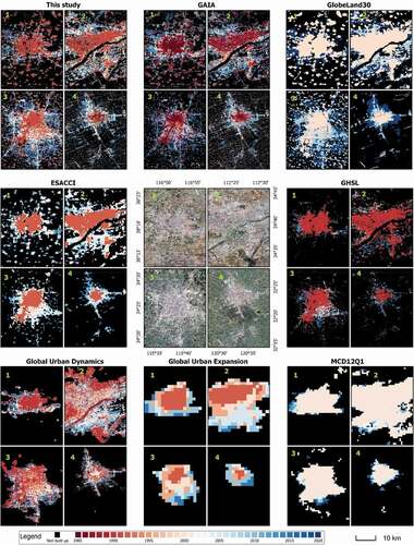
Significant differences were found between the selected datasets because of the differences in classification algorithms, data sources, spatial resolution, and definitions used (Figure 10). The low-resolution datasets (ESA CCI, Global Urban Expansion, and MCD12Q1) missed built-up land in smaller villages and towns. The Global Urban Dynamics used Landsat imagery as input data and the VIIRS NTL as a mask to map the urban land dynamics but omitted small villages/towns that emit faint nighttime light. However, the GAIA product more skillfully captured built-up land in large cities and smaller villages and towns.

Figure 10. Dynamics of built-up area in four selected cities (1990–2019). The true color maps were taken from Google Earth high-definition images from 2019. GAIA: Global Artificial Impervious Area, ESA CCI: European Space Agency Climate Change Initiative, GHSL: Global Human Settlement Layer, MCD12Q1: MODIS Land Cover Type Product. Note that the start year for GAIA was 1985, making its city centers look darker than our product

We further compared built-up areas and overall accuracy between our study and other datasets (Figure 11a). Our study computed the second-largest built-up area throughout the study period, similar to other high-resolution datasets (i.e. GAIA, GHSL, and GlobeLand30). In the 1990s, our built-up land estimates were in broad agreement with GAIA and GHSL but were significantly higher than ESA CCI, Global Urban Dynamics, and Global Urban Expansion. GAIA, ESA CCI, and our data showed an acceleration in built-up area expansion, while GHSL, MODIS, Global Urban Dynamics, and the Global Urban Expansion showed linearly increasing trends.

Figure 11. Area and overall accuracy comparison. The middle year of each period in this study was selected as the x-axis value (for example, 1991 was used to indicate the built-up area of 1990–1992)

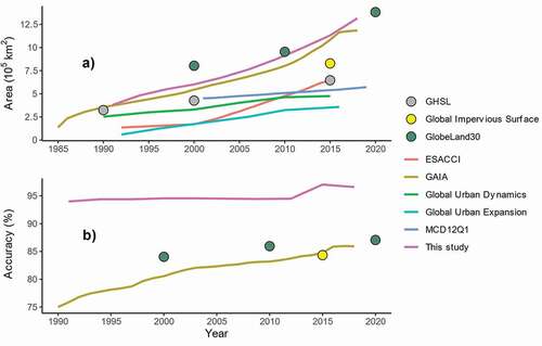
Due to their similar spatial resolution and land-cover definition, GAIA, Global Impervious Surface, and GlobeLand30 were selected for the accuracy comparisons. The accuracy of our study was 10% higher than GHSL and Global Impervious Surface, and 10–19% higher than GAIA, especially in the earlier years. Our accuracy was consistently high (>94%) across all years, while that of the Global Impervious Surface and GlobeLand30 were ~85%, and GAIA’s accuracy ranged from 75% in 1990 to 84% in 2017.

Discussion

Fourier predictors improved built-up land mapping accuracy

Landsat has a long and continuous image archive which offers a unique opportunity for global and regional assessment of land-use change processes such as urbanization (Deng and Zhu 2020). However, fallow farmland and seasonal bare land introduce confusion into built-up land mapping (Gong et al. 2020; Poursanidis, Chrysoulakis, and Mitraka 2015). This study used coefficients from a Discrete Fourier Transformation as predictors and achieved an 8% accuracy gain compared to using traditional Spectral and Indices-based approaches. Fallow farmland and seasonal bare land confusion were largely removed following the inclusion of Fourier predictors. Our results captured fine-scale built-up features, such as buildings in small villages and towns, rather than just the large-scale features of large cities. As a result of the higher accuracy, our study revealed higher estimates of built-up areas than other datasets (except for GlobeLand30), suggesting that global assessments of urbanization may be underestimated.

The effectiveness of Fourier predictors in delineating built-up lands may be because features captured in dense time-stacks of remotely sensed data are less affected by random noise (e.g. cloud, cloud shadow, and seasonal changes in land surface) than snapshot spectral data or indices. Crop phenology and farming rotations lead to regular greenness patterns in cultivated sites over the annual growing cycle that are distinct from built-up lands (Zeng et al. 2020). While it is difficult for Spectral and Indices predictors to separate fallow lands from built-up lands – a common source of built-up land mapping error – Fourier predictors were sensitive to this distinction. Incorporating Fourier predictors reduced this confusion and substantially increased the accuracy of built-up land mapping.

Temporal correction increases the consistency of long time-series built-up land mapping

In addition to incorporating Fourier predictors, we also implemented temporal correction to account for the general feature of irreversibility in built-up land (i.e. once an area is converted to urban land, it tends to remain as urban land (Li, Gong, and Liang 2015; Li et al. 2018)). We implemented the rule that built-up land in earlier years was unlikely to occur beyond the extent of built-up land in later years, providing the logic for developing a temporal correction algorithm to remove incorrect pixel classifications. This correction was able to remove misclassified areas resulting from striping caused by the ETM+ Scan-Line Corrector failure. Our method can be deployed on the Google Earth Engine platform and is more straightforward than other temporal correction algorithms. For example, Li, Gong, and Liang (2015) combined a majority vote rule and temporal reasoning to construct a spatio-temporal consistency check algorithm, which required a complicated process to combine transition probabilities and neighborhood characteristics. In comparison, our heuristic method is straightforward to apply and achieved a significant correction effect.

Combining Fourier predictors and temporal correction achieved consistently high accuracy in built-up land mapping over 30 years. The overall accuracy of our product was high and consistent across years (>94%), averaging around ~10% higher than the GlobeLand30 and ~15% higher than GAIA in the 1990s and 2000s (Figure 11).

Informing sustainability assessment and supporting policy with high-quality data

Built-up land occupies only a small portion of the global terrestrial surface but hosts more than half of the world’s population (Chen et al. 2020). Indeed, 70% of global anthropogenic greenhouse gas emissions in 2016 and 80% of local natural habitat loss in 2018 have been linked to the development of built-up lands (Hopkins et al. 2016; Ke et al. 2018). Therefore, an accurate understanding of the dynamics of built-up land over time is critical to addressing the social and environmental challenges that threaten a sustainable future in rapidly urbanizing areas, including our study area.

Our consistent, high-accuracy data product can be readily used in urban policy and planning. For example, urban growth models based on cellular automata use historical data to project future scenarios, but errors in historical data can propagate throughout the projection, reducing confidence in the results (Clarke and Johnson 2020; Roodposhti, Aryal, and Bryan 2019). This study provides reliable historical data that enables built-up land expansion to be projected with higher confidence. Environmental change can also be quantified more precisely using accurate built-up land maps. For example, the Integrated Valuation of Ecosystem Services and Trade-offs (InVEST) model uses land-use maps as a proxy to calculate carbon sequestration, water yield, crop production, and habitat quality (Tallis et al. 2011). High-quality built-up land mapping data can provide more reliable input data for calculating the anthropogenic impacts of urbanization.

Spatially explicit policies and planning are essential for supporting sustainable development, and one requirement for formulating such policies is access to high-quality data. The study area is unique in China for its strategic position, rapid urbanization, and high agricultural productivity (Song and Deng 2015). To boost the economy of the study area, the Chinese government has announced a series of development plans, such as the Beijing-Tianjin-Hebei Urban Agglomeration development plan (Fang et al. 2019) and the Central Plains City Group development plan (Li et al. 2020a). These plans include mega-infrastructure projects (e.g. high-speed railways and long-distance expressways) to enhance economic flow among cities (Li et al. 2020a). In parallel, to safeguard food security, the Chinese government has also enacted strict farmland protection regulations (e.g. the Basic Farmland Protection Regulations) that prohibit farmland from being converted to built-up lands (Liu et al. 2020). An accurate understanding of built-up land dynamics is critical to formulating effective development plans that balance rapid urbanization with increased demand for food production (Zhong et al. 2020). In addition, accurate historical built-up data can be used to project future economic development and derive opportunity costs for future urban expansion (e.g. reduced food security). As a result, urbanization, food security, and sustainability can be coordinated under one framework, promoting the formulation of spatially explicit policies and regulations.

Limitations and prospects

Our study has some limitations and uncertainties. We derived temporal features from the Discrete Fourier Transformation based on three years of data. Hence the exact date of built-up land development cannot be determined at a finer resolution than three years. Another uncertainty was introduced by the temporal correction methodology, which assumes that built-up land in 1990–1992 remained unchanged during the study period. Small areas of built-up land could have been converted to other land types over time (Fu et al. 2019). However, such conversions typically only comprise a small portion of the total built-up land area (Gong, Li, and Zhang 2019). Despite these limitations, the results provide the most accurate, high-resolution, long time-series built-up land data product available for the North China Plain.

The cross-product comparison indicates that our built-up land mapping for the North China Plain is more consistent and accurate than other available products that map built-up land. However, while comparing the accuracy of highly-tailored, regional mapping applications against other global datasets enables potential users to evaluate the merits of the products available for a specific region; it is not a reflection on the value of the global datasets as the accuracy of global products is bound to be lower. Our dataset fills a different niche, aimed at users that require consistent, high-accuracy, long-time series data for a specific region rather than global coverage.

Conclusion

We incorporated temporal features based on a dense time-stack of Landsat imagery and a temporal correction method to map the spatial extent of built-up land in the North China Plain over 30 years (1990–2019). Incorporating Fourier predictors increased overall accuracy by 8% compared to using Spectral and Indices predictors alone. The temporal correction successfully removed incorrectly classified pixels and increased overall accuracy in all periods to a consistently high level (>94%). All provinces and cities in the study region tripled their built-up area over the last three decades, illustrating the fierce competition between urban and agricultural land uses. Consistent, high-accuracy and long time-series mapping of built-up land is invaluable for helping to understand recent patterns of rapid urbanization, quantifying impacts for food security and the environment, modeling future land-use change, and informing policy and planning for managing future urbanization and sustainable development.

Acknowledgements

We thank Lauren McManus who visually interpreted the control points.

Data and codes availability statement

The data and codes that support the findings of this study are available at GitHub (https://github.com/wangjinzhulala/North_China_Plain_GEE_Organized).

Disclosure statement

No potential conflict of interest was reported by the author(s).

Additional information

Funding

A Deakin University Postgraduate Research scholarship funded this research.

References

- Brown, L. R. 1997. Who Will Feed China? Wake-up Call for a Small Planet. Vol. 5. New York: WW Norton & Company.
- Bryan, B. A., Y. Yanqiong, J. Zhang, and J. D. Connor. 2018. “Land-use Change Impacts on Ecosystem Services Value: Incorporating the Scarcity Effects of Supply and Demand Dynamics.” Ecosystem Services 32: 144–157. doi:https://doi.org/10.1016/j.ecoser.2018.07.002.
- Buchhorn, M., M. Lesiv, N.-E. Tsendbazar, M. Herold, L. Bertels, and B. Smets. 2020. “Copernicus Global Land Cover Layers—Collection 2.” Remote Sens 12 (6): 1044. doi:https://doi.org/10.3390/rs12061044
- Calderón-Loor, M., M. Hadjikakou, and B. A. Bryan. 2021. “High-resolution Wall-to-wall Land-cover Mapping and Land Change Assessment for Australia from 1985 to 2015.” Remote Sens. Environ 252: 112148. doi:https://doi.org/10.1016/j.rse.2020.112148.
- Cao, S., H. Deyong, W. Zhao, M. You, Y. Chen, and Y. Zhang. 2019. “Monitoring Changes in the Impervious Surfaces of Urban Functional Zones Using Multisource Remote Sensing Data: A Case Study of Tianjin, China.” GIScience & Remote Sensing 56 (7): 967–987. doi:https://doi.org/10.1080/15481603.2019.1600110.
- Chai, B., and L. Peijun. 2018. “Annual Urban Expansion Extraction and Spatio-Temporal Analysis Using Landsat Time Series Data: A Case Study of Tianjin, China.” IEEE J. Sel. Top. Appl. Earth Obs. Remote Sens 11 (8): 2644–2656. doi:https://doi.org/10.1109/JSTARS.2018.2829525.
- Chen, G., L. Xia, X. Liu, Y. Chen, X. Liang, J. Leng, X. Xiaocong, et al. 2020. “Global Projections of Future Urban Land Expansion under Shared Socioeconomic Pathways.” Nature Communications 11 (1): 537. doi:https://doi.org/10.1038/s41467-020-14386-x.
- Chen, J., P. Jönsson, M. Tamura, Z. Gu, B. Matsushita, and L. Eklundh. 2004. “A Simple Method for Reconstructing A High-quality NDVI Time-series Data Set Based on the Savitzky–Golay Filter.” Remote Sensing of Environment 91 (3–4): 332–344. doi:https://doi.org/10.1016/j.rse.2004.03.014.
- Christina, A. F., M. Pesaresi, P. Politis, and V. Syrris. 2018. “GHS Built-up Grid, Derived from Landsat, Multitemporal (1975-1990-2000-2014), R2018A.” doi:https://doi.org/10.2905/JRC-GHSL-10007./rs12061044
- Clarke, K. C., and J. M. Johnson. 2020. “Calibrating SLEUTH with Big Data: Projecting California’s Land Use to 2100.” Computers, Environment and Urban Systems 83: 101525. doi:https://doi.org/10.1016/j.compenvurbsys.2020.101525.
- de Beurs, K. M., and G. M. Henebry. 2004. “Land Surface Phenology, Climatic Variation, and Institutional Change: Analyzing Agricultural Land Cover Change in Kazakhstan.” Remote Sens. Environ 89 (4): 497–509. doi:https://doi.org/10.1016/j.rse.2003.11.006.
- Deng, C., and Z. Zhu. 2020. “Continuous Subpixel Monitoring of Urban Impervious Surface Using Landsat Time Series.” Remote Sens. Environ 238: 110929. doi:https://doi.org/10.1016/j.rse.2018.10.011.
- Elmore, A. J., S. M. Guinn, B. J. Minsley, and A. D. Richardson. 2012. “Landscape Controls on the Timing of Spring, Autumn, and Growing Season Length in mid-Atlantic Forests.” Global Change Biol 18 (2): 656–674. doi:https://doi.org/10.1111/j.1365-2486.2011.02521.x.
- Fang, C., X. Cui, L. Guangdong, C. Bao, Z. Wang, M. Haitao, S. Sun, H. Liu, K. Luo, and Y. Ren. 2019. “Modeling Regional Sustainable Development Scenarios Using the Urbanization and Eco-Environment Coupler: Case Study of Beijing-Tianjin-Hebei Urban Agglomeration, China.” The Science of the Total Environment 689: 820–830. doi:https://doi.org/10.1016/j.scitotenv.2019.06.430.
- Filazzola, A., N. Shrestha, J. S. MacIvor, and M. Stanley. 2019. “The Contribution of Constructed Green Infrastructure to Urban Biodiversity: A Synthesis and Meta‐analysis.” Journal of Applied Ecology 56 (9): 2131–2143. doi:https://doi.org/10.1111/1365-2664.13475.
- Foga, S., P. L. Scaramuzza, S. Guo, R. D. Zhe Zhu, T. B. Dilley, G. L. Schmidt, J. L. Dwyer, L. Brady, B. Laue, and B. Laue. 2017. “Cloud Detection Algorithm Comparison and Validation for Operational Landsat Data Products.” Remote Sensing of Environment 194: 379–390. doi:https://doi.org/10.1016/j.rse.2017.03.026.
- Friedl, M., D. Sulla-Menashe. 2019. “MCD12Q1 MODIS/Terra+Aqua Land Cover Type Yearly L3 Global 500m SIN Grid V006. 2019, distributed by NASA EOSDIS Land Processes DAAC.” doi:https://doi.org/10.5067/MODIS/MCD12Q1.006
- Fu, Y., L. Jiufeng, Q. Weng, Q. Zheng, S. D. Le Li, B. Guo, and B. Guo. 2019. “Characterizing the Spatial Pattern of Annual Urban Growth by Using Time Series Landsat Imagery.” Science of the Total Environment 666: 274–284. doi:https://doi.org/10.1016/j.scitotenv.2019.02.178.
- Gong, P., L. Xuecao, J. Wang, Y. Bai, B. Chen, H. Tengyun, X. Liu, et al. 2020. “Annual Maps of Global Artificial Impervious Area (GAIA) between 1985 and 2018.” Remote Sens. Environ 236. doi:https://doi.org/10.1016/j.rse.2019.111510.
- Gong, P., L. Xuecao, and W. Zhang. 2019. “40-Year (1978–2017) Human Settlement Changes in China Reflected by Impervious Surfaces from Satellite Remote Sensing.” Sci. Bull. (Science Bulletin) 64 (11): 756–763. doi:https://doi.org/10.1016/j.scib.2019.04.024.
- Gorelick, N., M. Hancher, M. Dixon, S. Ilyushchenko, D. Thau, and R. Moore. 2017. “Google Earth Engine: Planetary-scale Geospatial Analysis for Everyone.” Remote Sensing of Environment 202: 18–27. doi:https://doi.org/10.1016/j.rse.2017.06.031.
- Guo, W., L. Guiying, N. Wenjian, Y. Zhang, and L. Dengsheng. 2018. “Exploring Improvement of Impervious Surface Estimation at National Scale through Integration of Nighttime Light and Proba-V Data.” GIScience & Remote Sensing 55 (5): 699–717. doi:https://doi.org/10.1080/15481603.2018.1436425.
- He, C., Z. Liu, S. Gou, Q. Zhang, J. Zhang, and X. Linlin. 2019. “Detecting Global Urban Expansion over the Last Three Decades Using a Fully Convolutional Network.” Environmental Research Letters 14 (3): 3. doi:https://doi.org/10.1088/1748-9326/aaf936.
- He, J., K. Yang, W. Tang, L. Hui, J. Qin, Y. Chen, and L. Xin. 2020. “The First High-Resolution Meteorological Forcing Dataset for Land Process Studies over China.” Scientific Data 7 (1): 25. doi:https://doi.org/10.1038/s41597-020-0369-y.
- Hopkins, F. M., J. R. Ehleringer, S. E. Bush, R. M. Duren, C. E. Miller, C.-T. Lai, Y.-K. Hsu, V. Carranza, and J. T. Randerson. 2016. “Mitigation of Methane Emissions in Cities: How New Measurements and Partnerships Can Contribute to Emissions Reduction Strategies.” Earth’s Future 4 (9): 408–425. doi:https://doi.org/10.1002/2016ef000381.
- Hou, X., L. Feng, J. Tang, X.-P. Song, J. Liu, Y. Zhang, J. Wang, et al. 2020. “Anthropogenic Transformation of Yangtze Plain Freshwater Lakes: Patterns, Drivers and Impacts.” Remote Sensing of Environment 248 :111998. doi:https://doi.org/10.1016/j.rse.2020.111998.
- Jin, G., K. Chen, P. Wang, B. Guo, Y. Dong, and J. Yang. 2019. “Trade-offs in Land-use Competition and Sustainable Land Development in the North China Plain.” Technological Forecasting and Social Change 141: 36–46. doi:https://doi.org/10.1016/j.techfore.2019.01.004.
- Jönsson, P., Z. Cai, E. Melaas, M. Friedl, and L. Eklundh. 2018. “A Method for Robust Estimation of Vegetation Seasonality from Landsat and Sentinel-2 Time Series Data.” Remote Sensing 10 (4): 635. doi:https://doi.org/10.3390/rs10040635.
- Jun, C., Y. Ban, and S. Li. 2014. “China: Open Access to Earth Land-Cover Map.” Nature 514 (7523): 434. doi:https://doi.org/10.1038/514434c
- Ke, X., J. van Vliet, P. H. Ting Zhou, W. Z. Verburg, X. Liu, and X. Liu. 2018. “Direct and Indirect Loss of Natural Habitat Due to Built-up Area Expansion: A Model-based Analysis for the City of Wuhan, China.” Land Use Policy 74: 231–239. doi:https://doi.org/10.1016/j.landusepol.2017.12.048.
- Kuang, W., A. Liu, Y. Dou, L. Guiying, and L. Dengsheng. 2019. “Examining the Impacts of Urbanization on Surface Radiation Using Landsat Imagery.” GIScience & Remote Sensing 56 (3): 462–484. doi:https://doi.org/10.1080/15481603.2018.1508931.
- Lamb, W. F., F. Creutzig, M. W. Callaghan, and J. C. Minx. 2019. “Learning about Urban Climate Solutions from Case Studies.” Nature Climate Change 9 (4): 279–287. doi:https://doi.org/10.1038/s41558-019-0440-x.
- Li, G., C. Jiang, J. Du, Y. Jia, and J. Bai. 2020a. “Spatial Differentiation Characteristics of Internal Ecological Land Structure in Rural Settlements and Its Response to Natural and Socio-Economic Conditions in the Central Plains, China.” Science of the Total Environment 709: 135932. doi:https://doi.org/10.1016/j.scitotenv.2019.135932.
- Li, G., L. Longwei, L. Dengsheng, W. Guo, and W. Kuang. 2020b. “Mapping Impervious Surface Distribution in China Using Multi-Source Remotely Sensed Data.” GIScience & Remote Sensing 57 (4): 543–552. doi:https://doi.org/10.1080/15481603.2020.1744240.
- Li, S., F. A. Suzana Dragicevic, M. S. Castro, S. Winter, A. Coltekin, C. Pettit, C. Pettit, et al. 2016. “Geospatial Big Data Handling Theory and Methods: A Review and Research Challenges.” ISPRS Journal of Photogrammetry and Remote Sensing 115 (2): 119–133. doi:https://doi.org/10.1016/j.isprsjprs.2015.10.012.
- Li, X., and P. Gong. 2016. “An “Exclusion-inclusion” Framework for Extracting Human Settlements in Rapidly Developing Regions of China from Landsat Images.” Remote Sensing of Environment 186: 286–296. doi:https://doi.org/10.1016/j.rse.2016.08.029.
- Li, X., P. Gong, and L. Liang. 2015. “A 30-year (1984–2013) Record of Annual Urban Dynamics of Beijing City Derived from Landsat Data.” Remote Sensing of Environment 166: 78–90. doi:https://doi.org/10.1016/j.rse.2015.06.007.
- Li, X. C., Y. Y. Zhou, Z. Y. Zhu, L. Liang, B. L. Yu, and W. T. Cao. 2018. “Mapping Annual Urban Dynamics (1985-2015) Using Time Series of Landsat Data.” Remote Sensing of Environment 216: 674–683. doi:https://doi.org/10.1016/j.rse.2018.07.030.
- Liu, C., Q. Zhang, H. Luo, S. H. Qi, S. Q. Tao, H. Z. Y. Xu, and Y. Yao. 2019. “An Efficient Approach to Capture Continuous Impervious Surface Dynamics Using Spatial-Temporal Rules and Dense Landsat Time Series Stacks.” Remote Sensing of Environment 229: 114–132. doi:https://doi.org/10.1016/j.rse.2019.04.025.
- Liu, Y., L. Liu, A.-X. Zhu, C. Lao, H. Guohua, and H. Yueming. 2020. “Scenario Farmland Protection Zoning Based on Production Potential: A Case Study in China.” Land Use Policy 95: 104581. doi:https://doi.org/10.1016/j.landusepol.2020.104581.
- National Bureau of Statistics of China. 2019a. “Announcement of the 2019 Grain Output.” Accessed 20 December 2020 http://www.gov.cn/xinwen/2019-12/07/content_5459250.htm
- National Bureau of Statistics of China. 2019b. “China Statistical Yearbook.” Beijing: China Statistics Press. Accessed November 06: 2020.
- Nations, U. 2019. “World Urbanization Prospects 2018: Highlights.” Population Division, United Nations 32. doi:https://doi.org/10.18356/6255ead2-en.
- Odenweller, J. B., and K. I. Johnson. 1984. “Crop Identification Using Landsat Temporal-spectral Profiles.” Remote Sensing of Environment 14 (1–3): 39–54. doi:https://doi.org/10.1016/0034-4257(84).90006-3.
- Poursanidis, D., N. Chrysoulakis, and Z. Mitraka. 2015. “Landsat 8 Vs. Landsat 5: A Comparison Based on Urban and Peri-urban Land Cover Mapping.” International Journal of Applied Earth Observation and Geoinformation 35: 259–269. doi:https://doi.org/10.1016/j.jag.2014.09.010.
- Roodposhti, M. S., J. Aryal, and B. A. Bryan. 2019. “A Novel Algorithm for Calculating Transition Potential in Cellular Automata Models of Land-use/cover Change.” Environmental Modelling and Software 112: 70–81. doi:https://doi.org/10.1016/j.envsoft.2018.10.006.
- Schneider, A., and C. M. Mertes. 2014. “Expansion and Growth in Chinese Cities, 1978–2010.” Environmental Research Letters 9 (2): 24008. doi:https://doi.org/10.1088/1748-9326/9/2/024008.
- Shi, L., F. Ling, G. Yong, G. Foody, L. Xiaodong, L. Wang, Y. Zhang, and D. Yun. 2017. “Impervious Surface Change Mapping with an Uncertainty-Based Spatial-Temporal Consistency Model: A Case Study in Wuhan City Using Landsat Time-Series Datasets from 1987 to 2016.” Remote Sensing 9 (11): 1148. doi:https://doi.org/10.3390/rs9111148.
- Shrivastava, M., M. O. Andreae, H. M. Paulo Artaxo, J. Barbosa, L. K. Berg, J. Brito, J. Ching, et al. 2019. “Urban Pollution Greatly Enhances Formation of Natural Aerosols over the Amazon Rainforest.” Nature Communications 10 (1): 1046. doi:https://doi.org/10.1038/s41467-019-08909-4.
- Song, W., and X. Deng. 2015. “Effects of Urbanization-Induced Cultivated Land Loss on Ecosystem Services in the North China Plain.” Energies 8 (6): 5678–5693. doi:https://doi.org/10.3390/en8065678.
- Song, X. P., J. O. Sexton, C. Q. Huang, S. Channan, and J. R. Townshend. 2016. “Characterizing the Magnitude, Timing and Duration of Urban Growth from Time Series of Landsat-Based Estimates of Impervious Cover.” Remote Sensing of Environment 175: 1–13. doi:https://doi.org/10.1016/j.rse.2015.12.027.
- Stehman, S. V., and G. M. Foody. 2019. “Key Issues in Rigorous Accuracy Assessment of Land Cover Products.” Remote Sens. Environ 231. doi:https://doi.org/10.1016/j.rse.2019.05.018.
- Tallis, H. T., T. Ricketts, A. D. Guerry, E. Nelson, D. Ennaanay, S. Wolny, N. Olwero, K. Vigerstol, D. Pennington, and G. Mendoza. 2011. InVEST 2.1 Beta User’s Guide. The Natural Capital Project.California: Stanford.
- Tang, J., J. Zeng, Q. Zhang, R. Zhang, S. Leng, Y. Zeng, W. Shui, X. Zhanghua, and Q. Wang. 2020. “Self-Adapting Extraction of Cropland Phenological Transitions of Rotation Agroecosystems Using Dynamically Fused NDVI Images.” International Journal of Biometeorology 64 (8): 1273–1283. doi:https://doi.org/10.1007/s00484-020-01904-1.
- Wang, C., L. Jing, Q. Liu, B. Zhong, W. Shanlong, and C. Xia. 2017. “Analysis of Differences in Phenology Extracted from the Enhanced Vegetation Index and the Leaf Area Index.” Sensors (Basel, Switzerland) 17 (9): 1982. doi:https://doi.org/10.3390/s17091982.
- Wang, J., Q. Zhang, T. Gou, M. Jianbing, Z. Wang, and M. Gao. 2018. “Spatial-temporal Changes of Urban Areas and Terrestrial Carbon Storage in the Three Gorges Reservoir in China.” Ecological Indicators 95: 343–352. doi:https://doi.org/10.1016/j.ecolind.2018.06.036.
- Wang, S., G. Azzari, and D. B. Lobell. 2019. “Crop Type Mapping without Field-Level Labels: Random Forest Transfer and Unsupervised Clustering Techniques.” Remote Sensing of Environment 222: 303–317. doi:https://doi.org/10.1016/j.rse.2018.12.026.
- Ye, Y., B. A. Bryan, J. D. Jia’en Zhang, L. C. Connor, Z. Qin, H. Mingqian, and M. He. 2018. “Changes in Land-use and Ecosystem Services in the Guangzhou-Foshan Metropolitan Area, China from 1990 to 2010: Implications for Sustainability under Rapid Urbanization.” Ecological Indicators 93: 930–941. doi:https://doi.org/10.1016/j.ecolind.2018.05.031.
- Yue, H., H. Chunyang, Q. Huang, D. Yin, and B. A. Bryan. 2020. “Stronger Policy Required to Substantially Reduce Deaths from PM2.5 Pollution in China.” Nature Communications 11 (1): 1462. doi:https://doi.org/10.1038/s41467-020-15319-4.
- Zeng, L., B. D. Wardlow, D. Xiang, H. Shun, and L. Deren. 2020. “A Review of Vegetation Phenological Metrics Extraction Using Time-series, Multispectral Satellite Data.” Remote Sens. Environ 237. doi:https://doi.org/10.1016/j.rse.2019.111511.
- Zhang, X., L. Liu, C. Wu, X. Chen, Y. Gao, S. Xie, and B. Zhang. 2020. “Development of a Global 30 m Impervious Surface Map Using Multisource and Multitemporal Remote Sensing Datasets with the Google Earth Engine Platform.” Earth System Science Data 12 (3): 1625–1648. doi:https://doi.org/10.5194/essd-12-1625-2020.
- Zhong, C., H. Ruifa, M. Wang, W. Xue, and H. Linfeng. 2020. “The Impact of Urbanization on Urban Agriculture: Evidence from China.” Journal of Cleaner Production 276: 122686. doi:https://doi.org/10.1016/j.jclepro.2020.122686.