Wetland mapping with multi-temporal sentinel-1 & -2 imagery (2017 – 2020) and LiDAR data in the grassland natural region of alberta

ABSTARCT

In the Grassland Natural Region (GNR) of southern Alberta, wetlands are relatively small-sized disconnected prairie pothole marshes, swamps, and shallow open water habitats often surrounded by grasslands, parkland forests, agricultural lands, and urban areas. These wetlands are susceptible to climatic variability, resulting in temporally and spatially dynamic habitats that are difficult to map accurately. This study hypothesizes that seasonal synthetic aperture radar (SAR) and optical imagery will capture temporal variations of wetlands in the spring/summer and fall months of 2017, 2018, 2019, and 2020. We propose that these data combined with topographic variability offered by LiDAR-derived topographic wetness index (TWI) shall result in the accurate delineation of the wetlands. Using a combination of open-access government databases, we generated ground and training data to develop the classification models and perform accuracy assessments. The wetland map products’ overall accuracy results ranged from 63.2% to 75.7%. The pixel-based random forest (RF) classified dataset (Dataset 5 – multi-temporal (2017–2020) S1 SAR (VH) and S2 optical (B8 and B11) bands fused with TWI) had the highest overall accuracy (75.6%). The RF result significantly outperformed similar CART (Classification and Regression Trees) and SVM (Support Vector Machine) classifications, which had overall accuracies of 67.4% and 63.2%, respectively. In addition, the RF optimal wetland product had the best combination of F-score values for wetland and upland classes: 0.61 (marsh), 0.82 (open water), 0.75 (swamp), and 0.8 (uplands). Overall, the methodology adopted in this study is promising for mapping the spatial distribution of wetland habitats across the seasonally dynamic GNR of Alberta.

KEYWORDS:

• Sentinel satellite
• LiDAR
• random forest
• SVM
• CART

1. Introduction

Wetlands globally are among the most fragile and threatened ecosystems experiencing a rapid decline (Weise et al. 2020; Tickner et al. 2020). This decline of wetlands extent and condition has devastating effects on the wide range of valuable ecosystem services they provide, like water supply and purification, climate change adaptation, disaster risk reduction, and carbon sequestration (Gardner and Finlayson ; Tickner et al. 2020; Assessment, Millennium Ecosystem 2005). Approximately 70% of the world’s wetlands have disappeared since 1900 at varying extents from country to country (WWF 2020). Although Canada holds approximately 24% of global wetlands, which occupy about 14% of its landscape (Environment and Climate Change Canada 2020), difficulties in monitoring and protecting wetlands still exist.

Satellite remote sensing has proven to be a valuable resource for wetland mapping and monitoring (Adam, Mutanga, and Rugege 2010; Ozesmi and Bauer 2002). High-resolution imagery such as aerial orthophotographs or commercial images like SPOT 6 (1.5-m resolution), Planet Scope (3 to 5 m), and Rapid Eye (5-m) are standard datasets used for mapping small-sized prairie pothole wetlands in the Grassland Natural Region (GNR) (Wu et al. 2019; Government of Alberta). Numerous studies have attempted to map wetland inundation and dynamics in the Prairie Pothole Region (PPR) of Northern America with remotely sensed images from earth observation (EO) satellites, such as Landsat (Wang et al. 2020; DeVries et al. 2017; Amani et al. 2019b; Franklin et al. 2018), Sentinel-1 (S1) synthetic aperture radar (SAR) (Hird et al. 2017; Mahdianpari et al. 2020b, 2019), and Sentinel-2 (S2) (Hird et al. 2017; Mahdianpari et al. 2020b, 2019). Others have included SAR data, such as Radarsat-1 (Olthof and Rainville 2020) and Radarsat-2 (Jahncke et al. 2018; Franklin et al. 2018). Considering the challenges of high seasonal variability associated with wetlands in the GNR, there is immense value in having a rich repository of multi-temporal EO data to map existing wetlands in the region accurately. However, the influence of seasonal variability on the mapping process results in temporally and spatially dynamic wetlands, making the accurate delineation and classification of this habitat-type difficult. With this backdrop, it is essential to acknowledge that methods combining temporally dense and high-resolution S1 and S2 images, fused with LiDAR-derived topographic index (such as Topographic Wetness Index – TWI) for wetland mapping in the GNR of Alberta are yet to be utilized considerably.

Mahdianpari et al. (2020b) recently generated a nationwide wetland inventory of Canada using multi-year (2016–2018) and multi-source (Sentinel-1 (S1) and Sentinel-2 (S2)) EO data on the Google Earth Engine (GEE) cloud-computing platform (Gorelick et al. 2017). Similarly, Amani et al. (2019b) explored using multi-date Landsat-8 imagery (2016–2018) available on GEE to map the spatial extent of wetlands at 30-m spatial resolution. Mahdianpari et al. (2020a) improved upon their previous study by utilizing high-resolution Sentinel imagery (10 meters) sourced from GEE to map wetlands across Canada’s ecozones. Overall, the earlier mentioned studies depended on large-scale historical wetland inventories acquired using varied techniques and at different times to generate these wetland inventories with no topographic parameters explored. The complementary characteristics of optical, radar, and elevation data have been shown to enhance the detection of forested and non-forested wetlands (Jahncke et al. 2018; Niculescu et al. 2020, 2016). In theory, the fusion of multispectral, synthetic aperture radar (SAR), and topographic information should be sufficient to provide the information required for wetland mapping.

Past studies have established the value of machine learning (ML) algorithms such as random forest (RF) (Amani et al. 2017b; Berhane et al. 2018; Amani et al. 2019a; Onojeghuo and Onojeghuo 2017; Amani et al. 2019b; Mahdianpari et al. 2020a), Support Vector Machine (SVM) (Amani et al. 2017b; Onojeghuo and Onojeghuo 2017; Wen and Hughes 2020), and classification and regression trees (CART) (Amani et al. 2017b; Berhane et al. 2018) algorithms for wetland mapping. This study hypothesizes that seasonal SAR and optical imagery will capture temporal variations of wetlands in the spring/summer and fall, while topographic variability offered with the LiDAR-derived TWI shall result in the accurate delineation of the wetlands as demonstrated in Hird et al. (2017). In this study, we investigate the use of three ML classifiers (RF, SVM, and CART) for wetland mapping using high-resolution and temporally dense S1 (radar) and S2 (optical) data fused with LiDAR-derived TWI. The objectives of this study are summarized as (i) perform RF variable importance test to establish for wetland and upland classification the optimal multi-seasonal input variables for spring/summer and fall months of 2017, 2018, 2019, and 2020, (ii) with the RF algorithm, we classified and assessed different combinations of multi-seasonal image composite based on the identified optimal input variables to ascertain the best for wetland mapping and (iii) further assess the performance of SVM and CART classifiers on the best RF-based multi-seasonal image composite identified in objective (ii). Finally, we compare the experiments’ classification accuracies to assess the potential of applying this developed approach to large-scale wetland mapping and monitoring in the GNR.

2. Materials and methods

2.1. Study area

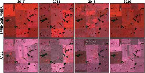
The study area, located in the GNR of Alberta, is within North America’s Prairie Pothole Region (PPR) with an approximate size of 2,645 square kilometers (Figure 1). It is characterized by swamps, marshes, and shallow open water wetlands located within agricultural fields, making this a unique and challenging landscape for wetland mapping. The wetlands in the GNR are typically drained extensively and filled for agriculture, leading to significant wetland loss (Bartzen et al. 2010). Due to their small sizes and high sensitivity to climatic variability, wetlands in the GNR are vulnerable to ecological, hydrological, and anthropogenic changes. In addition, the ponded water areas are highly variable due to changes in wet and dry periods characteristic of spring/summer to fall transitions (Figure 2).

Figure 1. Map of the study area showing (A) the United States and Canada provinces in the Prairie Pothole Region, (B) the natural subregions of Alberta overlayed with the northwestern extent of the Prairie Pothole Region and (C) a summer Sentinel-2 natural composite of the study area for 2020

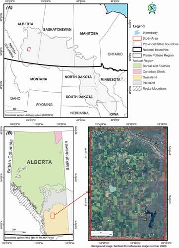
Figure 2. Sentinel-2 multispectral time-series images illustrating the dynamic nature of prairie pothole wetlands in spring/summer (May–August) and fall (September–November) months of 2017, 2018, 2019 and 2020

Alberta has diverse wetland types, which vary in size and surrounding landscapes, presenting various challenges in accurately classifying and delineating these wetlands. Wetlands in the GPNR of southern Alberta are typically small, disconnected prairie pothole marshes and shallow open water habitats surrounded by grasslands, parkland forests, agriculture, and urban areas (Natural Regions Committee 2006; GOA: Aep 2020). The spatial extents of prairie pothole wetlands in the GPNR vary throughout the year and are related to seasonal variations such as snowmelt and precipitation.

2.3. Classification scheme

The Canadian Wetland Classification System (CWCS) defines wetlands as “land saturated with water long enough to promote wetland or aquatic processes as indicated by poorly drained soil, hydrophytic vegetation, and various biological activity adapted to wet environments” (National Wetlands Working Group 1997). The CWCS was developed to support national wetland classification and has since been used throughout peatland-dominated central and northern Alberta’s wetland ecosystems (Alberta Environment and Sustainable Resource Development (ESRD) 2015). The Alberta Wetland Classification System (AWCS) is modified from the CWCS to identify and classify wetlands in Alberta. The AWCS consists of the same five broad classes of wetlands as the CWCS based on their soil, water, and vegetation characteristics: bogs, fens, marshes, shallow open waters, and swamps (Alberta Environment and Sustainable Resource Development (ESRD) 2015). These classes shall provide a framework for analyzing wetland characteristics in the study area using various earth observation data. Available historical information supplied from the Alberta Merged Wetland Inventory (AMWI) database indicates that the prominent wetlands are marsh, swamp, and shallow open water for the study area. Other upland classes considered in this study included cropland, exposed land and barren, forest, grassland, shrubland, and urban and developed. A description of the wetland and upland classes considered in the classification scheme is shown in Table 1.

Table 1. Description of wetland and upland classes considered in the study

Landcover class	Description
Marsh*	Marshes are mineral wetlands that represent the transition zone between shallow open water and basin edge and, in some instances, could exist in isolation. Marshes usually exhibit variable water levels at or above the ground surface at different periods throughout the seasons. Marshes periodically turn dry, exposing the ground surface to oxygen, which results in nutrient enrichment. This condition promotes the growth of diverse emergent and grasslike vegetation (graminoids).
Shallow Open Water (later known as open water)*	Shallow open water bodies are mineral wetlands with a water depth up to a maximum of 2 meters. Open water wetlands receive water through a combination of precipitation, runoff and stream inflow. Deep portions of the open water zone support floating and/or submerged aquatic vegetation contingent on nutrient availability. Open water wetlands are usually permanently flooded and experience water level fluctuations over seasons.
Swamp*	Swamps are considered mineral wetlands (≤40 cm peat depth) and could also exist as peatlands (>40 cm peat depth) in some instances (such as a woody plant cover) comprises more than 25% of the total area. The ground surface is characterized by soils derived from minerals and/or rocks containing little organic material even though sub-surface peat exist in certain situations. The water sources for swamps include a combination of precipitation, runoff, and groundwater. Swamps are transition zones between other wetlands and non-wetlands and typically support high biodiversity.
Uplands**	Uplands comprise croplands, grasslands, urban and developed, forests (broadleaved, coniferous, and mixed), exposed and barren, and shrubland classes. Cultivated cropland or cropland are farmlands planted with annual crop species. The croplands includes small grains (wheat, barley, oats and mixed grains), oilseeds (canola, flax), specialty crops (peas, lentils), and row crops (such as potatoes, sugar beets, corn, vegetables). Fallow describes areas used for producing the crops that do not exhibit visible vegetation due to being cultivated. This cropland information was sourced from a combination of ABMI HFI and the Canada Annual Crop Inventory.

* Sourced from the Government of Alberta (GoA) Alberta Merged Wetland Inventory database

** Sourced from the Alberta Biodiversity Monitoring Institute Human Footprint Inventory database and the Canada Annual Crop Inventory. The shallow open water class cited in the GoA merged wetland inventory was renamed open water for the purpose of this study. This reference is reflected in subsequent text and maps cited or generated in the study.

2.4. Sources of training and testing data used in the study

A significant challenge of wetland mapping in the GNR is the lack of up-to-date and accurate ground data to build the classification models and assess the accuracy of wetland products generated. The ground data used to train the models developed in this study and evaluate their accuracy were open-access government databases. These included the Government of Alberta (GOA)’s AMWI (Government of Alberta) and the Alberta Biodiversity Monitoring Institute (ABMI) Human Footprint Inventory (HFI) database (Alberta Biodiversity Monitoring Institute 2018) and 3 × 7 photo plot data (ABMI 2020).

The AMWI, an amalgamation of 35 wetland inventories, utilized various data sources, years of capture, and classification methods. The AMWI subset for the study area was generated between 2010 and 2011 and done by digitizing orthophotos. This dataset had a spatial accuracy of 0.5 m. In addition, the latest version of the ABMI HFI (HFI_2018), created in 2018, showing disturbances (e.g., agriculture, forestry, energy) across Alberta, was also explored.

The other ABMI-sourced reference data used were 3 × 7 photo plots. This detailed and comprehensive database characterizes vegetation features, wetlands, land use, infrastructure, moisture characterization, land cover, and management status covering approximately 5% of the province. The 3 × 7 photo plot data (last updated in May 2018) served as the baseline reference for extracting the wetland training and testing information to build the classification models and assess their accuracy. It was also used to compare the AMWI database and the optimal wetland classification identified in this study.

In addition to the GOA databases, we used the Canada Annual Crop Inventory (ACI) (Fisette et al. 2013) to classify other upland classes like croplands, grasslands, urban and developed areas, forests (broadleaved, coniferous, and mixed), exposed and barren, and shrubland. For the different years (2017, 2018, and 2019), the ACI was used to extract upland training and testing data. The ACI dataset also guided the delineation of non-wetland classes; a similar approach was demonstrated in Mahdianpari et al. (2020a). Figure 3 shows the spatial distribution of training and testing data (from Canadian data inventories) used for image classification and accuracy assessment in the study.

Figure 3. Training and testing data (from Canadian data inventories) used for image classification and accuracy assessment in the study

The limited availability of training and validation data was a significant limitation in this study. However, like any remote sensing-based work faced with such challenges, other ancillary data, including high-resolution imagery obtained from Google Earth, were consulted to complement the existing publicly available datasets through visual interpretation (Mahdianpari et al. 2020a, 2019). Table 2 describes the training and testing data used in the study for image classification and accuracy assessment

Table 2. Training and testing data used in the study for image classification and accuracy assessment

LCC ID	Landcover class	Training data		Testing data
		Pixel counts	Area (sq km)	Pixel counts	Area (sq km)
1	Marsh*	544,590	54.5	363,398	36.3
2	Open Water*	468,916	46.9	267,761	26.8
3	Swamp*	2340	0.2	1,588	0.2
4	Cropland**	2,981,795	298.2	4,280,635	428.1
5	Grassland**	3,340,260	334.0	901,194	90.1
6	Urban and Developed**	101,323	10.1	119,503	12.0
7	Forest**	18,364	1.8	42,854	4.3
8	Exposed Land and Barren**	193,342	19.3	119,978	12.0
9	Shrubland**	41,948	4.2	41,041	4.1

* Sourced from the Government of Alberta (GoA) Alberta Merged Wetland Inventory database

** Sourced from the Alberta Biodiversity Monitoring Institute Human Footprint Inventory database and the Canada Annual Crop Inventory.

2.5. Remotely sensed data

For this study, we downloaded S1 and S2 satellite images covering the study area from the cloud-based geospatial processing platform GEE (Gorelick et al. 2017). Table 3 summarizes the multi-temporal multi-source optical, radar, and topographic variables evaluated in the study. The S1 and S2 images used were for the spring/summer (15 May to 15 August) and fall (1 September to 15 November) months of 2017, 2018, 2019, and 2020. The S1 data provided within GEE are Ground Range Detected scenes, acquired in dual-polarimetric (VV/VH) Interferometric Wide Swath mode, and pre-processed using the Sentinel-1 Toolbox to Level-1. The total number of S1 images covering the study area for the spring/summer and fall months were 207 and 157, respectively. Details of the number of S1 images covering the study area from 2017 to 2020 are presented in Table 3. The S2 images downloaded from GEE were Top of Atmosphere (TOA) multispectral data for the same time frame as the S1 images. We selected only S2 images with cloud cover <50% in the spring/summer months and <20% in the fall months to maximize the availability of cloud-free scenes. The total number of S2 images for the time series was 766 (604 for the spring/summer and 162 for the fall months).

Table 3. Characteristics of Sentinel-1, Sentinel-2, and LiDAR elevation data explored in the study

Satellite	Input features
	Dates of Sentinel-1 and Sentinel 2 images (dd/mm/yyyy)	Spring/summer: 15/05/2017 – 15/08/2017 15/05/2018 – 15/08/2018 15/05/2019 – 15/08/2019 15/05/2020 – 15/08/2020	Fall: 01/09/2017 – 15/11/2020 01/09/2018 – 15/11/2020 01/09/2019 – 15/11/2020 01/09/2020 – 15/11/2020
Sentinel-1	Channels	VV, VH
	Ratio feature	$\frac{VV}{VH}$
	Number of overlapping images (Sentinel-1)	Spring/summer:	Fall:
		2017 = 51	2017 = 38
		2018 = 49	2018 = 32
		2019 = 54	2019 = 41
		2020 = 53	2020 = 46
Sentinel-2	Selected channels	B2 (Blue), B3 (Green), B4 (Red), B8 (NIR), B11 (SWIR-1), B12 (SWIR-2)
	Spectral indices	$NDVI=\frac{\left(NIR-Red\right)}{\left(NIR+Red\right)}$, $NDWI=\frac{\left(Green-NIR\right)}{\left(Green+NIR\right)}$, $NDSI=\frac{\left(SWIR-NIR\right)}{\left(SWIR+NIR\right)}$
	Number of overlapping images (Sentinel-2)	Spring/summer:	Fall:
		2017 = 55	2017 = 19
		2018 = 207	2018 = 58
		2019 = 164	2019 = 50
		2020 = 178	2020 = 35
	Elevation Data	LiDAR bare earth Digital Elevation Model
	Topographic measure	$TWI=In\left(\frac{A}{tan\left(\beta \right)}\right)$

B: Band, NIR: Near infrared, SWIR: Shortwave infrared, NDVI: Normalized Difference Vegetation Index, NDWI: Normalized Difference Water Index, NDSI: Normalized Difference Soil Index, LiDAR: Light Detection and Ranging, VH: Vertical transmit and horizontal receive polarization, VV: Vertical transmit and vertical receive polarization, and TWI: Topographic Wetness Index (where A is the upslope contributing area, and β is the local slope angle).

The elevation data employed in this study were a high-resolution LiDAR digital elevation model (DEM) processed into 15-m XYZ ASCII grids. The bare earth LIDAR DEM includes the returns within the point cloud from the ground only. The LiDAR15 DEM features had vertical and horizontal accuracies of 30 cm and 50 cm, respectively. For this study, the LiDAR 15 m DEM raster layer was resampled to 10 meters to ensure proper overlap with the Sentinel imagery.

3. Methodology

Figure 4 presents the proposed workflow for mapping wetlands in the study area. This approach utilizes multi-temporal S1 SAR and S2 optical data combined with LiDAR-derived topographic metrics. The methodology includes satellite data pre-processing, selecting the optimal input variables for image classification (feature selection), wetland and upland classification, accuracy assessment, and post-classification refinement.

Figure 4. Proposed workflow for wetland mapping using multi-temporal freely available Sentinel 1 SAR and Sentinel 2 optical data combined with LiDAR-derived topographic metric

3.1. Image pre-processing

3.1.1. Multispectral data

The S2 data (ee.ImageCollection(“COPERNICUS/S2,”) available in GEE) contains 13 unsigned 16 bit integer spectral bands representing TOA reflectance scaled by 10,000. Three additional quality assurance bands, including a bitmask band with cloud mask information (QA60), are present. A customized cloud-masking and compositing script was written in Javascript and implemented in GEE to remove cloud cover and noise presence in GEE’s image composition. As part of the cloud-masking process, the quality flag band (QA60) identifies and masks out flagged cloud and cirrus pixels (Schell and Deering 1973). With Band 1, the outstanding clouds and aerosols were identified and masked out with a threshold of Band 1 ≥ 1500. Using the median image reducer in GEE, the S2 image collection’s median values covering the spring/summer and fall months for 2017 to 2020 were calculated. The spatial resolution of the SWIR band (20 m) was pan-sharpened to 10 m using the NIR band (B8) and the GEE spatial enhancement tool (hsvToRgb – hue, saturation, and value (HSV) color model), as demonstrated by Kau and Lee (2013) and other previous studies (Du et al. 2016; Yang et al. 2017). The S2 median bands were used to calculate the multi-seasonal optical indices (NDVI, NDSI, and NDWI) evaluated in the study. The Supplementary materials present the GEE code for processing and downloading the S2 variables evaluated in this study.

3.1.2. SAR data

The S1 image collection (ee.ImageCollection(“COPERNICUS/S1_GRD”)) available on GEE consists of Level-1 GRD scenes processed to backscatter coefficient (σ°) in decibels (dB). The processing steps using standard algorithms implemented by S1 Toolbox software include: applying orbit files, removing low-intensity noise and invalid data on scene edges, thermal noise removal, radiometric calibration, and orthorectification (Gorelick et al. 2017; ESA 2019). In addition to the GEE standard pre-processing, we applied several additional post-processing steps to the S1 imagery used for the study. These steps included normalizing backscatter coefficients, excluding wind-affected pixels, angular correction and applying the Refined Lee Speckle filter as coded in the SNAP 3.0 S1TBX (Yommy, Liu, and Wu 2015) to the image composition. The speckle filtering significantly reduces granular image noise caused by the interference of transmitted and received microwaves at the radar antenna (Gulácsi and Kovács 2020).

S1 is a phase-preserving dual-polarization SAR system that transmits signals in either horizontal (H) or vertical (V) polarizations. Similarly, S1 receives signals in both H and V polarizations. Thus, the S1 C-band SAR instrument supports operation in single polarization (HH or VV) and dual-polarization (HH+HV or VV+VH), implemented through one transmit chain (switchable to H or V) and two parallel receive chains for H and V polarization (ESA 2021).

For the study area, the available dual-polarization dataset was the VV-VH channels. Therefore, we used the mean dual-polarization bands (VV and VH) acquired same time as the S2 data to calculate the dual-polarization ratio (VV/VH). The Supplementary materials present the GEE code for processing and downloading the dual-polarization data evaluated in this study.

3.1.3. Topographic data

The LiDAR data were used to calculate the topographic index TWI, which describes the ground’s potential wetness based on topography (Boehner et al. 2001; Conrad et al. 2015; Sörensen, Zinko, and Seibert 2006). The TWI serves as a proxy for the relative soil moisture (Raduła, Szymura, and Szymura 2018) and spatial distribution of wetland processes (Moore, RB Grayson, and Ladson 1991). The TWI is a widespread index in hydrological analysis that describes an area’s tendency to accumulate water (Boehner et al. 2001; Mattivi et al. 2019). Studies have demonstrated the value of LiDAR-based topographic metrics such as TWI in improving the accuracy and automation of wetland mapping (Higginbottom et al. 2018; Lang et al. 2013). The TWI index is a function of both the slope and the upstream contributing area per unit width orthogonal to the flow direction. In addition, it is correlated with soil attributes such as horizon depth, silt percentage, organic matter content, and phosphorus (Moore, Lewis, and Gallant 1993). Therefore, the areas prone to water accumulation (large contributing drainage areas) and characterized by low slope angle will be linked to high TWI values. On the other hand, well-drained dry regions (steep slopes) are associated with low TWI values. However, which particular TWI values indicate wet soils vary depending on landscape, climate, and scale (Ågren et al. 2014). The TWI was computed using the System for Automated Geoscientific Analyses open-source software (Saga 2013). Table 3 presents the formula for calculating TWI.

3.2. Feature selection for classification

There exist diverse approaches to determining relevant or important band(s) that contribute to informed land-use/landcover class decisions. However, studies show no unique approach to establishing an individual separability measure to select valuable band input(s) to distinguish various landcover classes (Hird et al. 2017). This study explores the combined use of band correlation and variable importance using the random forest (RF) algorithm. Using the R open-source statistical software (R Core Team 2020), we checked for band correlation between all the input variables evaluated in the study.

3.3. Machine learning classifier algorithms

For this study, RF, SVM, and CART ML classifier algorithms (present in GEE) were adopted. This cloud-based supervised classification approach collects the necessary information to train the classifiers from training points (Chen and Stow 2002). The GEE JavaScript function requires a set of inputs: the area of interest defining the study area, feature class collection of features containing labeled training data with codes corresponding to the land-use/landcover (LULC) classes, and a dataset composition of selected input variables for classification. The training labels were points generated in a stratified random manner within the training polygon layers used in the study. The training polygons were rasterized in ArcGIS Desktop (version 10.8) software (ESRI 2020) and uploaded to GEE as an asset.

The RF classifier has gained immense attention in landcover mapping using satellite imagery (Amani et al. 2017a; Belgiu and Drăguţ 2016; Immitzer, Atzberger, and Koukal 2012). This non-parametric ensemble learning algorithm (Breiman 2001) outperforms traditional decision trees (Amani et al. 2017b; Immitzer, Atzberger, and Koukal 2012). The RF algorithm constructs multiple de-correlated random decision trees that are bootstrapped and aggregated to classify a dataset using the mode. While implementing the RF classifier, users need to specify the number of decision trees and randomly selected variables for splitting the trees (Onojeghuo and Onojeghuo 2017). After several trials and fine-tuning, the RF algorithm on GEE had 250 decision trees and modeled using the stratified random sample points. The GEE JAVA line code to perform RF classification (ee.Classifier.smileRandomForest()) creates an empty RF classifier in the GEE environment. The RF algorithm is well known for handling high-dimensional datasets such as hyperspectral imagery, making it a suitable approach for classifying complex landscapes (Ghimire et al. 2012).

Studies have demonstrated the value of using SVM classifier to perform landcover classification with multispectral images (Pal and Mather 2005; Sui, He, and Fu 2019). Dixon and Candade (2008) indicated that SVM performed better than traditional classifiers and required less training time. The SVM classifier is a non-parametric distribution-free supervised ML classifier (Vapnik and Vapnik 1998). SVM has been successfully used to classify medium and very high-resolution satellite imagery accurately (Sui, Bin, and Tianjiao 2019). Previous studies have reviewed and documented SVM use in remote sensing applications (Mountrakis, Jungho Im, and Ogole 2011; Huang, L. S. Davis, and Townshend 2002; Pal 2005). SVM models in GEE support different kernels, such as linear and radial basis functions (RBF). The study by Mountrakis, Jungho, and Ogole (2011) showed that the RBF kernel parameter performed best compared to other kernels. The RBF kernel nonlinearly maps samples into a higher-dimensional space, so it, unlike the linear kernel, can handle the case when the relation between class labels and attributes is nonlinear (Hsu, Chang, and Lin 2003). Both classifiers (RF and SVM) have higher accuracy than traditionally based classifiers while using fewer training data (Onojeghuo and Onojeghuo 2017).

In addition to the RF and SVM ML classifiers, we evaluated the use of CART for wetland classification. CART involves identifying and constructing a binary decision tree using a sample of training data for which the correct classification is known. The CART decision tree is a binary recursive partitioning procedure capable of processing continuous and nominal attributes as targets and predictors (Steinberg and Colla 2009). The numbers of entities in the two sub-groups defined at each binary split, which correspond to the two branches emerging from each intermediate node, become successively smaller so that a reasonably large training sample is required if good results are to be obtained (McLachlan 1992). The ee.Classifier.smileCart()line code in GEE was used to classify the image composite. The code creates an empty CART classifier in the GEE environment. The advantage of decision tree algorithms in image classification over traditional classifiers like MLC is their ability to deal with complicated dataset distribution. When handling remote sensing image features with different statistical distributions and scales, decision tree classifiers obtain the best results.

Using the RF classifier as the basis for selecting the optimal multi-temporal composite, we performed a pixel-by-pixel comparison with CART and SVM wetland classified maps generated in the study.

3.4. Accuracy assessment

For this study, two stages of accuracy assessment were performed. The first considered all the fused datasets presented in Table 4, while the second compared the AMWI and the optimal wetland inventory from this study. The details of both approaches’ accuracy results are shown in Sections 4.2, 4.3, and 4.4, respectively. For this study, we utilized visual inspection, compared error matrices, and calculated Kappa statistics for all classification outcomes. The visual inspection included a comparison with existing high-resolution orthoimages and satellite imagery. For statistical evaluation, error matrices for all classified outputs were constructed and used to calculate the User’s Accuracy (UA), Producer’s Accuracy (PA), Overall Accuracy (OA), and F-score of all landcover classes (Congalton and Green 2019; Powers 2011). Equations 1(1) $UA=\frac{X_{ij}}{X_j}\times 100\mathrm{\%}$(1) –4(4) $\mathrm{F}-\mathrm{s}\mathrm{c}\mathrm{o}\mathrm{r}\mathrm{e}=2\times \frac{UA\times PA}{UA\times PA}$(4) show how to calculate the UA, PA, OA, and F-scores.

(1) $UA=\frac{X_{ij}}{X_j}\times 100\mathrm{\%}$(1)

(2) $PA=\frac{X_{ij}}{X_i}\times 100\mathrm{\%}$(2)

(3) $OA=\frac{S_d}{n}\times 100\mathrm{\%}$(3)

(4) $\mathrm{F}-\mathrm{s}\mathrm{c}\mathrm{o}\mathrm{r}\mathrm{e}=2\times \frac{UA\times PA}{UA\times PA}$(4)

Table 4. Fused datasets used for experiments utilizing multi-seasonal (spring/summer & fall) Sentinel-1 radar and Sentinel-2 multispectral data and LiDAR-derived topographic variables (where B8 = near-infrared band, B11 = shortwave infrared band, VH = vertical and horizontal dual-polarization channel, TWI = topographic wetness index)

Experiment #	Dataset #	Fused data	Classifier	Number of bands	Year
1	1	(B8 + B11 + VH) + TWI	RF	7	2017
2	2	(B8 + B11 + VH) + TWI	RF	7	2018
3	3	(B8 + B11 + VH) + TWI	RF	7	2019
4	4	(B8 + B11 + VH) + TWI	RF	7	2020
5	5	Datasets 1 + 2 + 3 + 4	RF	25	2017-2020
6	6	Datasets 1 + 2 + 3 + 4	CART	25	2017-2020
7	7	Datasets 1 + 2 + 3 + 4	SVM	25	2017-2020

where X_ij = observation in row i column j, Xi = marginal total of row i, X_j = marginal total of row j, S_d is the total number of correctly classified pixels, and n = total number of validation pixels.

We used McNemar’s test to analyze statistically significant differences for all classified maps generated in the study (Agresti 1996; Bradley 1968). McNemar’s test is a non-parametric test applied to confusion matrics with a 2 × 2 dimension. Equation 5(5) $z=\frac{\left(f_{12}-f_{21}\right)}{\sqrt{\left(f_{12}-f_{21}\right)}}$(5) presents the standardized normal static on which the test is based:

(5) $z=\frac{\left(f_{12}-f_{21}\right)}{\sqrt{\left(f_{12}-f_{21}\right)}}$(5)

where f₁₂ and f₂₁ are the off-diagonal entries in the matrix. The difference in accuracy between a pair of classifications is considered significant at a confidence level of 95% if the calculated z score is more than 1.96 (positive or negative). Also, if the z score is more than 2.58, it has a 99% confidence level. The method for calculating and presenting the z scores was similar to that shown in Onojeghuo and Onojeghuo (2017).

3.5. Post-classification refinement of optimal wetland inventory

This stage of the study aimed to refine the optimal wetland inventory by removing erroneously classified pixels. The first step was a visual inspection of the optimal wetland image using a combination of multi-date high-resolution imagery (such as the Esri high-resolution ortho-imagery (dated January 2018) and the S2 multispectral image). During the visual inspection, misclassified wetland pixels were identified and reclassed to upland classes. To further refine the wetland classification, a “median filter” was applied. The median filter ranks the input cell values in the filter window in numerical order and assigns the median value (middle value in the rank order) as the output. Because the output value is not affected by the actual value of outlier cells within the filter window, the median filter is particularly good at removing isolated random noise (TNTMips 2014). Next, the median filtered wetland classification was converted to a polygon feature layer and smoothened using the “polynomial approximation with exponential kernel smoothing algorithm” available in ArcGIS. We selected a tolerance of 50 m for the smoothing process. The wetland polygon layer was further filtered to exclude any areas less than 0.04 hectares. This area complies with the minimum mapping unit stated in the Alberta Wetland Mapping Standards report (GOA: Aep 2020) for wetland mapping in Alberta’s prairie and parkland wetland regions.

3.6. Comparison of optimal wetland map with Alberta merged wetland inventory reference database

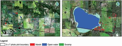
For wetland mapping projects, it is standard practice to compare generated wetland maps with fine-resolution satellite images or orthophotographs to validate the results obtained in the absence of coincident ground truth reference data (Huang et al. 2018). This study’s primary challenge was the absence of concurrent field data and finer resolution satellite or airborne imagery in the public domain. We utilized the AMWI (Government of Alberta) and ABMI 3 × 7 photo plot data (ABMI 2020) in the absence of up-to-date fine-resolution reference maps or ground data. Using the available wetland information provided in the 3 × 7 photo plot data, we reclassified the ABMI 3 × 7 reference layer to reflect wetland classes according to the AWCS classification scheme described in Section 2.3 of this paper (see Figure 5). With the 3 × 7 photo plot data, a stratified sampling approach to extracting ground reference validation points needed for accuracy assessment was performed using ArcGIS software (ESRI 2020). We collected 386 reference points representing the three wetland classes (marsh: 150, open water: 150, and swamp: 86) for accuracy assessment. Figure 5 shows examples of the reclassified ABMI 3 × 7 photo plot data reference layer used for wetland comparison.

Figure 5. Examples of the reclassified Alberta Biodiversity monitoring institute 3 × 7 photo plot data reference layer used for wetland comparison

4. Results

4.1. Feature selection and data exploration results

For this study, the input data evaluated for each time-stamp (spring/summer and fall, 2017–2020) comprised of the following: B8 (NIR) and B11 (SWIR), NDVI, NDSI, NDWI, VH, VV/VH ratio, and TWI. The input band correlation tests were performed to understand the correlation between input bands considered in the study. This information, combined with the RF variable importance test, informed the final selected input variables used for wetland and upland classification. The supplementary material presents the RF variable importance results (Figure S.1 – S.4), the box plots of each land cover class (Figure S.5), and the band correlation results of the evaluated input variables considered in the study for 2017, 2018, 2019, and 2020 (Figure S.6 – S.9). The RF variable importance test showed the VH channel performed better than the other two evaluated (VV and VV/VH) for the assessed years (2017, 2018, 2019, and 2020). The results indicate that for all the wetland and upland classes, the VH channels of both seasons for all the years performed better than the other two S1 variables. Based on these results, the input variables with the least correlation and considered most important for the RF classification (having reasonable mean pixel distribution per class) were B8 (NIR), B11 (SWIR), VH, and TWI. These selected bands formed the basis for generating the multi-seasonal image composites evaluated in the study (Figure 4, Table 4). Figure 4 presents the input layers assessed in the study. Table 4 summarizes the input datasets used for the image classification experiments. The first five experiments were designed to evaluate the performance of combining selected multi-temporal S1 and S2 and LiDAR-derived TWI (B8+ B11+ VH+TWI) for different periods (2017 to 2020). Experiment 1 used the features chosen for 2017, while Experiments 2, 3, and 4 were for 2018, 2019, and 2020. Experiment 5 combined all four time periods (2017, 2018, 2019, and 2020). Experiments 1–5 were conducted using the RF classifier algorithm using the same number of trees (k) as 250.

4.2. Accuracy assessment of RF experiments using multi-temporal Sentinel SAR and optical data fused with LiDAR topographic metric

This phase of the study aimed to evaluate the performance of multi-temporal S1 and S2 data fused with LiDAR-derived TWI for wetland mapping. First, we conducted the pre-classification experiments with the RF classifier algorithm. Then, the best performing datasets were selected and used to analyze further the SVM and CART classifiers based on the accuracy assessment results.

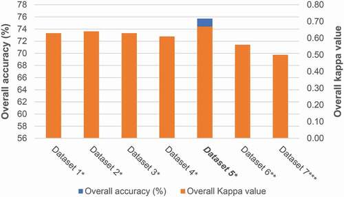
Figure 6 presents the classification accuracy results. The results showed the RF classifier’s performance on the multi-temporal S1 and S2 images fused with the LiDAR-derived TWI for the four-time periods (2017–2020) had overall accuracies ranging from 71 to 76% (i.e., Dataset 1–5). The best performing RF classified dataset evaluated in the study was Dataset 5, with an overall accuracy of 76%, which significantly outperformed Datasets 1–4 at a 99% confidence level (see Figure 6, Table 5). The kappa values also showed corresponding improvements as the overall accuracies. McNemar’s test results showed no significant difference between Experiments 1 and 3 (Table 5). The best combination of F-score values of the RF-classifier experiments was for Dataset 5 (a fusion of the four years S1 and S2 multi-temporal images combined with the LiDAR-derived TWI) – 0.61 (marsh), 0.82 (open water), 0.75 (swamp), and 0.8 (uplands) (see Table 6). Table S.10 in the Supplementary document presents the error matrices of the classifications performed in the study.

Table 5. McNemar’s test results of classifications performed in the study

Dataset/Classifier	Tests	z-score
Dataset 1–5 (RF)	1 vs 2	4.58**
	1 vs 3	1.83
	1 vs 4	6.63**
	1 vs 5	9.06**
	2 vs 3	4.93**
	2 vs 4	8.06**
	2 vs 5	7.81**
	3 vs 4	6.38**
	3 vs 5	9.24**
	4 vs 5	11.22**
Dataset 5–7 (optimal RF classification, SVM and CART classification)	RF vs SVM	17.81**
	RF vs CART	14.53**
	SVM vs CART	10.31**
Optimal RF classification and AMWI wetland map	AMWI vs RF	1.63

Considered significant at a confidence levels of 95% (z ≥ 1.96 (positive or negative)) and 99% (if z ≥ 2.58). Where ** denotes 99% significant.

Table 6. Per-class accuracy results of multi-temporal Sentinel SAR and optical data fused with LiDAR topographic index evaluated in the study (best results in bold and italics)

Random Forest classification experiments (Experiments 1, 2, 3, 4, and 5)
Class	PA (%)	UA (%)	F-score
Dataset 1 – RF
Marsh	39.5	68.7	0.50
Open water	83.1	89.5	0.86
Swamp	73.5	79.1	0.76
Upland	94.1	60.6	0.74
Dataset 2 – RF
Marsh	44.3	68.7	0.54
Open water	84.9	83.6	0.84
Swamp	67.1	80.7	0.73
Upland	95.7	65.0	0.77
Dataset 3 – RF
Marsh	43.8	66.6	0.53
Open water	84.2	85.9	0.85
Swamp	66.3	78.7	0.72
Upland	93.9	63.1	0.75
Dataset 4 – RF
Marsh	39.2	62.4	0.48
Open water	83.4	85.5	0.84
Swamp	65.0	74.8	0.70
Upland	94.3	62.8	0.75
Dataset 5 – RF
Marsh	50.0	78.9	0.61
Open water	86.7	78.4	0.82
Swamp	67.5	85.5	0.75
Upland	97.0	68.0	0.80
CART and SVM classification experiments (Datasets 6 and 7)
Dataset 6 – CART
Marsh	38.4	59.5	0.47
Open water	83.5	83.2	0.83
Swamp	50.4	79.2	0.62
Upland	93.8	57.1	0.71
Dataset 7 – SVM
Marsh	38.4	79.5	0.58
Open water	83.5	83.2	0.75
Swamp	50.4	79.2	0.56
Upland	93.8	57.1	0.64

Figure 6. Graph showing the classification accuracy results in the study. The best performing dataset (Dataset 5) generated using the RF classifier (* denotes RF, ** CART, and *** SVM classified datasets)

4.3. Optimal multi-date SAR, optical, and TWI data results: RF, SVM, CART

Using the RF classifier, the best accuracies were achieved for Experiment 5 (i.e., Dataset 5), combining all selected S1, S2, and TWI input variables for 2017, 2018, 2019, and 2020. The SVM and CART classifiers were further applied to Dataset 5 to evaluate their performance. After a series of trials for the SVM algorithm, the RBF kernel was used for classification in the GEE geospatial platform. The classification experiments showed that Experiment 5 (RF) had the best overall accuracy of 75.6%, followed by Experiment 6 (CART) with 67.4%, and Experiment 6 (SVM) with 63.2% (see Figure 6). Results of McNemar’s test showed significant differences among the three classifiers (Table 5).

The per-class accuracy results (shown in Table 6) combined the producer’s and user’s accuracy results to calculate the F-score measure. Experiment 5 (RF) had the best combination of wetland and upland F-score values. The highest F-score for marsh was 0.61 for Experiment 5 (RF), followed by Experiment 7 (SVM) with 0.58 and Experiment 6 (CART) with 0.47. For open water, the F-score values in order of the highest to the lowest were 0.83 (Experiment 6), 0.82 (Experiment 5), and 0.75 (Experiment 7). The best performing classifier for swamp identification was RF (0.75, Experiment 5), followed by the CART classifier (0.62, Experiment 6) and SVM classifier (0.56, Experiment 7) (see Table 6). Similar to the swamp wetland class, the best F-score value for the upland was 0.8 (RF, Experiment 5), followed by 0.71 (Experiment 6, CART) and 0.64 (Experiment 7, SVM).

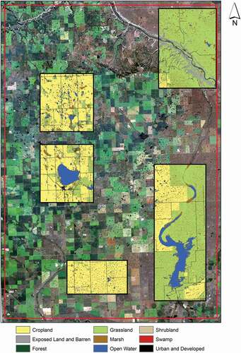
The RF classifier performed best to classify marsh, swamp, and upland classes, while CART performed best to identify open water. The diversity in the performance of all three classifiers was related to discrepancies in their concepts. Figure 7 presents the optimal RF derived wetland inventory generated using a multi-seasonal image composite comprised of S2 optical (B8 and B11), S1 radar (VH) fused with LiDAR-derived TWI over the spring/summer and fall months for 2017 to 2020.

Figure 7. Optimal wetland classification generated using multi-temporal Sentinel-2 multispectral and Sentinel-1A radar imagery fused with LiDAR-derived Topographic Wetness Index

4.4. Comparison of optimal RF wetland map and Alberta Merged Wetland Inventory

This component of the study involved comparing the optimal RF wetland map to the AMWI dataset. The wetland types in the AMWI dataset for the study area included marsh, open water, and swamps. The prominent wetland class for both datasets was the marsh. The AMWI wetland product equated to 66.9% of the study area, while the optimal wetland inventory (Dataset 5) was 54.8% (Table 7). Table 7 provides the spatial extent and statistics of the AMWI dataset and this study’s optimal wetland inventory.

Table 7. Summary statistics of the Alberta merged wetland inventory dataset and optimal wetland map generated in this study

Wetland type	Count	Min (ha)	Max (ha)	Mean (ha)	Median (ha)	Sum (ha)	Area percentage
AMWI wetland
Marsh	32,958	0.000025	127.89	0.44	0.21	14,591	66.9%
Open water	3033	0.000025	2,318.11	2.37	0.19	7,177	32.9%
Swamp	153	0.000025	4.57	0.36	0.21	55	0.3%
Total (polygons)	36,144	0.000075	2,450.57	3.17	0.21	21,823	100.0%
Dataset 5 (Experiment 5)
Marsh	31,014	0.04	247.74	0.44	0.14	13,700	54.8%
Open water	1,624	0.04	2,598.85	5.14	0.91	8,355	33.4%
Swamp	9,517	0.04	20.85	0.31	0.12	2,935	11.7%
Total (polygons)	42,155	0.12	2,867.44	5.90	0.14	24,990	100.0%

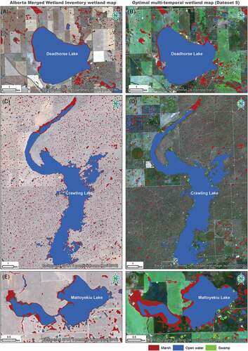
As indicated in Section 2.4, we used the 3 × 7 photo plot data to generate ground reference points to assess the reference AMWI wetland map and the RF-classified optimal multi-date dataset (i.e., Dataset 5, Experiment 5) established in this study. For this purpose, a total of 386 points were randomly extracted for accuracy assessment purposes. The accuracy assessment results showed that the optimal wetland map (Dataset 5) had an overall accuracy of 67.4%, while the AMWI wetland map was 65.3% (Table 8). Table 8 summarizes the accuracy results of both wetland maps compared. In addition, the McNemar’s test showed no significant difference between the OA of the AMWI and Dataset 5 wetland maps (Table 5). Figure 8 presents an example of wetlands identified in the AMWI database and the optimal multi-temporal wetland classification. Also, Figure 9 compares the optimal wetland inventory identified in this study with medium resolution Sentinel-2 natural composite images.

Table 8. Classification accuracy results of AMWI and Dataset 5 wetland maps

Class Name	Reference totals	Classified totals	Number correct	Producers Accuracy (%)	Users Accuracy (%)
AMWI wetland map
Unclassified	1	54	0	-	-
Marsh	150	172	112	74.7	65.1
Open water	150	160	140	93.3	87.5
Swamp	86	0	0	-	-
Total	386	386	252
Overall Accuracy – 65.3% & Overall kappa value – 0.48
Dataset 5-RF wetland map
Unclassified	0	35	0	-	-
Marsh	150	171	104	69.3	60.8
Open water	149	159	140	94.0	88.1
Swamp	87	21	16	18.4	76.2
Total	386	386	260
Overall Accuracy – 67.4% & Overall kappa value – 0.50

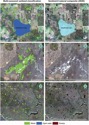
Figure 8. Comparison of AMWI and optimal multi-temporal wetland products of selected sites in the study area – Deadhorse Lake (A and B), Crawling Lake (C and D), and Mattoyekiu Lake (E and F)

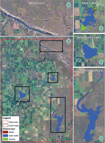
Figure 9. Examples of selected areas in Figure 7 showing a visual comparison of the optimal wetland inventory (a, c, and e) and medium resolution Sentinel-2 natural composite image (b, d, and f)

5. Discussion

5.1. Feature selection for wetland classification

We performed a multi-seasonal variable importance test to establish the relevant input bands for the spring/summer and fall months of 2017, 2018, 2019, and 2020. The first 10 variables ranked as important by the RF model were selected as inputs for subsequent analysis for each year. Compared with other ML algorithms (like an artificial neural network), the RF models are not sensitive to high predictor collinearity. This is because RF algorithms use a subset of the predictors (i.e., input bands) to construct each decision tree (Kamusoko 2019). Each year’s multi-seasonal variable importance test was performed to rank the input variables as most important in the RF model classification. The reoccurring optimal features (variables) for the period examined were used to determine the best multi-seasonal composite. This approach accounted for seasonality effects in the analysis, addressing a vital objective of this study.

Selecting the most optimal features for use in the classification is critical for accurate depictions of the wetland and upland classes. Previous studies have identified the optical, SAR, and topographic features listed in Table 3 to have the highest potential to discriminate various wetland species considered in this study (Amani et al. 2019a, 2018). Ozesmi and Bauer (2002) identified the NIR band as very important in delineating vegetation from open water bodies, which are essential inputs for wetland classification. Also, the SWIR channels provided in the S2 optical imagery can detect moisture levels in vegetation and soil, which are typically wet. The visible bands, particularly the red channel, have been demonstrated to be of value for detecting wetland classes, as shown in previous studies (Amani et al. 2018; Große-Stoltenberg et al. 2016). The SAR features, VV polarization, and VH polarizations help detect flooded wetlands and discriminate herbaceous and woody wetlands (such as marshes and swamps) (Henderson and Lewis 2008; Corcoran, Joseph F Knight, and Gallant. 2013). The S1 dual-polarization ratios (VV/VH) discriminates between herbaceous and woody wetlands (Bourgeau-Chavez et al. 2009; Mahdianpari et al. 2019). The use of elevation data-derived measures, such as TWI, is an essential consideration for wetland identification (Higginbottom et al. 2018; Sörensen, Zinko, and Seibert 2006).

5.2. High-resolution wetland mapping in the GNR

This study developed a workflow that utilizes freely available high-resolution and temporally dense S1 (SAR) and S2 (optical) data fused with LiDAR-derived TWI to generate a 10-m spatial resolution wetland inventory of a study area in the GNR. The supervised pixel-based RF ML classifier and Sentinel satellite open-access data available on GEE geospatial platform provided a powerful and user-friendly medium for wetland classification. The open-access and free availability of the Sentinel satellite images have provided a high temporal frequency of good-quality observation, a valuable information source complemented by LiDAR TWI for wetland mapping in the GNR. The GEE geospatial platform allows us to access the rich repository of Sentinel satellite data, upload external datasets (such as the LiDAR index and training data), and perform image analysis with a parallelized approach (Gorelick et al. 2017). This study utilized seasonal radar and optical data from the Sentinel satellite images acquired in the spring/summer (May–August) and fall (September–November) months of 2017 to 2020 combined with LiDAR TWI data. As indicated in Section 4.3, the RF classifier performed best overall compared to the CART and SVM classifiers algorithms and a more robust approach for wetland mapping in the study. Studies have demonstrated the ability of RF to handle effects of high data dimensionality and generating more accurate classification in comparison to other classifiers such as SVM, maximum likelihood and single decision trees (Gislason, Jon Atli Benediktsson, and Sveinsson 2006; Belgiu and Lucian 2016; Rodriguez-Galiano et al. 2012; Pelletier et al. 2016).

Comparing our optimal wetland map and the available government database (AMWI) showed some differences among both datasets (Figure 8, Table 7). Compared to the AMWI wetland map, our generated wetland map had 1,178 hectares more open water and 2,880 hectares more swamp. The total marsh extent for our wetland map was 891 hectares less than the AMWI wetland product. The differences in the spatial size of the compared wetland maps (i.e., AMWI versus Dataset 5) were due to the different mapping techniques used for both products and dates generated. The method employed in this study differs from the manual digitization of the orthophoto technique used to create the AMWI dataset. In addition to the manual digitization approach, the workflow proposed in this study utilizes a consistent data source (such as Sentinel satellite data) that depicts the recent distribution of wetland habitats in the study area. The AMWI database (Government of Alberta), which provides wetland distribution from 1998 to 2017, needs updating to ensure that current and accurate baseline information can aid effective decision-making and proper policy implementation. An accurate and up-to-date wetland monitoring system is vital for appropriate management, conservation, and wetlands protection. With more high-resolution training data overlapping the Sentinel data’s time coverage, the accuracy of wetland maps in Alberta’s GNR will improve significantly.

5.3. Implication and future development of wetland mapping in GNR

The workflow developed in this project presents vital information necessary for understanding the spatial distribution of wetland habitats across the seasonally dynamic GNR of Alberta. The pixel-based RF classified dataset comprised of multi-temporal (2017–2020) Sentinel SAR (VH) and optical (B8 and B11) bands fused with LiDAR-derived TWI showed to map wetlands in the study area accurately. In the GNR, wetlands are relatively small and have shallow depths susceptible to climatic variability resulting in temporally and spatially dynamic habitats. These characteristics make mapping these wetlands a challenging task. In theory, the fusion of multi-temporal optical, radar, and topographic information should be sufficient to provide the information required for wetland mapping. This study hypothesizes that seasonal SAR and optical imagery will capture temporal variations of wetlands in the spring/summer and fall months of 2017, 2018, 2019, and 2020, while topographic variability offered with the LiDAR-derived TWI shall result in the accurate delineation of the wetlands as demonstrated in Hird et al. (2017). We have shown the value of seasonal multi-temporal SAR and multispectral inputs combined with LiDAR-derived topographic index (TWI) for wetland mapping in the study area. Based on this study’s results, other potential application areas include: (1) tracking the dynamic nature of wetland habitats in the region at fine-resolution 10-m scales and (2) upscaling the approach to include the entire PGNR and similar PPR provinces across Canada. A crucial requirement for this workflow to be up-scaled is to access publicly available and accurate ground truth data across the region for remote sensing classification.

By harnessing the rich repository of Sentinel satellite imagery available on GEE, we can access high-resolution and temporally dense SAR and optical data needed for wetland classification. LiDAR data usage usually has some financial implications associated with its use. In large-scale upscaling of this approach, such cost could be a constraint for operational roll-outs. An alternative option, preferably freely available datasets or cheaper options, is suggested to mitigate this effect. As an alternative to LiDAR elevation data, we can adopt open-access elevation data such as the ALOS World 3D 30-meter digital surface model dataset (Tadono et al. 2014) available on GEE. These open-sourced elevation datasets could be used to calculate the topographic index (such as TWI) that significantly improves the study’s classification accuracy of wetlands. The high-resolution JAXA-ALOS AW3D 5-m digital surface model data (AW3D 2020) is a better substitute for LiDAR elevation data than the ALOS World 3D 30-m data and could be aggregated to 10-m resolution for use with Sentinel data. However, this world elevation product is not freely available.

Active remote sensing techniques such as SAR and LiDAR utilize the differences in topographic structure, vegetation structure, and surface wetness (such as TWI) to map wetlands. Millard et al. (2020) explored the value of full growing time-series Sentinel-1 coherent time-series data for peatland mapping. These authors hypothesized that specific SAR characteristics (like interferometric coherence, amplitude, and differences in amplitude of the time-series datasets) might be able to capture subtle changes in phenology and hydrology, which in turn differentiate classes throughout a growing season. Using seasonal time-series imagery to classify wetland-type classes shows immense potential for operational use and possible upscaling where needed. The limitation of this approach for our study is the non-availability of S1 data on GEE with the original slant-range data. The current S1 SAR data available on GEE includes the polarization bands (single polarization VV and HH, dual-polarization VV+VH or HH+HV). Each scene has an additional “angle” band that contains the approximate viewing incidence angle in degrees at every point.

The complementary characteristics of optical, radar, and elevation data have been shown to enhance the detection of forested and non-forested wetlands (Bwangoy et al. 2010). By adopting a multi-sensor approach that includes the fusion of optical, SAR, and topographic indices, we can now overcome the difficulties imposed by cloud cover and improve the final accuracies of wetland map products. The Supplementary materials present the GEE experimental App that shows the optimal wetland inventory generated in this study.

6. Conclusion

Previous efforts to map wetlands in the GNR generally depended on visual interpretation, supervised and unsupervised classification methods, and the use of single-date or multi-date image mosaics. For this study, we have developed a workflow that utilizes freely available high-resolution and temporally dense S1 (SAR) and S2 (optical) data fused with LiDAR-derived TWI for wetland mapping (10-m spatial resolution). The supervised pixel-based RF ML classifier and Sentinel open-access satellite data on the GEE geospatial platform provided a powerful and user-friendly framework for wetland classification. This study utilized seasonal radar and optical data from the Sentinel satellite images acquired in the spring/summer (May–August) and fall (September–November) months of 2017 to 2020. The classification experiments showed that Experiment 5 (RF) had the best overall accuracy of 75.6%, followed by Experiment 6 (CART) with 67.4%, and Experiment 6 (SVM) with 63.2%.

Most wetland inventories are static datasets generated from one-time airborne or satellite imagery, which typically do not reflect seasonal or annual wetland changes. The increasing availability of cloud-based Sentinel-1A radar and Sentinel-2A multispectral l imagery from ESA combined with LiDAR-derived TWI holds immense potential for mapping the temporal variability of wetlands. This study’s next steps shall include upscaling this developed approach to a regional scale, utilizing the multi-date classification as inputs for a wetland inventory and monitoring system. We will also investigate the use of deep learning classifiers on these input data for wetland mapping. Overall, this study’s results demonstrate GEE’s potential with its rich repository of freely available Sentinel satellite data combined with topographic information to map wetlands in the GNR of southern Alberta. Our GEE-based workflow holds great potential to efficiently and effectively map wetlands in the GNR while improving decision-support and habitat management applications at regional scales when up-scaled.

Highlight

• High-resolution and temporally dense Sentinel-1 (S1) radar and Sentinel-2 (S2) optical data fused with Light Detection and Ranging (LiDAR)-derived topographic metric (Topographic Wetness Index) shows potential for wetland mapping.

• The pixel-based Random Forest (RF) classified dataset comprised of multi-temporal (2017–2020) S1 SAR (VH) and S2 optical (B8 and B11) bands fused with LiDAR-derived TWI had the highest overall accuracy (75.6%).

• The Random Forest classified wetland product significantly outperformed classification and regression tree (CART) and support vector machine (SVM) classifications, which had overall accuracies of 67.4% and 63.2%, respectively.

Disclosure statement

No potential conflict of interest was reported by the author(s).

Supplementary material

Supplemental data for this article can be accessed here.

Data and Codes Availability Statement

The authors confirm that the data supporting the findings of this study are available within the article and its supplementary materials.

Additional information

Funding

This research was funded by the National Research Council (NRC) Industrial Research Assistance Program (Project number 932455) and Solstice Canada Corp. o/a Solstice Environmental Management.

References

- ABMI. “3 X 7 Photoplot Land Cover Data.” Accessed December 27 2020. https://abmi.ca/home/data-analytics/da-top/da-product-overview/Advanced-Landcover-Prediction-and-Habitat-Assessment–ALPHA–Products/Photoplot-Land-Cover-Data-Training-and-Validation.html.
- Adam, E., O. Mutanga, and D. Rugege. 2010. “Multispectral and Hyperspectral Remote Sensing for Identification and Mapping of Wetland Vegetation: A Review.” Wetlands Ecology and Management 18 (3): 281–296. doi:https://doi.org/10.1007/s11273-009-9169-z.
- Aep, G. O. A. 2020. Alberta Wetland Mapping Standards and Guidelines: Mapping Wetlands at an Inventory Scale V1.0. Edmonton, Canada: Government of Alberta - Alberta Environment and Parks.
- Ågren, A. M., W. Lidberg, M. Strömgren, J. Ogilvie, and P. A. Arp. 2014. “Evaluating Digital Terrain Indices for Soil Wetness Mapping–a Swedish Case Study.” Hydrology and Earth System Sciences 18 (9): 3623–3634. doi:https://doi.org/10.5194/hess-18-3623-2014.
- Agresti, A. 1996. An Introduction to Categorical Data Analysis. New York, N.Y.: Wiley.
- Alberta Biodiversity Monitoring Institute. 2018. Human Footprint Inventory 2018 (Version 1). Alberta, Canada: Geospatial Center, Alberta Biodiversity and Monitoring Insitute.
- Alberta Environment and Sustainable Resource Development (ESRD). 2015. “Alberta Wetland Classification System. Water Policy Branch, Policy and Planning Division, Edmonton, AB.”
- Amani, M., B. Brisco, S. Majid Afshar, M. Mirmazloumi, S. Mahdavi, S. M. J. Mirzadeh, W. Huang, and J. Granger. 2019a. “A Generalized Supervised Classification Scheme to Produce Provincial Wetland Inventory Maps: An Application of Google Earth Engine for Big Geo Data Processing.” Big Earth Data 3 (4): 378–394. doi:https://doi.org/10.1080/20964471.2019.1690404.
- Amani, M., B. Salehi, S. Mahdavi, and B. Brisco. 2018. “Spectral Analysis of Wetlands Using Multi-source Optical Satellite Imagery.” ISPRS Journal of Photogrammetry and Remote Sensing 144: 119–136. doi:https://doi.org/10.1016/j.isprsjprs.2018.07.005.
- Amani, M., B. Salehi, S. Mahdavi, and J. Granger. 2017a. “Spectral Analysis of Wetlands in Newfoundland Using Sentinel 2A and Landsat 8 Imagery.” Proceedings of the IGTF, Baltimore, Maryland.
- Amani, M., B. Salehi, S. Mahdavi, J. Granger, and B. Brisco. 2017b. “Wetland Classification in Newfoundland and Labrador Using Multi-source SAR and Optical Data Integration.” GIScience & Remote Sensing 54 (6): 779–796. doi:https://doi.org/10.1080/15481603.2017.1331510.
- Amani, M., S. Mahdavi, M. Afshar, B. Brisco, W. Huang, S. M. J. Mirzadeh, L. White, S. Banks, J. Montgomery, and C. Hopkinson. 2019b. “Canadian Wetland Inventory Using Google Earth Engine: The First Map and Preliminary Results.” Remote Sensing 11 (7): 842. doi:https://doi.org/10.3390/rs11070842.
- Assessment, Millennium Ecosystem. 2005. Ecosystems and Human Well-being: Wetlands and Water. Washington, DC: World resources institute.
- AW3D. 2020. “High-resolution Digital 3D Map Covering the Entire Global Land Area.” Accessed January 11 2021.
- Bartzen, B. A., K. W. Dufour, R. G. Clark, and F. Dale Caswell. 2010. “Trends in Agricultural Impact and Recovery of Wetlands in Prairie Canada.” Ecological Applications 20 (2): 525–538. doi:https://doi.org/10.1890/08-1650.1.
- Belgiu, M., and D. Lucian. 2016. “Random Forest in Remote Sensing: A Review of Applications and Future Directions.” ISPRS Journal of Photogrammetry and Remote Sensing 114: 24–31. doi:https://doi.org/10.1016/j.isprsjprs.2016.01.011.
- Berhane, T. M., C. R. Lane, W. Qiusheng, B. C. Autrey, O. A. Anenkhonov, V. V. Chepinoga, and H. Liu. 2018. “Decision-Tree, Rule-Based, and Random Forest Classification of High-Resolution Multispectral Imagery for Wetland Mapping and Inventory.” Remote Sensing 10 (4): 580. doi:https://doi.org/10.3390/rs10040580.
- Boehner, J., R. Koethe, O. Conrad, J. Gross, A. Ringeler, and T. Selige. 2001. “Soil Regionalisation by Means of Terrain Analysis and Process Parameterisation.” Soil Classification 7: 213.
- Bourgeau-Chavez, L., K. Riordan, R. Powell, N. Miller, and M. Nowels. 2009. “Improving Wetland Characterization with Multi-sensor, Multi-temporal SAR and Optical/infrared Data Fusion.”
- Bradley, J. V. 1968. Distribution-Free Statistical Test. EnglewoodCliffs: New Jersy: Prentice-Hall.
- Breiman, L. 2001. “Random Forests.” Machine Learning 45 (1): 5–32. doi:https://doi.org/10.1023/A:1010933404324.
- Bwangoy, J.-R. B., M. C. Hansen, D. P. Roy, D. G. Gianfranco, and C. O. Justice. 2010. “Wetland Mapping in the Congo Basin Using Optical and Radar Remotely Sensed Data and Derived Topographical Indices.” Remote Sensing of Environment 114 (1): 73–86. doi:https://doi.org/10.1016/j.rse.2009.08.004.
- Chen, D., and D. Stow. 2002. “The Effect of Training Strategies on Supervised Classification at Different Spatial Resolutions.” Photogrammetric Engineering and Remote Sensing 68 (11): 1155–1162.
- Congalton, R. G., and K. Green. 2019. Assessing the Accuracy of Remotely Sensed Data: Principles and Practices. CRC press.
- Conrad, O., B. Bechtel, M. Bock, H. Dietrich, E. Fischer, L. Gerlitz, J. Wehberg, V. Wichmann, and B. Jürgen. 2015. “System for Automated Geoscientific Analyses (SAGA) V. 2.1. 4.” Geoscientific Model Development Discussions 8 (7): 1991–2007.
- Corcoran, J. M., J. F. Knight, and A. L. Gallant. 2013. “Influence of Multi-source and Multi-temporal Remotely Sensed and Ancillary Data on the Accuracy of Random Forest Classification of Wetlands in Northern Minnesota.” Remote Sensing 5 (7): 3212–3238. doi:https://doi.org/10.3390/rs5073212.
- DeVries, B., M. W. Chengquan Huang, J. W. Lang, W. H. Jones, I. F. Creed, and M. L. Carroll. 2017. “Automated Quantification of Surface Water Inundation in Wetlands Using Optical Satellite Imagery.” Remote Sensing 9 (8): 807. doi:https://doi.org/10.3390/rs9080807.
- Dixon, B., and N. Candade. 2008. “Multispectral Landuse Classification Using Neuralnetworks and Support Vector Machines: One or the Other, or Both? .” International Journal of Remote Sensing 29 (4): 1185–1206. doi:https://doi.org/10.1080/01431160701294661.
- Du, Y., Y. Zhang, F. Ling, Q. Wang, L. Wenbo, and L. Xiaodong. 2016. “Water Bodies’ Mapping from Sentinel-2 Imagery with Modified Normalized Difference Water Index at 10-m Spatial Resolution Produced by Sharpening the SWIR Band.” Remote Sensing 8 (4): 354. doi:https://doi.org/10.3390/rs8040354.
- Environment and Climate Change Canada. “The Government of Canada and Ducks Unlimited Canada Invest $1.5 Million for Wetland Conservation in Quebe.” Government of Canada., Accessed 7 January 2020
- ESA. 2019. “Sentinel Online: Acquisition Modes.” Accessed 23 March 2021. https://sentinel.esa.int/web/sentinel/user-guides/sentinel-1-sar/acquisition-modes
- ESRI. 2020. ArcGIS Desktop: Release 10.8.1. Redlands, CA: Environmental Systems Research Institute.
- Fisette, T., P. Rollin, Z. Aly, L. Campbell, B. Daneshfar, P. Filyer, A. Smith, A. Davidson, J. Shang, and I. Jarvis. 2013. AAFC Annual Crop Inventory. Paper presented at the 2013 Second International Conference on Agro-Geoinformatics (Agro-Geoinformatics), Fairfax, USA.
- Franklin, S. E., E. M. Skeries, M. A. Stefanuk, and O. S. Ahmed. 2018. “Wetland Classification Using Radarsat-2 SAR Quad-polarization and Landsat-8 OLI Spectral Response Data: A Case Study in the Hudson Bay Lowlands Ecoregion.” International Journal of Remote Sensing 39 (6): 1615–1627. doi:https://doi.org/10.1080/01431161.2017.1410295.
- Gardner, R. C., and C. Finlayson. “Global Wetland Outlook: State of the World’s Wetlands and Their Services to People.” Ramsar Convention Secretariat. https://ssrn.com/abstract=3261606.
- Ghimire, B., J. Rogan, V. R. Galiano, P. Panday, and N. Neeti. 2012. “An Evaluation of Bagging, Boosting, and Random Forests for Land-Cover Classification in Cape Cod, Massachusetts, USA.” GIScience & Remote Sensing 49 (5): 623–643. doi:https://doi.org/10.2747/1548-1603.49.5.623.
- Gislason, P. O., J. A. Benediktsson, and J. R. Sveinsson. 2006. “Random Forests for Land Cover Classification.” Pattern Recognition Letters 27 (4): 294–300. doi:https://doi.org/10.1016/j.patrec.2005.08.011.
- Gorelick, N., M. Hancher, M. Dixon, S. Ilyushchenko, D. Thau, and R. Moore. 2017. “Google Earth Engine: Planetary-scale Geospatial Analysis for Everyone.” Remote Sensing of Environment 202: 18–27. doi:https://doi.org/10.1016/j.rse.2017.06.031.
- Government of Alberta. “Alberta Merged Wetland Inventory.” Alberta Environment and Parks. https://geodiscover.alberta.ca/geoportal/rest/metadata/item/bfa8b3fdf0df4ec19f7f648689237969/html.
- Große-Stoltenberg, C., H. André, C. Werner, J. Oldeland, and J. Thiele. 2016. “Evaluation of Continuous VNIR-SWIR Spectra versus Narrowband Hyperspectral Indices to Discriminate the Invasive Acacia Longifolia within a Mediterranean Dune Ecosystem.” Remote Sensing 8 (4): 334. doi:https://doi.org/10.3390/rs8040334.
- Gulácsi, A., and F. Kovács. 2020. “Sentinel-1-imagery-based high-resolution water cover detection on wetlands, Aided by Google Earth Engine.” Remote Sensing 12 (10):1614.
- Henderson, F. M., and A. J. Lewis. 2008. “Radar Detection of Wetland Ecosystems: A Review.” International Journal of Remote Sensing 29 (20): 5809–5835. doi:https://doi.org/10.1080/01431160801958405.
- Higginbottom, T. P., C. D. Field, A. E. Rosenburgh, A. Wright, E. Symeonakis, and S. J. M. Caporn. 2018. “High-resolution Wetness Index Mapping: A Useful Tool for Regional Scale Wetland Management.” Ecological Informatics 48: 89–96. doi:https://doi.org/10.1016/j.ecoinf.2018.08.003.
- Hird, J. N., E. R. DeLancey, G. J. McDermid, and J. Kariyeva. 2017. “Google Earth Engine, Open-Access Satellite Data, and Machine Learning in Support of Large-Area Probabilistic Wetland Mapping.” Remote Sensing 9 (12): 1315. doi:https://doi.org/10.3390/rs9121315.
- Hsu, C.-W., C.-C. Chang, and C.-J. Lin. 2003. “A practical guide to support vector classification. 2003.” In.
- Huang, C., L. S. Davis, and J. R. G. Townshend. 2002. “An Assessment of Support Vector Machines for Land Cover Classification.” International Journal of Remote Sensing 23 (4): 725–749. doi:https://doi.org/10.1080/01431160110040323.
- Huang, W., B. DeVries, C. Huang, M. W. Lang, J. W. Jones, I. F. Creed, and M. L. Carroll. 2018. “Automated Extraction of Surface Water Extent from Sentinel-1 Data.” Remote Sensing 10 (5):797.
- Immitzer, M., C. Atzberger, and T. Koukal. 2012. “Tree Species Classification with Random Forest Using Very High Spatial Resolution 8-Band WorldView-2 Satellite Data.” Remote Sensing 4 (9): 2661–2693. doi:https://doi.org/10.3390/rs4092661.
- Jahncke, R., B. Leblon, P. Bush, and L. Armand. 2018. “Mapping Wetlands in Nova Scotia with Multi-beam RADARSAT-2 Polarimetric SAR, Optical Satellite Imagery, and Lidar Data.” International Journal of Applied Earth Observation and Geoinformation 68: 139–156. doi:https://doi.org/10.1016/j.jag.2018.01.012.
- Kamusoko, C. 2019. Remote Sensing Image Classification in R. Singapore Pte Ltd.: Springer Geography.
- Kau, L.-J., and T.-L. Lee. 2013. “An HSV Model-based approach for the sharpening of color images”. Paper presented at the 2013 IEEE International Conference on Systems, Man, and Cybernetics, USA.
- Lang, M., G. McCarty, R. Oesterling, and I.-Y. Yeo. 2013. “Topographic Metrics for Improved Mapping of Forested Wetlands.” Wetlands 33 (1): 141–155. doi:https://doi.org/10.1007/s13157-012-0359-8.
- Mahdianpari, M., B. Brisco, J. E. Granger, F. Mohammadimanesh, B. Salehi, S. Banks, S. Homayouni, L. Bourgeau-Chavez, and Q. Weng. 2020a. “The Second Generation Canadian Wetland Inventory Map at 10 Meters Resolution Using Google Earth Engine.” Canadian Journal of Remote Sensing 46 (3): 360–375. doi:https://doi.org/10.1080/07038992.2020.1802584.
- Mahdianpari, M., B. Salehi, F. Mohammadimanesh, B. Brisco, S. Homayouni, E. Gill, E. R. DeLancey, and L. Bourgeau-Chavez. 2020b. “Big Data for a Big Country: The First Generation of Canadian Wetland Inventory Map at a Spatial Resolution of 10-m Using Sentinel-1 and Sentinel-2 Data on the Google Earth Engine Cloud Computing Platform.” Canadian Journal of Remote Sensing 46 (1): 15–33. doi:https://doi.org/10.1080/07038992.2019.1711366.
- Mahdianpari, M., B. Salehi, F. Mohammadimanesh, S. Homayouni, and E. Gill. 2019. “The First Wetland Inventory Map of Newfoundland at a Spatial Resolution of 10 M Using Sentinel-1 and Sentinel-2 Data on the Google Earth Engine Cloud Computing Platform.” Remote Sensing 11 (1): 43. doi:https://doi.org/10.3390/rs11010043.
- Mattivi, P., F. Franci, A. Lambertini, and G. Bitelli. 2019. “TWI Computation: A Comparison of Different Open Source GISs.” Open Geospatial Data, Software and Standards 4 (1): 1–12. doi:https://doi.org/10.1186/s40965-019-0066-y.
- McLachlan, G. J. 1992. Discriminant Analysis and Statistical Pattern Recognition. New York: John Wiley & Sons.
- Millard, K., P. Kirby, S. Nandlall, A. Behnamian, S. Banks, and F. Pacini. 2020. “Using Growing-Season Time Series Coherence for Improved Peatland Mapping: Comparing the Contributions of Sentinel-1 and RADARSAT-2 Coherence in Full and Partial Time Series.” Remote Sensing 12 (15):2465.
- Moore, I. D., A. Lewis, and J. C. Gallant. 1993. “Terrain Attributes: Estimation Methods and Scale Effects.” In Modelling Change in Environmental Systems, edited by A. J. Jakeman, M. B. Beck, and M. McAleer, 189–214. London: Wiley.
- Moore, I. D., R. B. Grayson, and A. R. Ladson. 1991. “Digital Terrain Modelling: A Review of Hydrological, Geomorphological, and Biological Applications.” Hydrological Processes 5 (1): 3–30. doi:https://doi.org/10.1002/hyp.3360050103.
- Mountrakis, G., I. Jungho, and C. Ogole. 2011. “Support Vector Machines in Remote Sensing: A Review.” ISPRS Journal of Photogrammetry and Remote Sensing 66 (3): 247–259. doi:https://doi.org/10.1016/j.isprsjprs.2010.11.001.
- National Wetlands Working Group. 1997. The Canadian Wetland Classification System. Waterloo, Ontario: University of Waterloo.
- Natural Regions Committee. 2006. Natural Regions and Subregions of Alberta. D. J. Downing and W. W. Pettapiece edited by: Government of Alberta, Alberta.
- Niculescu, S., C. Lardeux, I. Grigoras, J. Hanganu, and L. David. 2016. “Synergy between LiDAR, RADARSAT-2, and Spot-5 Images for the Detection and Mapping of Wetland Vegetation in the Danube Delta.” IEEE Journal of Selected Topics in Applied Earth Observations and Remote Sensing 9 (8): 3651–3666. doi:https://doi.org/10.1109/JSTARS.2016.2545242.
- Niculescu, S., J.-B. Boissonnat, C. Lardeux, D. Roberts, J. Hanganu, A. Billey, A. Constantinescu, and M. Doroftei. 2020. “Synergy of High-Resolution Radar and Optical Images Satellite for Identification and Mapping of Wetland Macrophytes on the Danube Delta.” Remote Sensing 12 (14): 2188. doi:https://doi.org/10.3390/rs12142188.
- Olthof, I., and T. Rainville. 2020. “Evaluating Simulated RADARSAT Constellation Mission (RCM) Compact Polarimetry for Open-Water and Flooded-Vegetation Wetland Mapping.” Remote Sensing 12 (9): 1476. doi:https://doi.org/10.3390/rs12091476.
- Onojeghuo, A. O., and A. R. Onojeghuo. 2017. “Object-based Habitat Mapping Using Very High Spatial Resolution Multispectral and Hyperspectral Imagery with LiDAR Data.” International Journal of Applied Earth Observation and Geoinformation 59: 79–91. doi:https://doi.org/10.1016/j.jag.2017.03.007.
- Ozesmi, S. L., and M. E. Bauer. 2002. “Satellite Remote Sensing of Wetlands.” Wetlands Ecology and Management 10 (5): 381–402. doi:https://doi.org/10.1023/A:1020908432489.
- Pal, M. 2005. “Random Forest Classifier for Remote Sensing Classification.” International Journal of Remote Sensing 26 (1): 217–222. doi:https://doi.org/10.1080/01431160412331269698.
- Pal, M., and P. M. Mather. 2005. “Support Vector Machines for Classification in Remote Sensing.” International Journal of Remote Sensing 26 (5): 1007–1011. doi:https://doi.org/10.1080/01431160512331314083.
- Pelletier, C., S. Valero, J. Inglada, N. Champion, and G. Dedieu. 2016. “Assessing the Robustness of Random Forests to Map Land Cover with High Resolution Satellite Image Time Series over Large Areas.” Remote Sensing of Environment 187: 156–168. doi:https://doi.org/10.1016/j.rse.2016.10.010.
- Powers, D. M. 2011. “Evaluation: From Precision, Recall and F-measure to ROC, Informedness, Markedness and Correlation.”
- R Core Team. 2020. “R: A language and environment for statistical computing.” In. Vienna, Austria: R Foundation for Statistical Computing.
- Raduła, M. W., T. H. Szymura, and M. Szymura. 2018. “Topographic Wetness Index Explains Soil Moisture Better than Bioindication with Ellenberg’s Indicator Values.” Ecological Indicators 85: 172–179. doi:https://doi.org/10.1016/j.ecolind.2017.10.011.
- Rodriguez-Galiano, B., V. F. Ghimire, J. Rogan, M. Chica-Olmo, and J. P. Rigol-Sanchez. 2012. “An Assessment of the Effectiveness of a Random Forest Classifier for Land-cover Classification.” ISPRS Journal of Photogrammetry and Remote Sensing 67: 93–104. doi:https://doi.org/10.1016/j.isprsjprs.2011.11.002.
- Saga, G. I. S. 2013. “System for Automated Geoscientific Analyses.” In Available At: Www.Saga-gis.Org/en/index.Html
- Schell, J. A., and D. Deering. 1973. “Monitoring Vegetation Systems in the Great Plains with ERTS.” NASA Special Publication 351: 309.
- Sörensen, R., U. Zinko, and J. Seibert. 2006. “On the Calculation of the Topographic Wetness Index: Evaluation of Different Methods Based on Field Observations.”
- Steinberg, D., and P. Colla. 2009. “CART: classification and regression trees.” The top ten algorithms in data mining 9:179.
- Sui, Y., H. Bin, and F. Tianjiao. 2019. “Energy-based Cloud Detection in Multispectral Images Based on the SVM Technique.” International Journal of Remote Sensing 40 (14): 5530–5543. doi:https://doi.org/10.1080/01431161.2019.1580788.
- Tadono, T., H. Ishida, F. Oda, S. Naito, K. Minakawa, and H. Iwamoto. 2014. “Precise Global DEM Generation by ALOS PRISM.” ISPRS Annals of the Photogrammetry, Remote Sensing and Spatial Information Sciences 2 (4): 71. doi:https://doi.org/10.5194/isprsannals-II-4-71-2014.
- Tickner, D., J. J. Opperman, R. Abell, M. Acreman, A. H. Arthington, S. E. Bunn, S. J. Cooke, et al. 2020. “Bending the Curve of Global Freshwater Biodiversity Loss: An Emergency Recovery Plan.” BioScience 70 (4): 330–342. doi:https://doi.org/10.1093/biosci/biaa002.
- TNTMips. 2014. Raster & Image Processing: Smoothing and Noise Removal Filters. edited by Micro Images, USA.
- Vapnik, V. N., and V. Vapnik. 1998. Statistical Learning Theory. New York: Wiley.
- Wang, X., X. Xiao, Z. Zou, L. Hou, Y. Qin, J. Dong, R. B. Doughty, B. Chen, X. Zhang, and Y. Chen. 2020. “Mapping Coastal Wetlands of China Using Time Series Landsat Images in 2018 and Google Earth Engine.” ISPRS Journal of Photogrammetry and Remote Sensing 163: 312–326. doi:https://doi.org/10.1016/j.isprsjprs.2020.03.014.
- Weise, K., R. Höfer, J. Franke, A. Guelmami, W. Simonson, J. Muro, B. O’Connor, et al. 2020. “Wetland Extent Tools for SDG 6.6.1 Reporting from the Satellite-based Wetland Observation Service (SWOS).” Remote Sensing of Environment 247 :111892. doi:https://doi.org/10.1016/j.rse.2020.111892.
- Wen, L., and M. Hughes. 2020. “Coastal Wetland Mapping Using Ensemble Learning Algorithms: A Comparative Study of Bagging, Boosting and Stacking Techniques.” Remote Sensing 12 (10): 1683. doi:https://doi.org/10.3390/rs12101683.
- Wu, Q., C. R. Lane, L. Xuecao, K. Zhao, Y. Zhou, N. Clinton, B. DeVries, H. E. Golden, and M. W. Lang. 2019. “Integrating LiDAR Data and Multi-temporal Aerial Imagery to Map Wetland Inundation Dynamics Using Google Earth Engine.” Remote Sensing of Environment 228: 1–13. doi:https://doi.org/10.1016/j.rse.2019.04.015.
- WWF. 2020. “Living Planet Report 2020 - Bending the Curve of Biodiversity Loss.” In Gland, edited by R. E. A. Almond, M. Grooten, and T. Petersen (pp. 1–159). Switzerland: WWF.
- Yang, X., S. Zhao, X. Qin, N. Zhao, and L. Liang. 2017. “Mapping of Urban Surface Water Bodies from Sentinel-2 MSI Imagery at 10 M Resolution via NDWI-Based Image Sharpening.” Remote Sensing 9 (6): 596. doi:https://doi.org/10.3390/rs9060596.
- Yommy, A. S., R. Liu, and S. Wu. 2015. SAR image despeckling using refined Lee filter. Paper presented at the 2015 7th International Conference on Intelligent Human-Machine Systems and Cybernetics, USA.